www.scielo.br/rbg
OPTIMIZATION OF RAYLEIGH WAVE DATA INVERSION
BY A TRIAL AND ERROR METHOD
Rodrigo Ferreira de Lucena
1and Fabio Taioli
1,2ABSTRACT.This paper examines Rayleigh waves dispersion curves inversion using local search procedures but carrying out the last step after data inversion through global search procedures. The data inversion was carried out using the least squares method (Levenberg-Marquardt procedure) implemented in Matlab. During inversion, control procedures and corrections were implemented to improve the fit between the real and inverted dispersion curves. In addition, a new post-inversion program was implemented whose methodology, directed by trial and error and aided by modeling information, refines the previously inverted data. The results, obtained to synthetic data, show that the implemented boundary conditions help to accelerate data convergence during the inversion and avoid anomalies caused in a free data inversion. In addition, the post-inversion stage developed contributes to the refinement of the data with a significant improvement in its fit, particularly in complex dispersion curves with abrupt changes in phase velocity or inversions in the S-wave velocities of the layers models.
Keywords: local search procedures, dispersion curve, MASW, seismic inversion, least squares method.
RESUMO.Este artigo analisa a invers˜ao de curvas de dispers˜ao das ondas Rayleigh atrav´es de procedimentos de busca local, mas sua ´ultima etapa pode ser realizada posteriormente a procedimentos de busca global. A invers˜ao de dados foi realizada por meio do m´etodo de m´ınimos quadrados (procedimento de Levenberg-Marquardt) implementado em Matlab. Durante a invers˜ao de dados, procedimentos de controle e correc¸˜oes foram implementados para melhorar o ajuste entre as curvas de dispers˜ao real e invertida. Al´em disso, foi implementado um novo programa de p´os-invers˜ao com metodologia baseada em um procedimento de tentativa e erro e auxiliada por informac¸˜oes de modelagem, que refina os dados invertidos previamente. Os resultados, obtidos para dados sint´eticos, mostram que as condic¸˜oes de contorno implementadas ajudam a acelerar a convergˆencia dos dados durante a invers˜ao e evitam anomalias provocadas em uma invers˜ao de dados livre. Al´em disso, o est´agio de p´os-invers˜ao desenvolvido contribui para o refinamento dos dados com uma significante melhora em seus ajustes, principalmente em curvas de dispers˜ao complexas com mudanc¸as bruscas de velocidade de fase ou invers˜oes nas velocidades de onda S dos modelos de camadas.
Palavras-chave: procedimentos de busca local, curva de dispers˜ao, MASW, invers˜ao s´ısmica, m´etodo dos m´ınimos quadrados.
1Universidade de S˜ao Paulo, School of Arts, Sciences and Humanities, Av. Arlindo B´ettio, 1.000, Ermelino Matarazzo, 03828-000 S˜ao Paulo, SP, Brazil. Phone: +55(11) 3091-8119 – E-mail: [email protected]
2Universidade de S˜ao Paulo, Institute of Geosciences, Institute of Energy and Environment, Av. Prof. Luciano Gualberto, 1.289, Cidade Universit´aria, 05508-900 S˜ao Paulo, SP, Brazil. Phones: +55(11) 3091-2621/3091-4200; Fax: +55113091-4207 – E-mail: [email protected]
INTRODUCTION
Refraction and reflection are the most popular among the vari-ous seismic methods. However, new methods developed in re-cent decades have gained increased attention, particularly those that utilize surface waves, the subject of this study.
Surface waves were classified as undesirable noise in seismic methods as refraction and reflection, but the physical description of these waves has allowed its use in news methods as the Seis-mic Spectral Analysis of Surface Waves (SASW) developed in the beginning of 1980s by Nazarian & Stokoe (1984). This method is based on the study of Rayleigh waves. It has proven very use-ful for shallow depths but very imprecise for greater depths. By the end of the 1990s, Park et al. (1999a) proposed a new seismic method based on the same physical principles as SASW but us-ing the same experimental configuration as for refraction seismic, with a multichannel array. This improved the signal-to-noise ratio and data processing, as well as increased the efficiency of field surveys. The authors called the Multichannel Analysis of Surface Waves (MASW) and it differs from SASW by utilizing a linear ar-ray (identical to that used for refraction seismic) of at least 12 geophones, but low frequency (4.5 Hz) ones.
Starting from a time domain seismogram, a two-dimensional Fourier transform can be performed to separate Rayleigh waves from other waves, obtaining a frequency-wave number (f-k) am-plitude spectrum (Horike, 1985). This spectrum can be mathe-matically transformed into a graph of the phase velocity (velocity of each Rayleigh wave component) as a function of frequency or wavelength (λ), called the dispersion curve.
Since most of the energy is carried by the Rayleigh waves, they are easily identified on anf-k amplitude spectrum. Since Rayleigh waves present dispersive behavior, different wavelengths of the wave will reach different depths and, depending on the elas-tic properties of the materials, different phase velocities. The dis-persion curve displays the heterogeneity of the medium through its modal nature, with several curves, the first of which is known as the fundamental mode and is normally used for modeling and data inversion.
The dispersion curve contains information about the subsur-face; therefore, starting from a direct model, it is possible to carry out an inversion on the field data which produces a model with lay-ers of different thicknesses and shear velocities (Rayleigh waves velocities present high dependence on S-wave velocities).
Rayleigh surface wave methods have been successfully used in civil engineering (Foti, 2000; Ryden & Park, 2006; Baniasadi, 2009), since they reach depths of up to 100 meters (Louie, 2001; Wathelet, 2004; Park et al., 2005) and allow inversion as a
func-tion of S-wave velocity, which, with knowledge of the material density, enables calculation of the substrate shear modulus. Rayleigh wave modeling and inversion
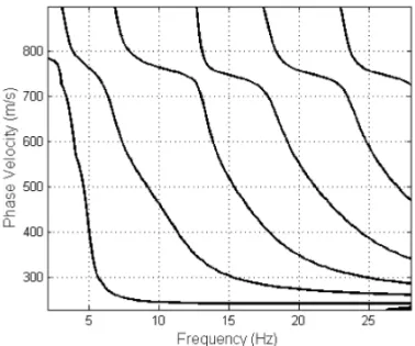
The dispersion curve (Fig. 1) relative to a model of heterogeneous layers can be generated through a nonlinear secular function
H(c, ω, ρ, α, β, d) = 0 (1) involving the physical parameters of density (ρ), P-wave veloc-ity (α), S-wave velocity (β), layer thickness (d), and phase ve-locity (c) (Thomson, 1950; Haskell,1953; Dunkin, 1965).
Figure 1 – Dispersion curves (modal nature).
The roots of the secular equation (Eq. 1) provide the phase velocities for each intended frequency valueω) and the param-etersρ, α, β, and d must be known during the modeling pro-cess. For each frequency value, one or more phase velocity val-ues are found, each integrating a different mode of the dispersion curve (Fig. 1). Studies often involve only the first mode (funda-mental mode) of the dispersion curve, but higher modes can be employed in the data modeling and inversion (Park et al., 1999b; Xia et al., 2003).
The theoretical dispersion curve is essential for the data inver-sion because it integrates the objective function, whose estimated minimum represents a good fit between theoretical and real data. In the data inversion, the objective function is used in an iterative procedure in which a set of initial values is required to start the inversion algorithm.
Deduction of the physical properties of a geological substrate through data measured by geophysical sensors is characterized by a process called the inverse problem. The goal of solving the inverse problem (data inversion) is to generate a model of the physical properties of the layers of interest as a function of depth.
For this, the field-acquired and subsequently processed data need to be adjusted to a theoretical model that associates these data with the depths investigated and the physical parameters of inter-est (S-wave velocity, density, resistivity, etc.).
The inverse problem can be solved by applying the least-squares method, as the Levenberg-Marquardt (Levenberg, 1944; Marquardt, 1963) procedure, which aims to minimize the residue between the experimental and theoretical data. For this, a good layers initial model to obtain a suitable data fit is required.
The layers initial model (depth as a function of S-wave veloc-ity) to the Rayleigh wave data inversion can be initially estimated scanning the real dispersion curve through equation
Z = P λ (2)
where, according to Abbiss (1981), the maximum penetration depth (Z) of a shear wave component is estimated to be between one-third and one-half (P ) of its wavelength (λ). In the study of the surface waves, the phase velocity (cn(λn)) must be converted
to an S-wave velocity (βn) during the scan of the dispersion curve:
βn =cn(λn)
Q (3)
whereQ is a conversion factor with a value between 0.87 and 0.96 (Richart et al., 1970).
The use of the Eqs. (5) and (6) allows estimating the S-wave velocities in predetermined layer thicknesses that will be used to start the data inversion algorithm. For more details, see Xia et al. (1999) and Lucena & Taioli (2014).
METHODOLOGY
The inversion program implemented in Matlab programming lan-guage uses the Levenberg-Marquardt algorithm to minimize the objective function and consequently fits the data between the real and inverted dispersion curves. In this process, parameters need to be calibrated and boundary conditions implemented to optimize the data inversion.
The P factor was calibrated as 0.5 (Lucena & Taioli, 2014). However, that value does not always lead to satisfactory data in-version and under these circumstances needs to be changed. In this work, the P factor is analyzed through its variation using as a reference the minimization of the values of the relative root mean-squared error (rRMSE) between the synthetic and inverted disper-sion curves calculated at the end of each data inverdisper-sion for more than 50 models. The rRMSE provides an indicator of inversion quality, where the lower its value, the better the data fit.
Two boundary conditions are implemented to improve data convergence. They can be applied in every interaction and their effectiveness was evaluated using the values of rRMSE gener-ated at the end of each data inversion. The first boundary con-dition ensures the S-wave velocities obey the minimum and max-imum limits of the phase velocities of the dispersion curve, us-ing Eq. (6) to convert the phase velocities to S-wave velocities. The second boundary condition ensures that the smallest Pois-son ratio is obeyed; in others words, the ratioαn/βnis never less than√2 during the data inversion.
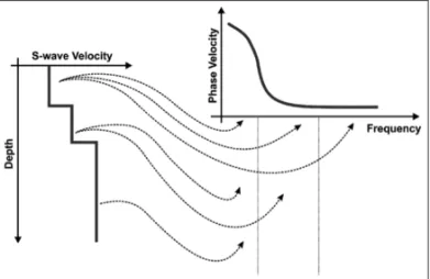
The post-inversion stage consists of a trial and error proce-dure started after the data inversion. Its goal is to create a fine fit between the real and inverted dispersion curves and conse-quently improve the inverted layered model. A fine fit is achieved by changing the S-wave velocities of the inverted layered model such that the inverted dispersion curve approximates the real dis-persion curve. Figure 2 provides a general idea of how each layer comprises a particular region of the dispersion curve and shows that the shallower layers help compose a larger region of the dis-persion curve, unlike the deeper layers that only help in the com-position of the low frequencies of the dispersion curve. Therefore, the procedure should be performed in the direction of low frequen-cies, starting with the shallower layers of the layered model.
Figure 2 – Scheme of the influence of each layer of a layered model in the
dis-persion curve (adapted from Strobbia, 2003).
Two tools were implemented in the post-inversion procedure to help the user choose better changes of the inverted layered model, resulting in a better data fit. With the first tool, the user indicates which point in the dispersion curve is to be changed and, in response, the tool indicates in which layer the velocity should be changed, using Eq. (5) for the estimation. The sec-ond tool generates a sensibility graph of the inverted model. This involves individually changing the S-wave velocity in 20% of each of the 10 layers of the inverted layered model and gen-erating a dispersion curve for each of the 10 changed layers.
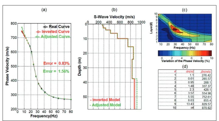
Figure 3 – Graphic interface of the post-inversion program.
The graph thus indicates the influence of each changed layer in the points of the dispersion curve, allowing the user to deter-mine which points in a particular frequency range will change with different intensities when a particular layer is modified. Fig-ure 3 shows the post-inversion program interface for the graphs of the dispersion curves (Fig. 3a), the layer model (Fig. 3b), the dependency of the dispersion curve with the variation of the S-wave velocities of each layer (Fig. 3c), and the table with the parameters αn, βn, and dn updated with every program adjustment (Fig. 3d).
In this initial interface, the user selects the point to be changed in the dispersion curve. Using an estimation of Eq. (5), the program suggests a layer to be changed, allowing the user to adjust the chosen point. The user can change the suggested layer or another layer, using as a reference the dependence of the dispersion curve along the 10 layers (Fig. 3c) and the table of layers model parameters (Fig. 3d). The fitted data are updated with every modification on the S-wave velocities until the end fit is achieved. Information relative to the last update is displayed in green so it can be compared to that of the previous update, displayed in red (Figs. 3a and 3b).
Using the post-inversion methodology accordingly and con-sidering the execution order and two tools described above, the procedure of trial and error can be well controlled by the user and is thus efficient.
This study was conducted on more than 50 models, with similar results to those presented here, characterized by the
re-sults for Models 1 to 3 reported in Table 1. The models have been used as input data to generate synthetic dispersion curves. The synthetic dispersion curves have been inverted and their in-verted models compared with the initial models (dnandβn of the Table 1).
Table 1 – Results for Models 1 to 3.
Models n (m/s)αn (m/s)βn (kg/mρn3) (m)dn αn/βn Model 1 1 170 100 1200 2 1.7 2 1020 600 2000 3 1.7 3 629 370 1900 7 1.7 4 1440 900 2100 ∞ 1.6 Model 2 1 1350 250 1900 4 5.4 2 2150 580 2200 5 3.7 3 2500 850 2500 ∞ 2.9 Model 3 1 600 280 1280 3 2.1 2 430 215 1200 5 2.0 3 1530 850 1950 ∞ 1.8
These models were chosen because they present different characteristics, such as contrasts of S-wave velocities between layers, with some models presenting velocity inversion and differ-ent Poisson ratios, as seen in the work of Lucena & Taioli (2014), that can significantly change the dispersion curves, interfering in the data inversion, and dispersion curves with different shapes, where the inversion algorithm will encounter difficulties in adjust-ing the data.
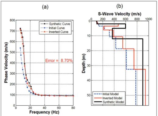
Figure 4 – Data inversion of Model 1, with a P factor equal to 0.5.
Figure 5 – Data inversion of Model 1, with a P factor equal to 0.3.
RESULTS AND DISCUSSION Setting the inversion parameters
The study of the 50 models shows, on average, that a P parameter equal to 0.5 is best to generate an initial model of layers close to the real layer model. However, this value does not always result in satisfactory data inversion. The inversion of Model 1 (Fig. 4), for example, shows that, despite the completion of five iterations and the good initial model generated, the fit between the inverted and synthetic dispersion curves has a high rRMSE.
Figure 4 shows good fit between the dispersion curves for the initial and synthetic models at high frequencies (above 30 Hz), but not at lower frequencies. When the P value is changed to less than 0.5, the dispersion curve for the initial model tends to move horizontally in the direction of higher frequencies. This can be seen in Figure 5, where the P parameter of Model 1 was changed to 0.3.
The initial model fit improves significantly at low frequencies with changes in the P parameter. Already at frequencies above 30 Hz, the fit becomes slight worse. This general improvement
in the fit between the initial and synthetic dispersion curves of Model 3 is reflected in the data inversion, whose errors decrease by approximately 8.7% to 4.6%.
Studying the other models shows that the high frequency re-gion of the synthetic dispersion curve is better represented by the initial model for high values of P, since the low frequency region is better represented for low values of P. Physically, this means that wave components with greater wavelengths lose effi-ciency at greater depths. Therefore, the method’s maximum depth of investigation does not reach 50% of the maximum wavelength and sometimes the maximum investigation depth approaches only 30% of the maximum wavelength.
During data processing, the user can generate an initial model with a P value equal to 0.5 and compare the initial dispersion curve generated with the real curve. The P value should be de-creased if the aim is to shift the initial dispersion curve toward high frequencies and increase the values of the phase velocity. If the aim is to shift the initial dispersion curve toward low fre-quencies and reduce the phase velocity, the P value should be increased. The computational cost to perform this task is low, be-cause at this stage the data inversion is not required. Figure 6 shows an example of adjusting P factor to generate the initial model relative to Model 2. The variation of this factor substan-tially interferes in the behavior of the dispersion curve of the ini-tial model and can be used as a tool to estimate the best iniini-tial dispersion curve to be used for the data inversion. In the case of Model 2, the yellow curve (P = 0.4) presents the best adjustment and is a good choice for the initial model to be inverted.
Figure 6 – Generation of initial dispersion curves for different P factor values
for Model 2.
Boundary conditions
The boundary conditions implemented in the inversion program correct unwanted results at each iteration. They can influence the
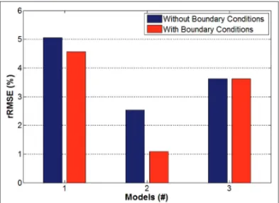
rRMSE, reducing it if a boundary condition is triggered during the data inversion. Figure 7 shows the interference in the rRMSE with and without the boundary conditions for Models 1 to 3.
Figure 7 – Influence of boundary conditions on the rRMSE for Models 1 to 3.
In all cases in which the boundary conditions are imple-mented, the rRMSE decreases or at least remains constant. We observe this behavior for the three models (Fig. 7) used to exem-plify the other 50 models: Models 1 and 2 show a significant drop in rRMSE values and, in Model 3, the boundary conditions don’t change the rRMSE value.
We found no cases where the rRMSE increases with im-plementation of the boundary conditions. This is because the boundary conditions correct for undesirable effects that occur at every iteration of the inversion process. When these corrections are necessary and are carried out, the inversion presents with an improved data fit; when there is no need for these corrections, the algorithm simply ignores the boundary conditions. Corrections are made when the minimum and maximum limits of the disper-sion curve are violated, given a margin of error of 30%.
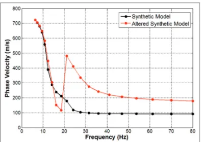
The boundary conditions should also be introduced to obey the minimum Poisson ratio (γ = 0 or αn/βn = √2). In a data inversion of the S-wave velocity totally independent of the previously set P-wave velocity values, the minimum Pois-son ratio cannot ever be obeyed and affect the data model-ing. Figure 8 illustrates this problem when the S-wave veloc-ity of the first layer of Model 1 that obeys the minimum Pois-son ratio (αn/βn = 1.7) is increased by 50% and the ratio αn/βndrops to about 1.13. The dispersion curve for the
mod-ified model is abruptly discontinued without any pattern and the dispersion curve is completely uncharacterized at approximately 14 Hz. The imposition of boundary conditions relative to the minimum Poisson ratio prevents errors in the initial modeling and in all iterations performed in the inversion process, avoiding
the inadequate convergence of data with the poor fit between the real and inverted dispersion curves.
Figure 8 – Dispersion curves relative to the original Model 1 (black line) and to
Model 1 with the S-wave velocity increased by 50% (red line).
Post-inversion program
The post-inversion trial and error program allows for the real-ization of a fine data inversion results fit. The main objective of improving the fit of regions where there is great discrepancy be-tween the points of the real and inverted dispersion curves that can significantly interfere in the model of generated layers. Fig-ure 3 shows the procedFig-ure implemented for Model 3, where the synthetic and inverted dispersion curves (Fig. 3a), the inverted layer model (Fig. 3b), the dependence of the dispersion curve as a function of the 10 inverted layers (Fig. 3c), and the table of the values of the number of layers, layer thicknesses, and the S-wave velocities of all the layers (Fig. 3d) are initially generated.
The graph of the dependence of the dispersion curve along the 10 layers (Fig. 3c) is extremely useful for showing the frequency regions in which and the intensity with which the dispersion curve is sensitized when the value of the S-wave velocity of a given layer is changed. It is important to perform this analysis for each model because the graphs of the dependencies are completely different for each model studied, as can be seen in Figure 9.
It is interesting to note that the shallower layers tend to sensitize the dispersion curve in a larger frequency range; in other words, when the S-wave velocity of the first layer is modi-fied, the high- and intermediate-frequency points of the disper-sion curve can be influenced and in some cases the low fre-quency points as well. The deepest layers concentrate their in-fluence at low frequencies (Fig. 9) and therefore do not affect the higher frequencies of the dispersion curve, as can be also seen in Figure 2. This information is important because it indicates that a fine fit should be achieved by initially modifying the
S-waves velocities of the shallow layers and then the velocities of the deeper layers.
Figure 9 – Dependence of the dispersion curve along the 10 layers for
(a) Model 1, (b) Model 2, and (c) Model 3.
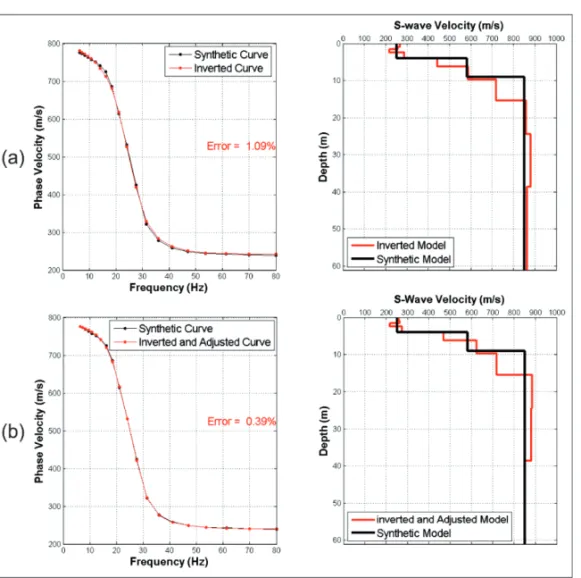
The trial and error procedure initiated in the first layers and finalized in the latest layers can be executed repeatedly, increas-ingly refining the adjustment between the dispersion curves. Figure 10 compares the inverted Model 2 (Fig. 10a) and its final fine fit (Fig. 10b).
For a simple layer model with a gradual increase in the S-wave velocity as a function of depth, as noted in Model 2 (Fig. 10), the improvement in the final fit of the data is slightly notice-able in the adjustment of the dispersion curves and of the layers model, with little interference in the final result, since in this sit-uation the data inversion is enough to generate a good data fit.
Figure 10 – Influence of the post-inversion data of Model 2: a) only the data inversion stage and b) the data inversion and post-inversion stages.
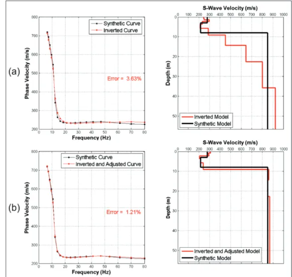
In more complex layer models with inversion of the velocities of the layers, for example, or abrupt changes in the dispersion curve, the inversion algorithm cannot obtain a good fit in these regions of abrupt changes or ripples generating adjustments with large values of rRMSE between the real and inverted dispersion curves. Thus, the post-inversion procedure significantly improves the ad-justment of the inverted data, highlighting S-wave velocity inver-sions and adjusting the inverted data to be closest to the real data. This situation is exemplified in Model 3, where the presence of a ripple is noted in the intermediate frequency of the dispersion curve due to the S-wave velocity inversion of the second layer. This inversion and fine adjustment can be seen in Figure 11, where the difference between the dispersion curve in the two procedures is quite pronounced.
Note that, as shown in Figure 11, the improvement in fit be-tween the dispersion curves, with the rRMSE falling from 3.63% to 1.21%, is positively reflected in the adjusted layer model, where the velocity inversion is very well defined.
The post-inversion procedure can replace the inversion pro-cess, that is, be its own data inversion in entirety. However, it is
advisable to perform the data inversion previously through an inversion algorithm, because the post-inversion procedure be-comes simpler and faster, since the process starts from a good data fit.
CONCLUSIONS
Each procedure adopted in this work improves, on average, the fit between the synthetic and estimated dispersion curves in the pre-inversion, pre-inversion, and post-inversion steps of the 50 studied models.
The study of the P parameter allows a greater understanding of the dispersion curve generated by the initial layered model. Thus the user can manipulate this parameter such that the esti-mated dispersion curve approximates the real dispersion curve, decreasing the mean-squared error in the pre-inversion stage.
In the inversion stage, the implemented boundary conditions help to accelerate data convergence and avoid anomalies caused in a free data inversion, where some iterations cannot obey the minimum Poisson ratio.
Figure 11 – Influence of the post-inversion data of Model 3: a) only the data inversion stage and b) the data inversion and post-inversion stages.
the refinement of the data, where the trial and error procedure di-rected through a priori information decreases the mean-squared error between the real and adjusted dispersion curves. This im-provement depends on the real data acquired, as well as the qual-ity of the data inversion. When the data show a dispersion curve with a smoothly varying S-wave velocity and data inversion with low mean-squared errors, the post-inversion stage improves the data fit very little and can even be omitted. However, when the real data acquired exhibit an abrupt change in velocities or ripples in their dispersion curve and the inversions present a high rRMSE, the post-inversion procedure significantly improves the data fit.
Therefore, the procedures described in this study and adopted together tend to improve the final result of the data inversion, especially in complex models with abrupt changes in veloc-ity or inversions in the S-wave velocities of the layers of the model studied.
ACKNOWLEDGEMENTS
The authors thank the Geosciences Institute of the Universi-dade de S˜ao Paulo for supporting the study of surface waves,
the Conselho Nacional de Desenvolvimento Cient´ıfico e Tec-nol´ogico (CNPq), the CAPES-PROAP-RMH-2013 by the finan-cial support and Dr. Claudio Strobbia for his help in one of the modeling stages of the Rayleigh waves in our work.
REFERENCES
ABBISS CP. 1981. Shear wave measurements of the elasticity of the ground. Geotechnique, 31(1): 91–104.
BANIASADI E, RIAHI MA & CHAYCHIZADEH S. 2009. Determination of 1-D shear-wave velocity profileusing the refraction microtremor method. In: Shiraz 2009-1st EAGE International Petroleum Conference and Exhibition.
DUNKIN JW. 1965. Computation of modal solutions in layered, elas-tic media at high frequencies. Bulletin of the Seismological Society of America, 12: 335–358.
FOTI S. 2000. Multistation methods for geotechnical characterization us-ing surface waves. Doctoral dissertation, Politecnico di Torino. 230 pp. HASKELL NA. 1953. The dispersion of surface waves on multilayered media. Bulletin of the Seismological Society of America, 43: 17–34.
HORIKE M. 1985. Inversion of phase velocity of long-period micro-tremors to the S-wave velocity structure down to the basement in urban-ized areas. Journal of Physics of the Earth, 33: 59–96.
LEVENBERG K. 1944. A method for the solution of certain nonlin-ear problems in least squares. Quarterly of Applied Mathematics, 2: 164–168.
LOUIE JN. 2001. Faster, better: shear-wave velocity to 100 meters depth from refraction microtremor arrays. Bulletin of the Seismological Society of America, 91(2): 347–364.
LUCENA RF & TAIOLI F. 2014. Rayleigh wave modeling: A study of dis-persion curve sensitivity and methodology for calculating an initial model to be included in an inversion algorithm. Journal of Applied Geophysics, 108: 140–151.
MARQUARDT DW. 1963. An algorithm for least-squares estimation of nonlinear parameters. SIAM Journal on Applied Mathematics, 11(2): 431–441.
NAZARIAN S & STOKOE KH. 1984. In situ shear wave velocities from spectral analysis of surface waves. In: Proceedings of the World Confer-ence on Earthquake Engineering, Vol. 8, San Francisco, CA, pp. 21–28. PARK CB, MILLER RD & XIA J. 1999a. Multichannel analysis of surface waves. Geophysics, 64: 800–808.
PARK CB, MILLER RD, XIA J, HUNTER JA & HARRIS JB. 1999b. Higher mode observation by the MASW method. In: Exp. Abstracts of the Tech-nical Program with Biographies, Society of Exploration Geophysicists,
69th Annual Meeting, Houston, TX, Society of Exploration Geophysi-cists, Tulsa, OK, pp. 524–527.
PARK CB, MILLER RD, RYD´EN N, XIA J & IVANOV J. 2005. Combined use of active and passive surface waves. Journal of Environmental & Engineering Geophysics, 10(3): 323–334.
RICHART Jr FE, HALL JR & WOODS RD. 1970. Vibrations of Soils and Foundations. Prentice Hall, NJ. 437 pp.
RYDEN N & PARK CB. 2006. Fast simulated annealing inversion of surface waves on pavement using phase-velocity spectra. Geophysics, 71: R49–R58.
STROBBIA C. 2003. Surface wave method acquisition, processing and inversion. Ph.D. Thesis, Polytechnic University of Turin. 317 pp. THOMSON WT. 1950. Transmission of elastic waves through a stratified solid medium. Journal of Applied Physics, 21: 89–93.
WATHELET M, JONGMANS D & OHRNBERGER M. 2004. Surface wave inversion using a direct search algorithm and its application to ambient vibrations measurements. Near Surface Geophysics, 2: 211–221. XIA J, MILLER RD & PARK CB. 1999. Estimation of near-surface shear-wave velocity by inversion of Rayleigh shear-waves. Geophysics, 64: 691–700. XIA J, MILLER RD, PARK CB & TIAN G. 2003. Inversion of high fre-quency surface waves with fundamental and higher modes. Journal of Applied Geophysics, 52: 45–57.
Recebido em 21 marc¸o, 2016 / Aceito em 14 junho, 2017 Received on March 21, 2016 / Accepted on June 14, 2017