Modes of infrastructure financing and the ‘Big Push’ in development economics

Joana Pais, José Pedro Pontes

Modes of infrastructure financing

and the ‘Big Push’ in development

economics

WP01/2016/DE

_________________________________________________________

WORKING PAPERS

Modes of infrastructure financing

and the ‘Big Push’ in development

economics

Joana Pais1 _{and José Pedro Pontes}2

4/01/2016

Abstract: In an economy where different agents undertake simultaneous and interdependent investments, this paper models the possibility that the outcome where some players invest and others do not invest is sustained in Nash equilibrium. It is well known that in models where all goods are financed through prices charged by the suppliers (“tolls” in the case of transport infrastructures), there are only two coordination equilibria: the “Big push” equilibrium, where every agent involved invests; and the “Poverty trap”, whenever none invests. We consider a two person simultaneous game, where the Government decides whether to build a highway and a firm producing a composite good decides whether to use it. Instead of resorting to tolls, the infrastructure is funded through an income tax that falls on wages. Having the Government supplying the highway and the firm not using it is a Nash equilibrium if the employment generated by the construction of the highway is intermediate and the rate of the wage income tax is high. The proliferation of unused transport infrastructures in Southern Europe seems to be related with low effects of public works upon the demand for labor and with demand-depressing “austerity” macroeconomic policies.

JEL Classification: C72, 011, R11.

Keywords: Balanced growth, Big Push, Spatial Concentration, Infrastructures Policy, non-cooperative games.

1.

Introduction

Economic development is widely regarded as following from a set of complementary investment decisions by independent agents, namely private firms and the Government. In this setting, the state is supposed to build infrastructures that improve the connection between production and consumption, for instance, transport networks. Firms are assumed to switch from a production regime based upon many small plants, which work under constant returns and sell only to nearby consumers to a production structure with a small number of large plants, working under increasing returns and exporting the product over long distances.

We may name the first production regime as achieving “proximity” to consumers, while the second one is usually regarded as a productive structure based upon “spatial concentration”. In the economic geography literature, productive concentration is usually associated with a rise in labor productivity on account of different causes:

• Increased division of labor, allowing workers to specialize in different simple tasks, which are performed more efficiently (STIGLER, 1951).

• Increased output at the plant level allows the use of fixed inputs, such as machinery, which increase labor productivity (MURPHY et al., 1989).

• In economies where growth follows from the creation of new products, the rate of innovation is higher in regions where relatively more products have been invented and produced previously (see MARTIN and OTTAVIANO, 1999).

Complementarities between separate investments arise both at the “demand” and at the “cost” levels. At the demand level, geographical concentration of production and the increase of its output raise the potential demand for transport services, thus enabling a transport infrastructure, e.g., a highway to break even. At the cost level, a transport infrastructure decreases transport costs for goods and allows the firms to export over long distances. Consequently, they no longer have to be in the proximity of their customers and may therefore to concentrate production in larger, more productive plants.

It is possible to model the process of economic development in two different ways. According to the first way, following HIRSCHMAN (1958), development is regarded as a pure sequential game, a sequence of investments causing imbalances that are progressively corrected and temporarily offset by foreign trade flows. The problem of this approach is that it leads to a unique and efficient equilibrium, free from the failures that are usually met in real-world situations.

However, the “Big Push” model does not account for the recent experience of Southern European countries, where highways have been built at a high pace by national governments with the aid of European Funds (Structural Funds and European Funds). For instance, in Portugal, highways grew in length at an average annual rate of 5.8% between 2000 and 2012 (see also TEIXEIRA, 2006). Nevertheless, most firms continued to adopt strategies of proximity to consumers rather than geographic concentration, since:

• Labor productivity did not rise significantly: real per capita GDP and nominal industrial wage practically stagnated during this period.

• There was a reallocation of resources. Non-tradable goods (mainly services) substituted for tradable goods (for instance, industrial goods). The former must be supplied in the local where they are consumed, whereas the latter can be exported.

• There was a reallocation of resources away from increasing returns sectors (such as manufacturing) towards constant returns resource based sectors (such as agriculture and tourism).

• Many highways always had a very low rate of use, so that they can be labeled as “white elephants.” This fact concerns particularly those that cross regions with low demographic and productive density.

This trend was magnified by the recent recession. According to the operator Brisa, the traffic on highways with tolls fell 15.3% in the first semester of 2012 relative to the same period in the previous year. In the first semester of 2013, the use of highways with tolls fell again 6.3% relative to the same period of 2012.

The evolution of other Southern European countries is similar to the Portuguese experience: governments have built the infrastructures but productive units often failed to switch to concentrated patterns and to increase labor productivity. Consequently, the new highways remained unused in large measure. This outcome is not previewed in the “Big Push” model, where either all agents invest, or none does. We need to modify this model in order to account for the possibility of a “white elephant” highway or airport to emerge.

In this paper, we find that the key factor is the financing mode of the public infrastructure, where the “Big Push” is related with a financing made by tolls paid by the users, whereas the asymmetric outcome concerns infrastructures paid for by income taxes.3 _{In what follows, the}

two models for financing public infrastructures are dealt with and related with different economic development situations.

The structure of the paper is as follows. We present the assumptions of the model in section 2. In section 3, the “Big push” outcome is seen to emerge from the financing the infrastructure construction by means of tolls. The likelihood of building an infrastructure without causing industrial development (the so called “white elephant” outcome) is related to financing public works through wage income taxes in section 4. Section 5 gathers the main conclusions.

3 _{In this case, public infrastructures will be paid for by taxes falling on wages, either immediately or}

2.

The model

Our spatial economy complies with the following assumptions:

1. The economy is made up by two symmetric regions: A and B. The set of consumers/workers in each region is expressed by a representative consumer.

2. The economy entails the production of a composite consumer good by a sector of firms and the building of a transport infrastructure (a highway, w.l.o.g.) by the Government. Labor is the only factor of production.

3. The utility of the composite good for each representative consumer is positive and strictly increasing in consumption. In particular, the consumers’ demand for this good is

given by

q

y

p

=

, where

y

is the consumer’s income. Each representative consumer

supplies

L

₀ units of labor in the absence of a transport infrastructure and

L

>

L

₀ units of labor otherwise. The difference between

L

and

L

₀ accounts for the expansionary effect of infrastructural investment on the demand for labor.

4. The composite consumer good is produced by a fringe of competitive firms that operate under constant returns and sell only to consumers living in the same region. In spatial terms, each one of these firms chooses a strategy of “proximity to consumers”. Among these firms one has the option to become a monopolist, switching to an increasing returns technology. This firm can sell locally and furthermore it can export the output to the other region. In spatial terms, it chooses a “geographic concentration” strategy for its productive activity.

5. The wage in the consumer good industry is equal to 1 m.u. for all possible outcomes, with the exception of the particular case when both the private firm and the Government perform investments. In this eventuality, the firm can pay wage w, with

1

w> , since labor productivity increases now to

α

>1. Moreover, it must pay w

because the firm now employs foreign workers who incur commuting costs of w−1

across the two regions.

6. The technology used under “consumer proximity” is constant returns: one unit of labor is transformed into one unit of consumer good, without the aid of any fixed inputs. Hence, the price of the consumer good is 1 m.u. and profits are zero. The “geographic concentration” technology is increasing returns: one unit of labor is transformed into

1

α

> units of consumer good, using in addition a fixed input (a machine), that costs

F

units of labor valued at the current wage rate. It is assumed that the supply of labor by a representative consumer covers the construction cost of the fixed asset, so that

0

L

>

F

holds.

competitive fringe of firms. On the other hand, since the price elasticity of demand is 1, it would not gain by decreasing the price below 1.

8. It is assumed that

α

>w, so that the unit operative profit of the “concentrated”

technology 1 w

α

 

−

 

 is positive, where

w

α

represents the unit labor cost under this

regime.

9. If the highway is built, transport cost of the composite good across regions A and B is

0

ε

> , arbitrarily small. Otherwise, the transport cost is m 1 w

α

 

>_ − _

 , so that

transporting the consumer good across the regions is prohibitive.

10. The construction of the highway amounts to

R

units of labor, valued at the current wage. It is assumed that the total labor supply by the two representative consumers

2

L

covers the construction cost of the fixed assets used in producing and moving goods, so that condition

2

L

>

F

+

R

is always met.

3.

Financing the highway through a toll: the “Big Push”

economy

The economy can be modelled through a

2 2

×

non-symmetric game, whose payoff matrix is

11 11 12 12

21 21 22 22

Firm

Concentration

Proximity

Government

Build Highway

,

,

Not build

,

,

a

b

a

b

a

b

a

b

(3.1)

Since the construction cost of the highway is Rw, the Government charges a toll to the “geographically concentrated” plant that uses the highway to export its output to the other region. This toll has the amount

Rw

+

δ

, with

δ

positive and arbitrarily small. The Government’s payoff is the difference between the toll – whenever it is charged – and the construction cost of the infrastructure. Hence, its payoffs are:

(

)

11

0, arbitrarily small

a

=

Rw

+

δ

−

Rw

=

δ

>

(3.2)

21

0

a

=

(3.3)

12

0

0

22

0

a

=

(3.5)

We now determine the firm’s payoffs. These are zero if the firm adopts a “proximity” locational strategy, so that we have

12 22

0

b

=

b

=

(3.6)

Inserting (3.2) to (3.6) into (3.1), we obtain the simplified payoff matrix that follows:

11

21

Firm

Concentration

Proximity

Government

Build Highway

,

, 0

Not build

0,

0, 0

b

Rw

b

δ

−

(3.7)

It is clear that the game shown in matrix (3.7) is a coordination game with two strict Nah equilibria (Build, Concentration) and (Not Build, Proximity) if and only if the following two conditions are met:

11

0 and

b

>

(3.8)

21

0

b

<

(3.9)

We now try to assess the meaning of conditions (3.8) and (3.9).

Since

b

₁₁ is the profit of a concentrated firm that supplies both the domestic market and the host market through exports, incurring in a toll for that purpose, we have:

(

)

11 1 1

w w

b

π

ε

y y Fw Rw

δ

α

α

   

= =_ − − _ +_ − _ − − +

    (3.10)

Consequently, we have:

(

)

11 2 1

w

b

π

y F R w

α

 

= ≈ _ − _ − +

  (3.11)

On the other hand, as we are considering the case in which the highway is built, each representative consumer sells an amount

L

of labor to composite good production and to infrastructure construction. Hence, her income is given by:

2

y

=

π

+

wL

(3.12)

(

)

11 2 1

w

b

π

L F R

α

 

= = _ − _− +

  (3.13)

We now determine

π

≡

b

₂₁. As the transport cost without the infrastructure is prohibitive

i.e., m 1 w

α

 

> −

 

 , the “concentrated” firm sells only in its domestic market. The other region is

supplied by competitive firms that follow the strategy of “proximity to consumers”. Profit by the “spatially concentrated” firm is then given by:

21

1 1

b

π

y F

α

 

= =_ − _ −

  (3.14)

The representative consumer’s income becomes:

0

2

y

=

π

+

L

(3.15)

In (3.15),

L

₀

<

L

is the amount of labor exclusively dedicated to the production of the consumer good. Substituting (3.15) in (3.14) and solving, the firm’s profit

b

₂₁ becomes

(

)

21 0

2

1

1

b

π

L

α

α

F

α

=

=



_

−

−



_

+

(3.16)

Considering together inequalities

b

₁₁

>

0 and

b

₁₂

<

0

, we observe that only variables

α

and F

that are common to both of them. Hence, we will treat these inequalities as functions

α

( )

F

. According to (3.13), inequality

b

₁₁

>

0

is equivalent to:

(

)

( )

2

2

Lw

F

L

F

R

α

>

=

α

−

+

(3.17)

Given assumption 10 in section 2, function

α

( )

F

is continuous and positively valued in the domain

[

0,

L

₀

)

. Its main properties are:

1.

α

( )

0

>

1

.

2.

α

( )

F

is strictly increasing.

3.

α

( )

F

is strictly convex.

4.

( )

₀

0

2

tends to finite and positive, when 2

Lw

F F L

L L R

α

→

According to (3.16), inequality

b

₂₁

<

0

is equivalent to:

( )

0

0

L

F L F

α

< =

α

− (3.18)

The function

α

( )

F

is positively valued and continuous in the domain

[

0,

L

₀

)

. In addition, it has the following properties:

1.

α

( )

0

=

1

.

2.

α

( )

F

is strictly increasing.

3.

α

( )

F

is strictly convex.

4.

( )

0

lim

F→L

α

F = +∞.

Using (3.17) and (3.18), we define the function

α

( )

F

in the domain

[

0,

L

₀

)

as follows:

( )

F

( )

F

( )

F

α

≡

α

−

α

(3.19)

It is clear that:

( )

0

( )

0

( )

0

2

1 0

2 wL L R

α

≡

α

−

α

=

= − <

−

(3.20)

In addition, we have:

( )

( )

( )

0 0 0

0

lim lim lim

2 2

F L F F L F F L F

wL L L R

α

α

α

→ = → − → =

= +∞ − = +∞

− −

(3.21)

Since the fraction in the r.h.s. of (3.21) is finite,

α

( )

F

tends to infinity whenever the productive

fixed cost

F

approaches L₀. Given that (3.20) and (3.21) hold and function

α

( )

F

is a

continuous function, there is a level of the fixed cost in production, L, such that

α

( )

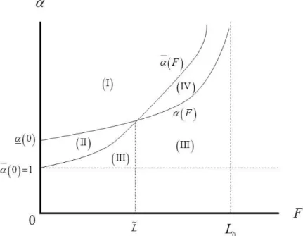
L =0. Let

In Figure 1, the following regions of Nash equilibria are plotted:

• Region (I), where b₁₁>0 and b₂₁ >0: a unique Nash equilibrium (Build, Concentration).

• Region (II), where b₁₁<0 and b₂₁>0: no Nash equilibrium in pure strategies.

• Region (III), where b₁₁<0 and b₂₁<0: a unique equilibrium (Not Build, Proximity).

• Region (IV): where b₁₁ >0 and b₂₁<0: there are two equilibria: (Build, Concentration) and (Not Build, Proximity).

Hence, the investment game becomes a coordination situation if the productive fixed costs are high and the jump in labor productivity following firm concentration is intermediate.

4.

Economic development when the infrastructure is financed by

means of an income tax

Instead of being paid for by those firms who actually use the infrastructure through tolls, we now assume that the highway is financed directly by the Government. An income tax with a rate

t

∈

(

0,1

)

, which falls on wages, is used to support the construction cost of the highway.

We reproduce here matrix (3.1).

11 11 12 12

21 21 22 22

Firm

Concentration Proximity

Government Build Highway , ,

Not build , ,

a b a b

a b a b

The Government payoffs, a_ij, i j, =1, 2, correspond to the budget surplus, i.e. the difference between the fiscal revenue, T_ij, and the highway construction cost, calculated using the wage rate prevailing in the composite good industry. Hence, we can write the government’s payoffs as:

(

)

(

)

11 11

2

2

a

=

T

−

Rw

=

Lwt

−

Rw

=

w

Lt

−

R

(4.1)

(

)

12 12

2

2

a

=

T

−

R

=

Lt

−

R

=

Lt

−

R

(4.2)

21 21 0 0 2 0

a =T =L t+L t= L t (4.3)

22 22 2 0

a =T = L t (4.4)

In turn, we evaluate the composite good firm’s payoffs. It is known that, if the firm chooses the “proximity to consumer “ strategy, its payoffs are zero, as the firms work under perfect competition and use a constant returns technology. Consequently, we have

12 22 0

b =b = (4.5)

In contrast, the firm’s payoff when it adopts a “spatially concentrated” strategy and the Government builds the highway is

(

)

11 1 1 1 2

w w w

b y y Fw y Fw

π

ε

α

α

α

     

= =_ − − _ +_ − _ − ≈_ − _ −

      (4.6)

(

1

)

2

y

=

π

+

wL

−

t

(4.7)

Inserting (4.7) into (4.6) and solving, we obtain:

(

)(

)

11

2

1

b

L

t

w

F

π

=

=

−

α

−

−

α

(4.8)

The firm’s profit when it concentrates the production in space but is unable to export because the highway is not built by the Government is:

21

1 1

b y F

π

α

 

= =_ − _ −

  (4.9)

The representative consumer’s income is

(

)

0

1

2

y

=

π

+

L

−

t

(4.10)

Plugging (4.10) into (4.9) and solving, we get

(

)(

)

21 0

2

1 1

1

b

L

t

F

π

α

α

α

=

=



_

−

−

−



_

+

(4.11)

(

)

(

)(

)

(

)(

)

0 0 0

Firm

Concentration Proximity

Government Build Highway 2 , 2 1 2 , 0

2

Not build 2 , 1 1 2 , 0

1

w Lt R L t w F Lt R

L t L t F L t

α

α

α

α

α

− − − − −

− − −

 

 

+

(4.12)

It is easy to simplify matrix (4.12) to one containing zero outside the main diagonal. For that purpose, the off-diagonal payoff in each row (for player Government) and each column (for player Firm) is subtracted to the elements of that row or column. This transformation merely displaces locally the payoff function of each player, keeping intact the best reply structure, the dominance relationships between the strategies and the set of Nash equilibria of the game. It yields the following diagonal matrix:

(

)

(

)(

)

(

)

(

)(

)

1 0 1

2 0 2 0

Firm

Concentration

Proximity

Government

Build Highway

2

,

2

1

0, 0

2

Not build

0, 0

2

,

1 1

1

a

t Lw L

Rw b

L

t

w

F

a

R

t L

L

b

F

L

t

α

α

α

α

α

=

−

−

=

−

−

−

=

−

−

=



_

−

−

−



_

+

The payoff matrix (4.13) defines a class of games. We will consider the subset of this class where the outcome (Build, Proximity) is a strict Nash equilibrium. This subclass is defined (if we refer to matrix (4.13)) by inequalities:

2<0 and 1 0

a b < i.e.

(

0

)

2

<0

R

−

t L

−

L

(4.14)

(

)(

)

2

L

1

−

t

α

−

w

−

α

F

<

0

(4.15)

The two parameters that are common to both inequalities, (4.14) and (4.15), are

(

the income tax rate

)

t

≡

and

L

(

≡

the maximum amount of labor available in each region

)

.

By solving (4.14) and (4.15) in order to t, we can define bounds on this parameter for each possible value of

L

. The bound t Lɵ

( )

can be obtained by solving (4.14) in order to

L

in order to obtain:

(

0

)

( )

2

R

t

t L

L

L

>

=

−

ɵ

_(4.16)

In addition, the bound t Lɶ

( )

can be found by solving (4.15) in order to t so as to get:

(

)

( )

1

2

F

t

t L

L

w

α

α

> −

=

−

ɶ

(4.17)

We seek now to find the properties exhibited by the boundary functions in (4.16) and (4.17).

4.1

Properties of

t Lɵ

( )

• The function t Lɵ

( )

is defined in the domain

(

L

₀

,

+∞

)

.

• It is strictly decreasing.

• It is strictly convex.

• t Lɵ

( )

tends to + ∞ when L→L₀. Hence, the lower bound of

t L

( )

is given by

( )

{

}

min t Lɵ ,1 .

• lim

( )

0

L→+∞t L =

4.2

Properties of

t Lɶ

( )

• The function t Lɶ

( )

is defined in the domain

(

L

₀

,

+∞

)

• It is strictly increasing.

• It is strictly concave.

•

( )

(

)

0

0

0

lim 1

2

L L

F t L

L w

α

α

→

 

= − 

−

 

ɶ . Since, by assumption,

α

>w holds, the fraction

within brackets is positive. Consequently,

( )

0

0

lim

L→L t L

ɶ _{is not higher than 1.}

Nevertheless, this limit can be negative. Hence, we write the lower bound function of

( )

t L

as max 0,

{

t Lɶ

( )

}

.

• lim

( )

1

L→ +∞t L =

ɶ .

From Figure 2, one can infer that the “white elephant" equilibrium, i.e., the equilibrium (Build, Proximity) arises as a strict Nash equilibrium depending on two conditions:

1. The increase in employment following from the construction of the transport infrastructure,

(

L

−

L

0

)

, should be intermediate, neither too low nor too high. In fact, on the one hand, if

(

L

−

L

0

)

is small, the increase in taxes on wages determined by the construction of the

hand, if the rise in the wage income caused by the public works is too high, the jump in market demand for the composite consumer good leads the producers to switch from a spatially dispersed technology to a geographically concentrated one.

2. The tax rate on wages should be high enough in order to ensure that a strong rise in employment and wage income, brought about by the public works, does not lead to a meaningful rise in market demand for the composite good, which would determine a technological switch and a productive locational concentration.

However, instead of a pure strategy strict Nash equilibrium, the outcome (Build, Proximity) may be associated to a mixed strategy equilibrium, where the equilibrium strategy by the Firm is completely mixed, but the Government still builds the highway with probability one. Let

(

0,1

)

p

∈

be the probability with which the Firm chooses “Proximity.” Then, the range of

p

can determined by the following inequality (see payoff matrix (4.13)):

(

1−p

)

2t Lw

(

−L0

)

−Rw> p R −2t L

(

−L0

)

 (4.18)

The solution of (4.18) is:

(

)

(

)(

)

0

2

1 2

t Lw L Rw p

w tL R

− −

<

− − (4.19)

The assumptions ensure that the denominator of the r.h.s. of (4.19) is positive. In particular, we have2tL>R, since the tax revenues must cover the fixed cost of highway building.

Moreover, we must check that (4.19) is compatible with the constraints on

p

, i.e. p>0. Using (4.19), it is easy to conclude that:

(

0

)

( )

0

2

Rw

p

t

t L

Lw L

> ← >

≡

−

(4.20)

The inequality in (4.20) defines a lower bound function

t L

( )

for the tax rate for each value of

L

. The properties of the lower bound function

t L

( )

are:

• The domain is 0

, L w   +∞  

  since

0

0

0

L

Lw L

L

w

−

> ↔

>

.

•

t L

( )

tends to +∞ when

L

0

L

w

→

.

•

lim

( )

0

L→+∞

t L

=

•

t L

( )

is strictly decreasing.

In addition, in order that a completely mixed strategy 0< p<1 is a best reply by the Firm to the choice of “Build Highway” by the Government the payoffs of its pure strategies “Concentration” and “Proximity” should be equalized.

This amounts to say that, in payoff matrix (4.13), the following condition should be met:

(

)(

)

1

2

1

0

b

=

L

−

t

α

−

w

−

α

F

=

(4.21)

By solving (4.21) for t, we get the following value for the tax rate:

( )

(

)

1

2

F

t L

L

w

α

α

= −

−

(4.22)

The properties of

t L

( )

in (4.22) are:

• The domain is

(

L

₀

,

+∞

)

.

• The sign of

( )

0

lim

L→L t L is indeterminate. This follows from both assumptions, 0 and

F <L

α

>w.

•

lim

( )

1

L→+∞

t L

=

.

•

t L

( )

is strictly increasing.

•

t L

( )

is strictly concave.

We note that mixed equilibria emerge if the employment effect of the investment in a highway is large and it is partially offset by an increase of the income tax falling on wages.

The mixed strategy equilibrium allows us to model the effect of incomplete information by the Government concerning the profits earned by the Firm under its two strategies, namely “Concentration” and “Proximity”. If the Government is aware that the difference in profits is relatively small and partially unknown, then the public authority can model the Firm’s behavior as if conformed to a mixed strategy.

5 Conclusions

Given the results in this paper, we can conclude that a model of economic development based on simultaneous and interdependent investments by different agents can account for an outcome where the Government builds a transport infrastructure but the firms fail to switch to a more geographically concentrated technology which would enable them to use the highway. Instead the firms remain stuck in small scale, proximate to consumer technologies, so that the highway remains largely unused and becomes a “white elephant.”

This kind of equilibrium arises only if the public investment is paid for by wage income taxes rather than through tolls contributed by the highway users. This outcome is more likely to happen if employment creation promoted by the infrastructural investment is either very low or very high and the tax rate is high. If the employment creation by the public works is very low, its impact upon consumers’ income and fiscal revenues is also small. Under these circumstances, the Government decides not to undertake the construction of the highway.

By contrast, if building the transport infrastructure expands the employment very much, then,

ceteris paribus, the aggregate wage income rises, causing a steep increase in market demand for consumer goods. Faced with this market demand increase, the firms producing consumer goods have a strong incentive to shift to technologies that are more intensive in fixed inputs and also more geographically concentrated. All in all, the highway is supplied and it is used by the firms.

In any case, a high wage tax rate curtails the consumers’ disposable income and the aggregate market demand, thus preventing the firms to switch from constant returns technology, where the firms sell mainly to local consumers, to an increasing returns productive system where the firms export over long distances. High taxes are thus correlated with highway idleness.

Consequently, fiscal tightness in Southern European countries, such as Portugal, is likely the main cause behind the resource waste embedded in idle highways and airports that were built and then became almost unused.

In this paper, we dealt with economic development dilemmas by means of defining a causal relation between the modes of financing infrastructures by the Government and the set of Nash equilibria in the investments coordination game.

An alternative research line, which we intend to follow in the future, is to associate economic development with the selection of a unique equilibrium in the game of investment coordination. For that purpose, we could resort to several different methodologies.

for the sender and does not bind his behavior in any sense, so that it is called “cheap talk” (FARRELL and RABIN, 1996).

The second approach to select a unique equilibrium in the coordination investments game would deductive as it would use only the mathematical structure of the game (HARSANYI and SELTEN, 1988). In this case, the players would select the equilibrium that is supported for each player by the widest range of probabilistic beliefs concerning the intentions of the his

6 References

COOPER, Russell W. (1999), Coordination Games – Complementarities and Macroeconomics, Cambridge, Cambridge University Press.

FARRELL, Joseph and Mathew RABIN (1996), “Cheap Talk”, Journal of economic Perspectives,

10(3), pp. 103-118.

HARSANYI, John C. and Reinhardt SELTEN (1988), A General Theory of Equilibrium Selection in Games, London and Cambridge/Mass., MIT Press.

HIRSCHMAN, Albert O. (1958), The Strategy of Economic Development, New Haven (USA), Yale University Press.

LEWIS, David (2008), Convention: A Philosophical Study, John Wiley and Sons.

MARTIN, Phillipe and Gianmarco I.P. OTTAVIANO (1999), “Growing locations: Industry location in a model of endogenous growth,” European Economic Review, 43, pp. 281-302.

MURPHY, Kevin M., Andrei SHLEIFER and Rober W. VISHNY (1989), “Industrialization and the Big Push”, Journal of Political Economy, 97(5), October, pp. 1003-1026.

ROSENSTEIN - RODAN, P. N. (1943), “Problems of industrialisation of Eastern and South-Eastern Europe”, Economic Journal, 53(210/211), September, pp. 202-211.

STIGLER, George (1951), “The division of labor is limited by the extent of the market”, Journal of Political Economy, 59, pp.185-193.

TEIXEIRA, A. C. Fernandes (2006), “Transport policies in the light of the new economic