Efficiency in school education: a semi-parametric study of shool efficiency in OECD countries

(1)

A semi-parametric study of school efficiency in OECD countries

Gonçalo da Silva Lima

Dissertation submitted as partial requirement for the conferral of

Master in Economics

Supervisor:

Prof. Henrique Monteiro, Prof. Auxiliar, ISCTE Business School,

Departamento de Economia

(2)

(3)

To my late grandpa A..

To my mum, my moral compass.

To my sister, who always put up with me, against all odds. To my dad, who – even from afar – was always present.

To all my family and friends, that nurtured me and shaped me to be who I am today. To Paris, that keeps inspiring me.

Gratitude to all work and university colleagues from whom I have learned immensely. Special mention to my team, that allowed me to grow professionally and as a person.

To my supervisor, that always supported me through the most stressful moments of this dissertation.

And last, but not the least: to Emma. Thank you for all your encouragement and help!

(4)

Efficiency-driven reforms have become increasingly relevant in education policy, as edu-cation systems face tighter budget constraints. Eduedu-cational authorities around the world often struggle to foster the best student outcomes out of the set of available school re-sources. This dissertation aims to contribute to this debate by using a semi-parametric approach to evaluate the efficiency across 34 OECD countries, using data from PISA 2015. The estimation of the education production possibilities frontier is made through a free disposal hull (FDH) method, a non-convex and non-parametric estimator, also extend-ing the analysis to incorporate recently developed partial frontier methods (order-m and order-𝛼). According to the different specifications, inefficient schools could have increased average student achievement between 9%-18%, for the same level of human and material resources, and given the socio-economic characteristics of their students. Differences in efficiency scores are also investigated. The results suggest that schools that enrol a larger number of students and where the principal can decide on budget allocations are more efficient. On the other hand, schools with high concentration of students from immigrant backgrounds and more repeaters are hindered in the provision of efficient allocations of school resources. Finally, no necessary trade-off is found between efficiency and equity in the provision of quality education.

Keywords: School efficiency, OECD, free disposal hull (FDH) estimator, partial fron-tiers analysis.

(5)

Reformas tendo em vista aumentos de eficiência têm-se tornado crescentemente relevantes na definição de políticas educativas, especialmente no contexto de orçamentos educativos mais limitados. Neste sentido, responsáveis em diferentes sistemas educativos têm ten-tado saber como melhorar os resulten-tados dos alunos, dados os recursos escolares disponíveis. Esta dissertação tem por objectivo contribuir para este debate, através de uma avaliação semi-paramétrica de eficiência escolar em 34 países da OCDE, recorrendo a dados do PISA 2015. Estimamos a fronteira de possibilidades de produção educativa através de

free disposal hull (FDH), um estimador não-paramétrico e não-convexo. Também

esten-demos a análise para incorporar métodos de fronteiras parciais (order-m e order-𝛼). De acordo com as diferentes especificações, as escolas ineficientes na amostra poderiam ter aumentado a qualidade de educação entre 9% e 18%, utilizando o mesmo nível de rescur-sos humanos e materiais, e tendo em conta as características socio-económicas dos seus alunos. A variação nos scores de eficiência é também investigada. Os resultados sugerem que escolas com um maior número de alunos e em que o diretor tem poder de decisão sobre a alocação do orçamento escolar são mais eficientes. Por outro lado, escolas com maior concentração de alunos de contextos familiares de imigração e com mais repetentes têm maior dificuldade em se aproximar da fronteira internacional de eficiência. Por fim, não há evidência de um trade-off necessário entre eficiência e equidade na provisão de educação de qualidade.

Palavas-chave: Eficiência escolar, OCDE, free disposal hull (FDH), análise de fronteiras parciais.

(6)

List of Figures

4.1 FDH and DEA frontiers . . . 21 4.2 Metafrontier illustation . . . 25

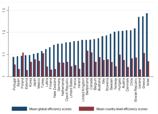
6.1 Mean global and country-level efficiency scores by country (raw efficiency) 39 6.2 Mean global and country-level efficiency scores by country (after

account-ing for ESCS) . . . 40 6.3 Effect of inlcuding ESCS in the efficiency analysis . . . 41 6.4 Distribution of global efficiency scores by country (after accounting for ESCS) 42 6.5 Distributions of country and school effects (after accounting for ESCS) . . 44 6.6 Mean global and country-level efficiency scores by country (Order-m;

ex-cluding super-efficient schools) . . . 46 6.7 Mean global and country-level efficiency scores by country (Order-𝛼;

ex-cluding super-efficient schools) . . . 46 6.8 Relationship of FDH with order-m and order-𝛼 efficiency scores . . . 50

(9)

List of Tables

5.1 Sample number of schools by country . . . 33

5.2 Summary statistics of inputs and outputs . . . 33

6.1 Summary characteristics of efficient schools (FDH) . . . 45

6.2 Summary statistics of efficient schools (Order-𝛼;𝛼=0.95) . . . 48

6.3 Final results: impact of school characteristics on efficiency . . . 52

6.4 Final results: the impact of school characteristics, students characteristics and school-level policies on efficiency scores . . . 58

6.5 Summary of final results: how close to the international frontier . . . 59

9.1 Summary of non-parametric international frontier studies of efficiency mea-surement in school education . . . 71

9.1 Summary of Non-parametric International Frontier Studies of Efficiency Measurement in School Education(cont.) . . . 72

10.1 Sample summary statistics of the outputs by country . . . 73

10.2 Summary statistics of the inputs by country . . . 74

11.1 Summary statistics of schools’ characteristics . . . 75

11.2 Summary statistics of students’ characteristics . . . 76

11.3 Summary statistics of school-level policies . . . 76

12.1 Decomposition of the efficiency scores by country, using FDH (raw efficiency) 77 12.2 Decomposition of the efficiency scores by country using FDH (after ac-counting for ESCS) . . . 78

12.3 Decomposition of the efficiency scores by country using Order-m (m=85; B=200) . . . 79

12.4 Decomposition of the efficiency scores by country using Order-𝛼 (𝛼=0.95) 80 12.5 Number of efficient schools at the international and national frontiers (FDH, after accounting for ESCS) . . . 81

(10)

13.1 Pearson correlations of global efficiency scores across specifications with different subject outputs . . . 82 13.2 Pearson correlations of global efficiency scores across specifications with

alternative plausible values . . . 82 13.3 Pearson and Spearman correlations of global efficiency scores across models

(FDH, Order-m, Order-𝛼) . . . 82 13.4 Pearson’s correlations between inputs and outputs . . . 83 13.5 Spearman’s correlations between inputs and outputs . . . 83 13.6 Pearon’s correlations between the environmental variables in the final model

(globally inefficient schools) . . . 83

14.1 Final results: comparison of marginal impacts across different dependent variable models . . . 84

(11)

1. Introduction

School education is a fundamental channel for enhancing individual and social well-being. The adequate development of cognitive and socio-emotional capabilities through quality school education leads to not only higher private financial returns in the future, but also economic growth, better health, improved nutrition and higher civic participation (OECD, 2012).

Reflecting this, primary and secondary education expenditures as a proportion of GDP per capita have been increasing among developed countries, in a long-term perspective (Wolff et al., 2014;Wolff, 2015). Nevertheless, the benefits from this increasing investment are not clear. In fact, wide-range international evidence has shown that higher expenditure in school education has no significant impacts on student performance, but are rather the context and the institutional arrangements moulding education systems and schools the main determinants of student success (Wößmann, 2016;Hanushek, 2006).

Despite the continuous increase in education expenditures, several countries have been facing tighter public budget constraints (OECD, 2013). Recent demographic de-velopments have also been leading to a re-evaluation of human resource intensiveness in schools. Since most school resources in OECD countries are guaranteed by public funds, efficiency-driven reforms have become increasingly relevant in education policy.

From an economic perspective, the measurement of efficiency in education is especially interesting due to the nature of school activity. Despite the increasing tendency for the introduction of market-type mechanisms1 _{in school education in the last decades (}_Levin,

2015) schools are far from operating in a competitive environment that would theoretically lead to economically efficient allocations of resources. Uncertainty about the educational process due to the intangibility of the inputs and outputs involved hampers the ability of school management to take efficiency-driven decisions. Moreover, schools generally enjoy a high degree of monopoly power over their catchment area, which relaxes the pressure for making the most out of the available resources (Levin et al., 1976, p. 158). This is

1_{Market-type mechanisms aim at facilitating the coordination between educational supply and}

de-mand, with the expectation that better outcomes and more efficient allocations can be generated. Typical examples of market-type mechanisms include free parental choice of schools, performance-based rewards and sanctions for schools and teachers, school management autonomy, or the promotion of school com-petition through increased accountability and benchmarking.

(12)

especially relevant in systems with legal binding constraints on school choice or schools located in remote locations.

International comparisons of efficiency in the use of school resources are useful for cross-country benchmarking. Furthermore, the identification of features of school sys-tems correlated with efficient allocations enables further learning and assessment. How-ever, and despite the increasing availability of international datasets in the area of school education, such as the ones provided by OECD’s Programme for International Student Assessment (PISA) or the International Education Agency’s (IEA) Trends in Interna-tional Mathematics and Science Study (TIMSS) and Progress in InternaInterna-tional Reading Literacy Study (PIRLS), few studies have been providing international comparisons of school education efficiency (Witte and López-Torres, 2017).

In this dissertation, we attempt to contribute to the debate on school efficiency through a two-stage analysis, aimed at understanding how school efficiency varies across developed countries. First, we derive efficiency scores for 7 318 schools from 34 different OECD countries, using the most recent data from PISA. School efficiency is here measured as technical, rather than allocative efficiency. In this sense, we restrict our attention to the resources (e.g., human, physical) that are incorporated in the education process, but not taking into account its cost. This allows us to focus on the intensiveness in the use of this resources uncontaminated by differences in the prices of those resources. Additionally, we directly account for differences in socio-economic background across schools.

We start by presenting the distribution of school efficiency scores within and across countries. In order to compute these we employ three alternative methods. A free disposal hull (FDH) analysis –- a non-parametric technique for assessing the extent of inefficiencies within and across countries – works as our base model. But in order to control for outliers in the data we also use other recently developed non-parametric methods for efficiency analysis – order-m and order-𝛼. Depending on the method, we find that schools could have increased student outcomes between 9 to 18%, if operating at the international production possibilities frontier. We also find that there is substantial heterogeneity on the characterisation of school efficiency across countries, and that this variation is mostly driven by differences in country-level factors.

In the second stage of the analysis, we attempt to understand what are the factors associated with differences in efficiency across schools. We use the derived efficiency scores

(13)

as the dependent variable of a parametric regression model, to develop an exploratory analysis of the variables associated with efficiency. We find that larger schools, where the principal has greater autonomy in the allocation of the budget and where achievement data is posted publicly are more efficient. A higher concentration of immigrants and student ha have repeated at least one school year also hinders the ability to provide more efficient allocations. We also explore the relation between efficiency and equity. The results suggest that schools that have students from more diverse economic backgrounds and have less unequal student outcomes are also more efficient, controlling for all other factors. As in the literature, we find that the location of the school and its ownership are significant factors in its performance. In particular, schools located in communities with less than 15 000 inhabitants are relatively more efficient, controlling for all other factors. On the other hand, we find that private schools are generally further from the frontier, although the result does not hold across different models. Finally, schools with an average small class size are found to be less efficient in the preferred model specification.

This dissertation is organised in five further sections. We first start by shedding some light on the relevant literature for efficiency analysis in education. Section 2presents and discusses the main concepts and methods in the literature. Section 3 discusses the main empirical results of international comparisons of school education efficiency employing similar or relevant approaches to the ones developed in our empirical study. Section 4

reflects on the methods used in our study and discusses their theoretical underpinnings. Section 5 presents the data and the variables used in more detail. Finally, section 6

(14)

2. The Measurement of Efficiency

The decade of 1950 witnessed the expansion of theoretical and empirical models laying the basis for efficiency analysis based on the estimation of production possibilities frontiers (Koopmans, 1951a; Debreu, 1951; Shephard, 1953; Farrell, 1957). From those models an extensive literature in production theory developed. Since then, the field blossomed with a myriad of different approaches: from parametric to non-parametric, employing statistical and non-statistical methods for estimating deterministic or stochastic production frontiers. This section aims at presenting and discussing the main conceptual and methodological developments that have empirical relevance for studying efficiency in school education.

2.1. Main concepts

Understanding efficiency starts by comprehending the nature of production processes. Any production process is composed of two types of basic elements: inputs and outputs. Inputs, or resources, are objects – tangible or intangible – which are utilised. The utilisa-tion of those objects for producutilisa-tion generates a second type of element – the output. The transformation of a given set of inputs into a given set of outputs is defined by a given function, describing the process of transformation by means of the existing technology, i.e., the available knowledge, codes and know-how to turn inputs into outputs. So, to what extent can such a process be deemed as efficient?

According to Koopmans (1951b, p. 60), following the principle of Pareto optimality, a production bundle – i.e., a pair of input and output sets – is efficient in two possible instances. On one hand, if an increase in a given output implies a decrease in at least one of the other outputs or a marginal increase in at least one of the inputs. On the other hand, if a marginal decrease in any of the inputs is made at the expense of an increase in one of the other inputs or in a reduction of at least one of the outputs. This notion of since been coined as Pareto-Koopmans efficiency.

In turn,Debreu (1951), following the notion of distance function in Shephard (1953), introduced the definition of ‘coefficient of resource utilisation’. In order to gauge a measure of efficiency in a context of multiple inputs and outputs, the Shephard input distance function allows to compute relative efficiency by treating outputs as constants and by contracting the vector of inputs according to technological feasibility (Daraio and Simar,

(15)

2007b, p.16). The coefficient of resource utilisation is based on the reciprocal of the Shephard function and generalises the production process from the level of the firm to the level of the economy. It functions as a measure of deadweight loss in the economy due to suboptimal utilisation of resources, i.e, how much less resources can be used for the same level of satisfaction to the consumers. Based on these insights, Farrell (1957)

alternatively defined a measure of technical efficiency also based on the reciprocal of the function first conceptualised inShephard (1953). The Debreu-Farrell measure of technical efficiency can be translated as the minimum proportion by which a quantity of inputs used can be reduced for the same level of outputs (input-oriented approach), or the maximum proportion by which a set of outputs can be increased for the same level of inputs in production (output-oriented approach) (Daraio and Simar, 2007b, p. 14).

From the definitions, it follows that a given production bundle may be Debreu-Farrell efficient without being Pareto-Koopmans efficient. For the first measure, a firm can be operating efficiently while it being possible to reduce the level of at least one of the other inputs – the relevant factor for the efficiency characterisation is thus the equiproportionate reduction in all inputs. On the other hand, the optimality condition in the Pareto-Koopmans measure is stricter – efficient subsets are those for which no reduction in any of the inputs or expansion in any of the outputs is still possible.

Importantly, efficiency differs from productivity mainly due to its normative nature (Ray, 2004, p.15). While productivity can be roughly defined as the ratio between the sets of outputs and inputs used in the production process, inefficiencies are measured as the difference between the output-input ratio that can be maximally attained, given the production technology, and the observed output-input ratio (Lovell, 1993). Therefore, gains in productivity do not necessarily imply gains in technical efficiency1_{. It follows} that a more productive production unit A is not necessarily more efficient than a less productive production unit B – the relevant comparison for efficiency evaluation is rather made through the projection of the bundles A and B on the production possibilities frontier of the production sector under consideration.

. Empirically, the question lies on how to specify the production possibilities frontier.

Farrell (1957) had already pointed out the relative nature of the concept:

1_{This is only true for the particular case of technologies with constant returns to scale. For deeper}

(16)

‘Technical efficiency, then, is defined in relation to a given set of firms, in respect of a given set of factors measured in a specific way, and any change in these specifications will affect the measure’ (Farrell, 1957, p. 260).

In this sense, productive efficiency of any firm can be empirically compared to the best observed practice in the set of firms considered.

Farrell (1957)also established the conceptual distinction between technical and

alloca-tive efficiency. Technical efficiency focuses on feasibility in production, i.e., the output

that feasible to produce given the inputs and the technology. Allocative efficiency, in turn, takes into account the cost minimizing behaviour of the firm. In this case, the relevant variables for the assessment of efficiency are not only the quantities of input and output in production but also their prices. Thus, allocative efficiency measures the ability of a given production unit in choosing an optimal set of inputs with given prices. In economics, the focus is usually on the analysis of allocative efficiency in competitive markets. However, there is a well-defined set of instances in which prices might not provide the sufficient information for inferring the incentives for efficient production. For instance, the mea-surement of technical efficiency is more insightful when there are no available prices of inputs or outputs or when inputs are difficult to be separated in the production process. That is especially the case in the education sector, where input and output prices are rarely available or difficult to define with accuracy (Johnes, 2004, p. 635).

Other concepts of efficiency capture the differences in the scale of production. Scale

efficiency has been defined based on different methods and assumptions, from constant

returns to scale (CRS) to non-decreasing or non-increasing returns to scale (Banker et al., 1984). Assessments of scale efficiency enable to understand if differences in efficient pro-duction across firms can be attributed to inadequacies in their size. This is especially relevant from an economic point of view, as inefficiencies associated with the size of pro-duction might not be amendable in the short-run.

2.2. Main methods

The methods for efficiency measurement can be roughly separated in parametric or non-parametric, statistical or non-statistical and deterministic or stochastic.

Parametric methods assume that the production process can be described through a known production function, usuallt specified as a Cobb-Douglas or a more flexible translog production functions (Sutherland et al., 2009, p. 7). Parametric methods are valuable

(17)

due to their statistical properties, stemming from the assumptions on the distribution of the error terms. The estimation procedure allows to easily build confidence intervals from the standard errors, while the parameter estimates enable to straightforwardly compute the marginal effects of given variables over efficiency estimates and their statistical sig-nificance. However, the estimates are sensitive to misspecification in the distribution of the errors (Lovell, 1993). Regression-based ordinary least squares (OLS) and other sim-ilar approaches have been used for estimating deterministic deviations from production frontiers in education(for a brief review of these methods see Johnes, 2004, pp. 625-28). However,the use of OLS for the estimation of production frontiers has obvious limitations. Since it is a regression to the mean technique, several points lie above the fitted line – and thus the production frontier. Alternative versions, such as Modified OLS (MOLS) or Corrected OLS (COLS) (Richmond, 1974; Greene, 1980b) shifting the frontier upwards, as well as maximum likelihood estimators (MLE) (Greene, 1980a) have been used in effi-ciency measurement in education to surpass these limitations (for empirical contributions in school education see, for instance, Jones and Zimmer, 2001; Häkkinen et al., 2003). Nevertheless, none of those methods is appropriate for efficiency assessment in the con-text of production processes with multiple outputs (Johnes, 2004, p. 642). Analyses of efficiency in education focusing on just one output might be argued to be less insightful, as schools pursue various goals through their activity, such as the development of the students’ multiple cognitive skills, besides their socio-emotional capabilities.

Another limitation regards the deterministic nature of these methods. Parametric de-terministic methods assume that the error term, i.e., the distance between the estimated frontier and each observation is due to inefficiency. To tackle this drawback, stochastic frontier analysis (SFA), as originally developed by Aigner et al. (1977), enabled the de-composition of the error term in the regression analysis into a component attributable to statistical noise and another attributed to inefficiency2_{. SFA methods, in particular, have} been extensively used in the context of efficiency measurement in school education (e.g.,

Kang and Greene, 2002; Sutherland et al., 2009).

Non-parametric techniques, in turn, rely on a set of weaker assumptions regarding the functional form of the production process. In this case, the process by which inputs are turned into outputs is not set a priori – the importance of each factor in the production

(18)

process is thus fully inferred from the data through mathematical programming tech-niques. Notwithstanding the benefits from relaxing some of the usual assumptions, this bears some evident limitations for economists. Usual t-tests and marginal effects cannot be computed through a standard least square regression. Therefore, it is not possible to evaluate marginal costs or elasticities of substitution3_{. Nevertheless, these methods have} gained further acceptance in the economics discipline through the development of tests based on non-parametric approaches to the estimation of the production frontier (see, per example, Afriat, 1972; Hanoch and Rothschild, 1972;Diewert and Parkan, 1983; Varian, 1984).

Data envelopment analysis (DEA) fits into this tradition of non-parametric analyses in production economics (Ray, 2004, p. 4). It has been widely applied as one of those mathematical programming techniques, also being the most used approach for empirical measurement of efficiency in education (Witte and López-Torres, 2017). DEA was first introduced by Charnes et al. (1978) building upon the Debreu-Farrell concept of techni-cal efficiency – broadly applied to an hypothetitechni-cal set of decision-making units (DMUs), rather than strictly focusing on productive firms with the objective of maximizing profit. Such generalization was especially important for the study of efficiency in public sector services, including those of school education. Furthermore, it introduced further flexibil-ity to measure efficiency at different levels of the system. In that sense, not only schools but also education systems and students can be characterized as DMUs (e.g., Portela and Thanassoulis, 2001). At the school-level, DEA allows benchmarking against the set of efficient educational institutions and setting specific output targets for inefficient schools (Johnes, 2004). At the student-level, it further controls for differences in the acquired abilities of students and better assesses heterogeneity across schools and the true contri-bution of school management for performance. At the system-level, the method enables cross-country comparisons of resource use and waste.

Later, Banker et al. (1984) relaxed the CRS assumption and generalized the model for technologies with variable returns to scale (VRS), enabling to separate the standard mea-sure of efficiency with the assumption of CRS into distinct meamea-sures of technical and scale efficiency. However, other axioms of the DEA model were kept, particularly the usual

3_{However, this does not necessarily mean that linear programming methods can be rendered as useless}

for economic analysis. For instance, already in 1958 Dorfman, Samuelson and Solow, stated in the foreword of their book that ‘much of economic analysis is linear programming’ (Dorfman et al., 1958, foreword).

(19)

assumption of convexity in production. Convex technologies imply that if two production plans are feasible then their linear combination is always feasible4_{. In fact, some authors} have long been arguing that the convexity axiom might be violated in the presence of economies of scale or specialization and where there is indivisibility of inputs and out-puts (Farrell, 1959). Mayston (2017) has recently extended the critique to the case of educational production functions.

As an alternative to the convex environment of DEA, the free disposable hull (FDH) method was introduced byDeprins et al. (1984), providing a more flexible understanding of the production frontier. The properties of the FDH estimator are also relevant for attaining accurate empirical measures. If the true educational production function is not convex, DEA is an inconsistent estimator of the frontier, while the FDH estimator remains consistent. On the other hand, if the production set is convex, the FDH estimator is still consistent, despite being biased (Daraio and Simar, 2007b, p. 33). Therefore, if no good reasons are presented for the production set to be convex, then FDH yields greater empirical validity. Nevertheless, this method only started to be systematically applied to the context of efficiency measurement in school education during the past decade (for an identification of these studies, see Witte and López-Torres, 2017).

A major limitation to DEA and FDH methods regards its generally deterministic na-ture. Efficiency estimates can be easily contaminated by statistical noise and are sensitive to measurement errors and outliers. Recent methodological developments have been able to overcome or at least limit these important drawbacks. Bootstrapping methods (Simar and Wilson, 1999) and other re-sampling techniques (Cazals et al., 2002; Daraio and Simar, 2005) allow for more robust efficiency estimates by incorporating statistical prop-erties and stochasticity in non-parametric measures. These have been helping to bridge the gap between parametric and non-parametric literatures (for a review of stochastic non-parametric methods see, e.g., Olesen and Petersen, 2015).

Within this line of research, order-m estimators have been proposed to deal with the sensitivity of the FDH and DEA estimator to extreme values and measurement errors by allowing randomness in the estimation of efficiency. The order-m method computes partial frontiers by benchmarking each decision-making unit by expected best performance in random samples of m peers (Cazals et al., 2002)5_{. It is thus a partial frontier method}

4_{Convexity will be further conceptualized and discussed in a forthcoming Annex}

(20)

by only considering sub-samples of the frontier to be estimated. Furthermore, order-m techniques allow for a statistical treatment of the results through the construction of standard errors based on bootstrapping. The most general estimator builds on the FDH set of assumptions about the production process but can also accommodate the further assumption of convex technologies, as in DEA (Cazals et al., 2002). Order-m methods have been recently applied in the context of efficiency in school education (as discussed in section 3.2).

On the other hand, order-𝛼 has been proposed as an alternative partial frontier analy-sis estimator (Aragon et al., 2005). While the sub-samples in order-m are drawn according to a number of m random observations, order-𝛼 follows a quantile-based approach. The efficiency of each decision-making unit is benchmarked with the minimum input con-sumption peers which are in the (100 – 𝛼) percentile of the distribution. Nevertheless, and to the best of my knowledge, there are no empirical studies using order-𝛼 estimators measuring school efficiency.

The main theoretical claims of this line of research are used to design the methodology or the empirical analysis. Its main contribution is to extend the literature of efficiency measurement in education using partial frontier analysis methods. Other contributions are made explicit in the next section, where a stronger focus is given to the empirical results of the studies using DEA, FDH and partial frontier analysis methods.

(21)

3. Empirical Studies of School Efficiency

Non-parametric empirical studies of efficiency measurement in school education can be roughly characterized according to four features: i) the empirical production set, as char-acterized by the list of inputs and outputs chosen to be part of the educational production process; ii) the level of the school system at which efficiency is evaluated; iii) the list of variables the efficiency assessment is conditioned to; and iv) the concepts and methods used in the efficiency evaluation.

The inputs and outputs to include in the computation of the efficiency scores are especially important as the omission of relevant variables produces biased results (Bifulco and Bretschneider, 2001, p. 419). On the other hand, the inclusion of an extensive collection of inputs may lead to multicollinearity problems (Johnes, 2004, p. 655), meaning a principle of parsimony in choice is desirable.

Another issue relates to the level at which efficiency is measured. School-level efficiency has been the most common in the literature, while international comparisons of efficiency make use of both school-level and system-level efficiency scores (e.g.,Cordero et al., 2017). This entails the estimation of two different frontiers – at the school- and at the system-level. Another strand of literature has been using student-level data for further separating between school management contribution and the individual characteristics of students for performance (as first developed inPortela and Thanassoulis, 2001). Notwithstanding, the use of student-level data for international non-parametric comparisons of efficiency has not been empirically assessed, mainly due to its computational cumbersomeness.

We here provide a selected overview of the main contributions for building our em-pirical strategy, focusing first on the outputs and inputs generally included in school education efficiency studies and then on the main insights from this type of literature.

3.1. Outputs and inputs used in empirical studies

There is no theoretical consensus about the set of measurable outputs of the school edu-cation process. Empirically, the most common method to assess eduedu-cational quality relies on students’ cognitive skills, usually measured through students’ results in standardized achievement tests. The underlying assumptions are that the main objective of the school system is enhancing students’ cognitive abilities and that these can be captured in the

(22)

controlled environment of a test. International standardized tests like PISA, focused on assessing basic skills in reading, mathematics and science, or TIMSS and PIRLS, focused on covering a common core range of national curricula, allow to compare students’ cog-nitive skills across countries in a sufficiently standardized manner. In fact, variation in cognitive skills is consistently correlated with variation of returns in the labour market (Hanushek and Luque, 2003). Furthermore, differences in test scores capture a significant part of the variation in high school completion and college continuation (Rivkin, 1995).

Recently, the inclusion of measures of non-cognitive skills, such as motivation or sub-jective perceptions of well-being, like sense of belonging to school, in cross-section inter-national datasets has been increasing the body of literature using this type of outcomes of the educational process (e.g., Tramonte and Willms, 2010)1_.

On the other hand, the inputs of the educational production process used in the lit-erature are varied and not consensually considered for the analyses. These are not only the physical, human and financial resources invested in education but also the contextual and institutional factors setting the constraints of school systems. Human resources often include teacher and student characteristics, such as teacher experience and student prior achievement (e.g., Cherchye et al., 2010), student-teacher ratios, as a measure of human resource intensity, and the hours at school or class (e.g., Afonso and St. Aubyn, 2006;

Giménez et al., 2007). On the other hand, the number of computers per student (e.g.,

Agasisti and Zoido, 2015) or the quality of teaching materials and facilities (e.g.,Giménez et al., 2007) are usually employed as proxies of physical and capital inputs. Financial re-sources typically include expenditure per student or teacher’ salaries and are the most used school-related input variables in efficiency measurement studies in education (Witte and López-Torres, 2017). Measures of expenditure are relevant for the assessment of allocative efficiency as they consider the cost of the inputs in the schooling process. However, such type of studies present some important drawbacks for international comparisons of effi-ciency. Education expenditures across countries also vary due to disparities in unit labour costs, capital costs and other labour or financial market factors not directly related school systems’ efficiency (Sutherland et al., 2009, p. 4). For instance, differences in teachers’ salaries across countries may largely reflect differences in labour market rigidities rather

1_{For a survey on measures of non-cognitive skills refer to}_{Farkas (2003)}_{. For a review on the importance}

of non-cognitive skills as outputs of the education system and their relation to successful transitions to the labour market seeBowles and Gintis (2002).

(23)

than substantial differences in teachers’ quality or inadequacy in pay. Allocative efficiency studies may then attribute inefficiency of educational policy and school management to variations that are in fact exogenous to the school system.

Another relevant discussion for the choice of inputs to include in the analysis lies on the level of control educational authorities and school management have over the relevant variables. The distinction between discretionary and non-discretionary inputs and their inclusion in the analysis allows to qualify the conclusions according to the context in which schools operate. Not controlling for differences in the operational environment may lead to overestimated inefficiencies, as these can be significantly explained by differences in the operational environment (Johnes, 2004, pp. 656-57). Discretionary inputs denote the set of malleable conditions directly under the control of the school system or schools (Scheerens et al., 2011, p. 37). On the other hand, non-discretionary inputs account for environmental constraints, which despite not being controlled by the system affect its final outcomes. At the student-level, non-discretionary inputs are usually variables of socio-economic background, peer effects or innate ability. At the school-level, those include characteristics of the environment in which the school is integrated that are not controllable at least in the short-run, for example if it is situated in a rural or urban area, or if it is public or privately owned (Cordero-Ferrera et al., 2008, p. 1324). At the system-level, non-discretionary inputs are all the contextual factors that affect the allocation of resources but also the institutional factors that are not directly dependent on the education policy. Notwithstanding, the literature has been showing that the choice of inputs that are discretionary or non-discretionary depends on the nature of the assessment and largely reflects a methodological decision made by the analyst.

Recent empirical studies have been revealing the impact of contextual variables in efficiency scores. The family environment in which the child is raised has a significant impact on achievement, shapes motivation and determines aspirations. Not only the education of parents but also their involvement at home has been consistently shown to have a positive effect on educational efficiency. Associated with those factors, measures of socio-economic status and resources available at home are also positively correlated with student performance and school efficiency. Disadvantaged socio-economic backgrounds hamper student’s academic success, while schools mainly composed by students from these backgrounds are generally less efficient due to the harshness of their operational

(24)

environment (e.g.,Witte and Kortelainen, 2013;Grosskopf et al., 2014;Agasisti and Zoido, 2015).

Aggregate contextual variables also have an important impact on the ability of ed-ucational institutions to translate school resources into student achievement. GDP per capita is generally correlated with efficiency differences across education systems, and has been extensively used as a relevant environmental variable (e.g., Afonso and St. Aubyn, 2006; Agasisti, 2014).

Other factors consistently correlated with lower levels of efficiency have been the pro-portion of students with immigrant status and from a non-native language background. Moreover, students with disabilities and additional educational needs are also more costly to educate (e.g., Grosskopf et al., 2014) hindering the capacity to attain more efficient allocations.

Finally, there has been little academic consensus regarding the effects of school own-ership (private, public, charter) or school size (Witte and López-Torres, 2017). Larger schools can reduce costs through economies of scale but educational outcomes can also be negatively affected. The impacts of private or public ownership, on the other hand, seem to depend on which educational outcomes are considered and how contextual variables are included in the analysis. Although the average performance of students is higher in private schools, some studies find that efficiency scores can be higher in public schools, especially when controlling for the socio-economic background of the students (e.g., Agasisti, 2013). Finally, efficiency measurement studies have been giving little insights regarding the contributions of specific teachers’ characteristics to efficiency, since the evidence has been mixed and sometimes insignificant (Witte and López-Torres, 2017). More research and data seems to be needed at the class-room level for more robust results to be drawn re-garding this type of inputs. Unfortunately, the PISA dataset used in my empirical inquiry does not provide data to robustly assess the importance of teaching factors. However, value-added models for measuring the impact of teachers on individual long-term out-comes have been providing clear evidence for the importance of teacher quality in future life prospects2_.

(25)

3.2. Main results of international efficiency comparisons

The evidence on the comparison of educational efficiency at an international level has been surprisingly scarce vis-à-vis the large number of efficiency measurement studies in education3_{. Despite the increasing availability of datasets with internationally comparable} data, most of empirical analyses are still confined to national and sub-national contexts (for an extensive literature collection see Witte and López-Torres, 2017). Furthermore, not all of these studies are directed to assess the relevance of given institutional and funding arrangements to explain differences in efficiency.

Most international efficiency frontier studies use DEA to compute efficiency scores. Even so, there are considerable differences in the options for integrating non-discretionary inputs in the analyses. Most studies adopt a multi-stage approach, where efficiency scores are then used as the dependent of either a Tobit (Agasisti and Zoido, 2015; Afonso and St. Aubyn, 2006) or an OLS (Agasisti, 2014) regression. The regression analysis allows to identify the significance of the factors correlated with school efficiency across countries and to understand the influence of contextual and institutional factors on school efficiency. Moreover, international comparisons have been dealing with the deterministic nature of non-parametric models by incorporating bootstrapping techniques in the estimation procedure (e.g., Agasisti and Zoido, 2015; Cordero et al., 2017; Agasisti, 2014; Giménez et al., 2007; Afonso and St. Aubyn, 2006).

Afonso and St. Aubyn (2006) – using aggregate data from OECD countries – found that, on average, these school systems could have increased 15 year old’s student achieve-ment results at PISA 2003 by 11.6 percent, using the same level of resources. According to the authors, Finland, Korea and Sweden were the most technically efficient education systems, given the intensity of teachers used and the hours per year in school. The Finnish school system was also found to be operating at the efficiency frontier in an European comparison of countries, using PISA 2006 and 2009 data. In it, a 10 percent saving of school resources could still be possible at the European level (Agasisti, 2014). Neverthe-less, when the efficiency scores were further corrected for differences in GDP per capita and parents’ educational attainment other countries, such as Portugal or Australia, stood out as the most efficient school systems (Afonso and St. Aubyn, 2006).

3_Table_9.1_{, in}_{Annex A: Literature on School Efficiency}_{, presents a summary of non-parametric}

(26)

More recently, Agasisti and Zoido (2015) – using PISA 2012 data – found that, on average, schools across OECD countries could have increased mathematical and reading literacy by 27 percent using the same level of resources, had they been operating efficiently. Furthermore, classes of small average dimension were negatively associated with efficiency, stressing the effects of higher intensiveness of teaching resources. On the other hand, higher budget autonomy was found to positively impact school efficiency (Agasisti and Zoido, 2015). This goes in line with the results of other international comparison studies using SFA methods, where it is found that autonomy of decision-making at the school-level, besides higher school funding decentralization and benchmarking between schools yield the potential for improving efficiency (Sutherland et al., 2009).

Alternatively, Giménez et al. (2007) directly correct DEA scores for environmental factors, using a one-stage approach. The analysis – making use of TIMSS 1999 data – showed that environmental factors play a key role in explaining differences among the results. An average increase in academic outcomes of 10 percent could be obtained, with 6 percent attributable to environmental factors and 4 percent to inefficiency of the system itself.

Recent partial frontier analysis have been introducing additional layers of data re-sampling through order-m, based on FDH estimators. A conditional robust non-parametric comparison of sixteen European countries suggests that the achievement of students – as measured by the results at PIRLS 2011 – could have increased on average by 7 percent, if all schools would perform as efficiently as the best performers (Cordero et al., 2017). The authors took into account heterogeneity across countries and across schools and con-cluded that most of the differences in technical efficiency tend to be driven by country factors (60%), such as GDP per capita or expenditure in education, rather than specific characteristics of schools (40%).

Our empirical strategy will closely follow the one inCordero et al. (2017) for the use of FDH and order-m techniques, and the one of Agasisti and Zoido (2015) regarding the use and treatment of PISA data, while taking into account the results and limitations of the other relevant studies.

(27)

4. Methodology

4.1. The education production function frontier

The measurement of efficiency implies the use of a production function, i.e., a relation between the input and output factors. However, the definition of an education production function is not straightforward as the process by which the educational inputs are turned into outputs is generally unknown1_{. Notwithstanding, we can characterize a general} production technology set (Ψ) through a set of inputs 𝑥 = (𝑥₁, 𝑥₂, ..., 𝑥_𝑝) ∈ 𝑅𝑝₊ and a set of outputs 𝑦 = (𝑦₁, 𝑦₂, ..., 𝑦_𝑞) ∈ 𝑅𝑞₊ such that:

Ψ = {(𝑥, 𝑦) ∈ 𝑅𝑝+𝑞₊ |𝑥 can produce 𝑦} (4.1)

For efficiency measurement, however, the object of interest is the production possi-bilities frontier (PPF), i.e., the set of points that represent the maximum level of output for each combination of inputs. In order to characterize the frontier, it is helpful to sep-arately characterize its corresponding production possibilities set (PPS) by its input and output requirements (Lovell, 1993), here denoted 𝐶(𝑦) and 𝑃 (𝑥), respectively, and whose definitions are given by Equations 4.2 and 4.3 below2_.

𝐶(𝑦) = {𝑥 ∈ 𝑅𝑝₊|(𝑥, 𝑦) ∈ Ψ} (4.2)

𝑃 (𝑥) = {𝑦 ∈ 𝑅𝑞₊|(𝑥, 𝑦) ∈ Ψ} (4.3)

From an output-oriented perspective, the PPF can thus be characterized by its iso-quant as:

𝐼𝑠𝑜𝑞𝑃 (𝑥) = {𝑦|𝑦 ∈ 𝑃 (𝑥), 𝜆𝑦 ∉ 𝑃 (𝑥)∀𝜆 > 1} (4.4)

Which defines the set of production bundles for which, if no additional inputs are added, no equiproportional increase of all outputs is feasible. Technical efficiency – or

inefficiency – is thus captured by the radial distance 𝜆 in Equation4.4. Those production bundles which are in the PPS but not in its frontier are – through the definitions –

1_{Please refer to section}₂_{for details.}

(28)

inefficient. Analogously, 𝜆 can also be considered through the Shephard (1953) output distance function (𝑆_𝑂) which is defined as:

𝑆_𝑂(𝑥, 𝑦) = min {𝜆∣ (𝑦

𝜆) ∈ 𝑃 (𝑥)} (4.5)

And from which the output-oriented Debreu-Farrel measure of technical efficiency (Debreu, 1951;Farrell, 1957;Charnes et al., 1978), 𝜆(𝑥, 𝑦), can be derived as its reciprocal:

𝜆(𝑥, 𝑦) = 1

𝑆_𝑂(𝑥, 𝑦) = max{𝜆|𝜆𝑦 ∈ 𝑃 (𝑥)} (4.6) With 𝜆(𝑥, 𝑦) ≥ 1. One can also straightforwardly establish the correspondence be-tween 𝜆(𝑥, 𝑦) and 𝐼𝑠𝑜𝑞𝑃 (𝑥) as:

𝐼𝑠𝑜𝑞𝑃 (𝑥) = {𝑦|𝜆(𝑥, 𝑦) = 1} (4.7)

Meaning that the production bundles that define the frontier, and thus considered efficient, will be those in which 𝜆(𝑥, 𝑦) = 13_.

As pointed out in the section2.2, several methods – parametric and non-parametric – have been developed to provide reliable estimates of 𝜆(𝑥, 𝑦) in empirical contexts. Non-parametric methods have been extensively used in the estimation of education production frontiers, mainly through data envelopment analysis (DEA) (as first proposed byCharnes et al., 1978). However, non-parametric methods are mostly atheoretical regarding the as-sumptions about the shape of the production function. This feature makes them attractive for the characterisation of productive processes with ‘black-box’ characteristics, i.e., those in which the way the different inputs combine to produce a given output is largely un-known. Such is the case of the production of student outcomes in schools, that far from being mechanical in nature, implies complex human relations hard to parametrize in an education production function.

Notwithstanding those concerns, minimum assumptions have to be established. As-suming school activity can be flexibly conceptualized as a production process, Ψ in Equa-tion 4.1, effectively relates input factors such as students’ characteristics, teachers or the school facilities to such outputs as cognitive and non-cognitive skills. A series of axioms

3_{A similar reasoning can be applied for the case in which the input requirement 𝐶(𝑦) given in Equation} 4.2is considered.

(29)

on the properties of the PPS further help to characterize it.

Axiom 1 (Feasibility). The production bundle (𝑥, 𝑦) is feasible, i.e., the output set 𝑦 can

be produced from the input set 𝑥.

Axiom 2 (No free lunch). (𝑥, 𝑦) ∉ Ψ if 𝑥 = 0 and 𝑦 ≥ 0, i.e., no outputs can be produced

without any input.

Axiom 3 (Free disposability of inputs and outputs). If a given production bundle (𝑥₀, 𝑦₀)

is feasible, then (𝑥, 𝑦₀) is also feasible ∀𝑥 ≥ 𝑥₀. Similarly, if a given production bundle

(𝑥₀, 𝑦₀) is feasible, then (𝑥₀, 𝑦) is also feasible ∀𝑦 ≤ 𝑦₀.

The three axioms above define the theoretical production set as a hull – not necessarily convex. In fact, convexity is no necessary condition for the characterisation of the PPS and its corresponding PPF4_{. There are well-defined instances in which the convexity axiom} can be violated and therefore lose its economic meaningfulness. A seminal paper ofFarrell (1959) identified production processes characterised by economies of scale, economies of specialization or where there are indivisible inputs or outputs as potential circumstances in which the PPS may not be convex. Recently, Mayston (2017) pointed out the conditions in which convexity is not verified in educational production functions, even though more directed to the relationship between research and teaching in higher education.

While DEA analysis estimates a convex hull, and different models apply further re-strictions to the nature of returns to scale, Deprins et al. (1984) alternatively developed an estimator that does not require a convex PPS. We further describe this method in the next sub-section.

4.2. The FDH estimator

The free disposal hull (FDH) estimator measures the distance between a given production bundle (𝑥₀, 𝑦₀) to the production frontier. In empirical applications, it estimates the distance between the position of the production bundle in the PPS and its radial projection in the technology frontier of the sample of production bundles 𝜒 = {(𝑋_𝑖, 𝑌_𝑖), 𝑖 = 1, ..., 𝑛}. The empirical free disposal hull PPS can thus be defined as:

̂

Ψ_{𝐹 𝐷𝐻} = {(𝑥, 𝑦) ∈ 𝑅𝑝+𝑞₊ |𝑦 ≤ 𝑌_𝑖; 𝑥 ≥ 𝑋_𝑖; (𝑋_𝑖, 𝑌_𝑖) ∈ 𝜒} (4.8)

4_{Convexity in production is generally assumed, both due to its theoretical underpinnings and the}

greater tractability, when using parametric methods. Convexity here would imply that if two production bundles are feasible then their linear combination is also feasible. See, e.g.,Jehle and Reny (2001).

(30)

Or, alternatively, ̂ Ψ_{𝐹 𝐷𝐻} = {(𝑥, 𝑦) ∈ 𝑅𝑝+𝑞₊ |𝑦 ≤ 𝑛 ∑ 𝑖=1 𝛾_𝑖𝑌_𝑖; 𝑥 ≥ 𝑛 ∑ 𝑖=1 𝛾_𝑖𝑋_𝑖; 𝑛 ∑ 𝑖=1 𝛾_𝑖 = 1; 𝛾_𝑖 ∈ {0, 1}; 𝑖 = 1, ..., 𝑛} (4.9)

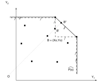
Following Deprins et al. (1984), Daraio and Simar (2007b, p. 34) note that the FDH set is «the union of the all positive orthants in the inputs and of the negative orthants in the outputs whose origin coincides with the observed points in (𝑋_𝑖, 𝑌_𝑖) ∈ 𝜒», being the smallest free disposal set containing all the observed production bundles5_{. Figure}_4.1 provides a stylized representation of a free disposal hull production set, compared to a convex PPS.

Similar to Equation 4.3, the estimated output requirement is given by:

̂

𝑃 (𝑥)_{𝐹 𝐷𝐻} = {𝑦 ∈ 𝑅𝑞₊|(𝑥, 𝑦) ∈ ̂Ψ_{𝐹 𝐷𝐻}} (4.10)

And the estimated frontier by:

𝐼𝑠𝑜𝑞 ̂𝑃 (𝑥)_{𝐹 𝐷𝐻} = {𝑦|𝑦 ∈ ̂𝑃 (𝑥)_{𝐹 𝐷𝐻}, 𝜆𝑦 ∉ ̂𝑃 (𝑥)_{𝐹 𝐷𝐻}∀𝜆 > 1} (4.11)

The output oriented efficiency measure of a given production bundle (𝑥₀, 𝑦₀) is thus given by the estimated 𝜆_{𝐹 𝐷𝐻}:

̂

𝜆_{𝐹 𝐷𝐻}(𝑥₀, 𝑦₀) = max{𝜆|𝜆𝑦₀ ∈ ̂𝑃_{𝐹 𝐷𝐻}(𝑥₀)} = max{𝜆|(𝑥₀, 𝑦₀) ∈ ̂Ψ_{𝐹 𝐷𝐻}}

(4.12)

Therefore, from Equations4.9 and 4.12, the efficiency scores FDH estimator is given

5_{The estimated FDH expression compares to the DEA convex counterpart, which in} _{Banker et al.}

(1984)is defined as: ̂ Ψ𝐷𝐸𝐴= {(𝑥, 𝑦) ∈ 𝑅 𝑝+𝑞 + |𝑦 ≤ 𝑛 ∑ 𝑖=1 𝛾𝑖𝑌𝑖; 𝑥 ≥ 𝑛 ∑ 𝑖=1 𝛾𝑖𝑋𝑖; 𝑛 ∑ 𝑖=1 𝛾𝑖= 1; 𝛾𝑖≥ 0; 𝑖 = 1, ..., 𝑛}

The difference between the two PPS is given by the weights 𝛾, for which in this case are not binary, being allowed to take values different than either 0 or 1, and endowing the PPF with its convex shape. However, the FDH estimator is a more general estimator of Ψ, as it does not require the convexity assumption.

(31)

Note: 𝐵′ is the radial projection of the production bundle B in the FDH frontier and 𝐵″ is the same type of projection but in a convex DEA frontier. Source: Daraio and Simar (2007b, p.

36)

Figure 4.1: FDH and DEA estimation of 𝑃 (𝑥) and 𝐼𝑠𝑜𝑞𝑃 (𝑥) in a 2-output space.

by: ̂ 𝜆_{𝐹 𝐷𝐻}(𝑥₀, 𝑦₀) = max{𝜆|𝜆𝑦₀ ≤ 𝑛 ∑ 𝑖=1 𝛾_𝑖𝑌_𝑖; 𝑥₀ ≥ 𝑛 ∑ 𝑖=1 𝛾_𝑖𝑋_𝑖; 𝑛 ∑ 𝑖=1 𝛾_𝑖= 1; 𝛾_𝑖 ∈ {0, 1}; 𝑖 = 1, ..., 𝑛} (4.13) ̂

𝜆_{𝐹 𝐷𝐻} is thus the solution to an integer linear program (Daraio and Simar, 2007b, p. 35). For the particular case of a sample 𝜒 of 𝑛 schools, the efficiency of a given school is evaluated by the corresponding estimated score ̂𝜆_{𝐹 𝐷𝐻} computed taking into account the full sample of schools’ inputs and outputs (𝑋_𝑖, 𝑌_𝑖) ∈ 𝜒.

In practical terms, the estimator determines the set of observed production bundles in

̂

Ψ that weakly dominates the production bundle (𝑥₀, 𝑦₀), i.e., that uses at most the same input or produces at least the same output. In the case of a 1-input 1-output production process, the efficiency score is computed with respect to the following weakly dominating set:

𝐷₀ = {𝑖|(𝑋_𝑖, 𝑌_𝑖) ∈ 𝜒, 𝑋_𝑖 ≤ 𝑥₀, 𝑌_𝑖 ≥ 𝑦₀} (4.14)

The efficiency score is thus computed, through an output oriented perspective, as:

̂

𝜆_{𝐹 𝐷𝐻}(𝑥₀, 𝑦₀) = max_𝑖∈𝐷₀(𝑌𝑖

𝑦₀) (4.15)

(32)

by: ̂ 𝜆_{𝐹 𝐷𝐻}(𝑥₀, 𝑦₀) = max_𝑖∈𝐷 0{min𝑗=1,...,𝑞( 𝑌_𝑖𝑗 𝑦𝑗₀)} (4.16)

In which 𝑌_𝑖𝑗 is the quantity of output 𝑗 produced by the dominating school 𝑖, and 𝑦₀𝑗 is the quantity of output 𝑗 delivered by the school under efficiency evaluation, with 𝑌_𝑖, 𝑦₀𝑗 ∈ 𝑅𝑞₊.

The technical efficiency scores of our empirical study are estimated by the FDH method, through Equation 4.16. As in Cordero et al. (2017), it is assumed that schools have the objective to maximize the cognitive abilities of their students and are not able to easily adequate their inputs in the short term. Therefore an output-oriented perspective is taken, where efficiencies are obtained through an expansion of output rather than a reduction of input.

4.3. Controlling for super-efficiency

An important limitation of FDH – and DEA – estimation relates to its deterministic nature. Statistical inference based on envelopment techniques is sensitive to extreme values or outliers (Cazals et al., 2002, p. 3). In particular, it is possible for the efficiency scores to be significantly affected by the existence of outlier ’super-efficient’ production bundles, i.e., observations with abnormally high output quantities or abnormally low input quantities due, for instance, to measurement errors. The existence of a significant number of super-efficient observations in the sample biases the estimation – a production bundle (𝑥₀, 𝑦₀) that would otherwise be efficient reveals an underestimated efficiency score if the dominating set 𝐷₀ exclusively contains units which are super-efficient in the above sense. Parametric methods have been dealing with this problem mainly through maximum likelihood estimation of stochastic frontiers, dividing the error term in inefficiency and random noise (Aigner et al., 1977; Greene, 1980a). However, these require a parametric specification of the production function. On the other hand, non-parametric methods have been tackling this drawback mainly through partial frontier analysis, making use of a statistical version of Ψ.

Our empirical study also controls for super-efficiency by relying on additional partial frontier analysis models, namely order-m and order-𝛼, which are now succinctly described.

(33)

4.3.1.

Order-m estimator

The order-m estimation method was first introduced by Cazals et al. (2002) and, unlike the standard FDH estimator, does not consider the full frontier as the benchmark for the efficiency measurement. The technique consists in enveloping only a subsample of 𝑚 ≥ 1 observations that are randomly drawn with replacement from the set of observations with at least the same level of output.

Since the sub-samples are drawn with replacement, and given the statistical properties of the method, it is possible that a school with production bundle (𝑥, 𝑦) has an efficiency score lower than the estimated partial frontiers’ mean, which implies that ̂𝜆_𝑚(𝑥, 𝑦) < 1, being super-efficient.

The expected order-m frontier can thus be defined as «the expected value of the

maxi-mum of m random variables 𝑌1_{, ..., 𝑌}𝑚 _{drawn from the conditional distribution function}

of 𝑌 given that 𝑋 ≤ 𝑥» (Daraio and Simar, 2007a, p. 81). For the case with multiple

outputs, and for a given number of inputs 𝑥 and 𝑚 i.i.d. random variables 𝑌_𝑖, with 𝑖 = 1, ...𝑚, the PPS can be defined for any 𝑦 as:

̃

𝜆_𝑚(𝑥, 𝑦) = max_{𝑖=1,...,𝑚}{min_{𝑗=1,...,𝑞}(𝑌

𝑗 𝑖

𝑦𝑗)} (4.17)

The expected order-m output efficiency measure, 𝜆_𝑚(𝑥, 𝑦) is thus defined, for all 𝑥 in which the distribution function of 𝑋 is not zero, as:

𝜆_𝑚(𝑥, 𝑦) = 𝐸 ( ̃𝜆_𝑚(𝑥, 𝑦|𝑋 ≤ 𝑥)) = = 𝐸 [max_{𝑖=1,...,𝑚}{min_{𝑗=1,...,𝑞}(𝑌 𝑗 𝑖 𝑦𝑗)} ∣𝑋 ≤ 𝑥] (4.18)

Increasing the number 𝑚 of observations randomly drawn from the sample of 𝑛 schools for partial frontier analysis approximates the efficiency scores from those of the full fron-tier, as the lim_𝑚→∞𝜆_𝑚(𝑥, 𝑦) = 𝜆_{𝐹 𝐷𝐻}(𝑥, 𝑦) . Since the value of the estimator is not bounded, there will be schools which are super-efficient ( ̂𝜆_𝑚(𝑥, 𝑦) < 1), for finite values of 𝑚6_{. Therefore, in empirical applications, the number of super-efficient production units} is dependent on the number 𝑚 the analyst chooses to benchmark each production unit

6_{The order-m estimator is also}√_{𝑛-consistent, assymptotically unbiased and assymptotically normally}

distributed. However, for a study of the assymptotic properties of the order-m estimator please refer to

(34)

with.

The method is then repeated 𝐵 times, thus benchmarking each observation to 𝐵 randomly drawn partial frontiers. The order-m efficiency measure is finally computed as the simple mean of the estimated distances. According to the algorithm in Daraio and Simar (2007a, pp. 82-83) the order-m estimation can be summarized in four steps, namely:

1. From the set of schools that produce at least as much of any output as school 𝑖, a sample of 𝑚 schools is drawn randomly with replacement. 2. Pseudo FDH efficiency scores, ̃𝜆𝑏_𝑚(𝑥, 𝑦), are computed through Equation

4.17.

3. Steps 1 and 2 are repeated 𝐵 times, for 𝑏 = 1, ..., 𝐵, with 𝐵 large. 4. Order-m is computed as the average ̂𝜆_𝑚(𝑥, 𝑦) ≈ 1

𝐵∑ 𝐵 𝑏=1𝜆̃

𝑏

𝑚(𝑥, 𝑦).

The choice of 𝐵 is then a matter of accuracy. The greater the 𝐵 the more accurate will be the approximation, which comes however, at the expense of a larger computation time (Tauchmann, 2011, p. 4).

In economic terms, the interpretation of the estimates should be straightforward. A given school with an estimated order-m efficiency score of 1/𝑧 produces 𝑧 times the esti-mated maximum attainable output from a set of 𝑚 other schools drawn randomly from the empirical sample.

4.3.2.

Order-alpha estimator

Similarly to order-m, Aragon et al. (2005) developed an estimator based on re-sampling techniques, however following a quantile-based approach. According to the order-𝛼 method a given school with production plan (𝑥, 𝑦) is evaluated against the frontier defined by the output level exceeded by (1 − 𝛼) × 100% of the schools that use 𝑥 or lower levels of each input. Following the notation in Tauchmann (2011, p. 4) the output-oriented order-𝛼 estimator can be written as:

̂

𝜆_𝛼(𝑥, 𝑦) = 𝑃_(1−𝛼){min_{𝑗=1,...,𝑞}(𝑌

𝑗 𝑖

𝑦𝑗) ∣𝑋 ≤ 𝑥} (4.19)

Where 𝑃 (1 − 𝛼) denotes the 𝛼 × 100th percentile of schools where 𝑋 ≤ 𝑥. For 𝛼 = 1 the estimator coincides with FDH, while for 𝛼 < 1 some observations will be classified as super-efficient. If ̂𝜆_𝛼(𝑥, 𝑦) = 1 the school is efficient at the 𝛼 × 100% level in the sense that it is dominated by other schools using the same or less input than 𝑥 with only a

(35)

probability of 1 − 𝛼7_.

4.4. Metafrontier approach

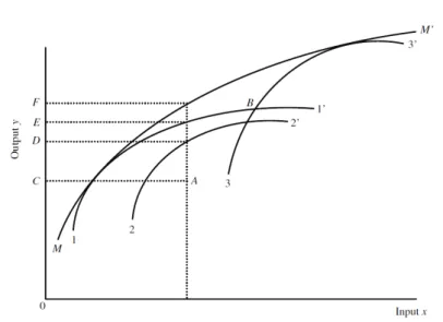
In international analysis of school efficiency – as the one developed here – data are gen-erally hierarchical. Schools can be both evaluated in comparison with other schools oper-ating in the same country or with other schools operoper-ating in different education systems. Extending the approach followed in Portela and Thanassoulis (2001) and Thanassoulis and Portela (2002), and in the spirit ofO’Donnell et al. (2008), two different types of pro-duction frontiers can be estimated: i) 𝑘 local frontiers for the sub-samples of 𝑛_𝑘schools in each 𝑘th country in the full sample; and ii) an international best practice frontier for the whole sample of 𝑛 schools. It is assumed that schools in the same country operate under a similar set of institutional rules than schools from different countries, being therefore submitted to more similar constraints. Therefore, the distance of a given school to its respective local frontier can be conceptualized as the part of the overall efficiency score that can be attributable to school efficiency (ScE), or the country-level efficiency score, while the distance from the local frontier to the international metafrontier can be inter-preted as the country effect (CE) (Cordero et al., 2017, p. 367). Figure 4.2 provides an illustration of a metafrontier enveloping 3 local frontiers in a 1-input 1-output scenario.

Source: O’Donnell et al. (2008, p. 236)

Figure 4.2: Metafrontier illustration with 3 local frontiers

7_{The order-𝛼 estimator has the same statistical properties of the order-𝑚 estimator, i.e., it is}

assymp-totically unbiased, normally distributed and √𝑛-consistent (Aragon et al., 2005). Nevertheless,Daouia and Simar (2007)show that the order-𝛼 method is more robust to extreme values.

(36)

1-B-3’ represents the non-convex metafrontier enveloping the local frontiers, if it is

assumed that these are all the 𝑘 separable groups. Otherwise, the metafrontier can be theoretically conceived as the M-M’ frontier, as there may be other feasible production bundles (O’Donnell et al., 2008, p. 235).

Taking an output-oriented perspective, the efficiency scores resulting from benchmark-ing the inefficient production bundle denoted by A and with output C in Figure4.2against its corresponding local frontier 2-2’ and the international frontier 1-B-3’ can be computed as: 𝜆𝐺𝐸 𝐴 = 0𝐸 0𝐶 (4.20) Where 𝜆𝐺𝐸

𝐴 denotes the global efficiency score of A and 0𝐸 and 0𝐶 the distances

between the origin and coordinates C and E, respectively. On the other hand,

𝜆𝑆𝑐𝐸 𝐴 =

0𝐷

0𝐶 (4.21)

Which is the ratio between the potential output defined by the local frontier and the actual output C.

The country effect of unit A (𝜆𝐶𝐸

𝐴 ) is finally given by:

𝜆𝐶𝐸_𝐴 = 0𝐸 0𝐷 = 0𝐸/0𝐶 0𝐷/0𝐶 = 𝜆𝐺𝐸_𝑖 𝜆𝑆𝑐𝐸 𝑖 (4.22)

From Equation4.22, and generalizing, global efficiency can be easily derived as 𝜆𝐺𝐸 𝑖 =

𝜆𝑆𝑐𝐸

𝑖 × 𝜆𝐶𝐸𝑖 .

4.5. Explaining the variation in school efficiency

After accounting for the decomposition of the global efficiency scores in within-country school efficiency and country effects the relevance of other variables in explaining the dis-tribution of efficiency scores is ensued. Educational activity is influenced by institutional and contextual factors that hinder or catalyse efficient allocations of school resources. The introduction of environmental variables, 𝑧 = (𝑧₁, ..., 𝑧_ℎ) ∈ 𝑅ℎ, in the analysis enables to investigate what is the impact of given factors affecting the organization of school activity on their efficiency in providing quality education. Given the nature of the data used in this study three separate subsets of variables are considered: school characteristics (𝑧𝑠𝑐ℎ𝑙_),