Adolfo Sachsida§ Mario Jorge Cardoso de Mendonça¤ Paulo Roberto Amorim Loureiro†
resumo
Este artigo testa a hipótese de punição salarial contra moradores de regiões pobres. Isto é, nós explicitamente testamos a idéia de que trabalhadores morando em regiões pobres recebem uma punição salarial em relação a trabalhadores similares que moram em regiões ricas. Os resultados econométricos são robustos tanto a um amplo conjunto de variáveis explicativas como também a diferentes especificações econométricas. Estima-dores de 2 e 3 estágios são usados para corrigir tanto o viés de endogeneidade, associado ao local de moradia, como também para a correção do viés associado a ausência de uma proxy adequada para a variável habilidade. Os resultados econométricos sugerem expressiva punição salarial para os moradores de regiões pobres. Além disso, quatro explicações para a correlação entre salários e local de moradia foram testadas. Os resultados fornecem evidências favoráveis a: i) existência de uma relação negativa entre o tempo gasto para se chegar de casa ao trabalho e a produtividade do trabalhador; e b) ocorrência de discriminação estatística contra traba-lhadores que residem em regiões pobres.
Palavras-chave: punição salarial, discriminação espacial, local de residência.
abstract
This article tests the hypothesis of wage punishment against workers living in poor counties. That is, we explicitly test the idea that workers living in poor counts receive a wage punishment in relation to similar skilled workers living in rich counties. The econometric results are robust to both a large set of explanatory variables and different econometric specifications. The 2 Stages and the 3 Stages Least Squares approach are used to correct both the endogeneity of the place of residence and the omission of the variable ability (ability bias). After all, the results suggest expressive wage punishment against workers that lived in poor areas. Fur-thermore, four alternative explanations for the correlation between wages and place of residence are tested and the results provide evidence in favor of i) a link between time spent commuting to workplace and productivity of the worker; and ii) statistical discrimination against workers that live in poor areas.
Keywords: wage punishment, spatial discrimination, place of residence.
JEL classification: J71, J31.
* Os autores agradecem aos participantes do XXIX Encontro Brasileiro de Econometria, bem como a dois pareceristas anônimos, por comentários e sugestões que em muito contribuíram para a qualidade deste trabalho. Eventuais erros e/ou omissões permanecem de inteira responsabilidade dos autores.
§ Catholic University of Brasília and IPEA. Address to correspondence: Catholic University of Brasília, SGAN 916, Mo-dulo B, Sala A-118, 70790-160 Brasília, DF. E-mail: [email protected].
1 i
ntroductionStudies that relate wage differences to the existence of discrimination in the labor market
are common in economics [Becker (1957), Phelps (1972), inter alia]. However, recent studies
have expanded such literature to include important topics in such discussions. These works seem to show that the discrimination phenomenon is not limited to solely the race or sex of the individual, but can also expand to include people of the same race and sex. Physical appearance [Hamermesh and Biddle (1994)], physically handicaps [Famulari (1992)], height [Persico and Postlewaite (2004)] or even the place of residence [Kain (1968)] have become new variables that may incite some kind of wage discrimination against an individual.
Wage or job opportunity punishment may occur for several reasons. One reason is that statistical discrimination may occur. For example, if an individual lives in a neighborhood kno-wn to house a certain type of people (poor people, for example), the employer may associate the characteristics of people from that area to the individual in question, thus reducing his chances of being contracted, or earning a higher wage. Secondly, discrimination by preference could take place. This means that the employer simply does not like people that live in certain neigh-borhoods (or cities). Thirdly, a person may have poor job opportunities if the Spatial Mismatch Hypothesis (SMH) exists which states that individuals who live far from their workplaces have
difficulty accessing the best job opportunities [Kain (1968)].1 Lastly, there is some economic
ra-tionality to the fact that wages are related to the dwelling place of the individual. For example, people who live far from their workplaces might spend more time and energy in traffic, thus reducing their capacity to produce once in the job.
The objective of this article is to verify the effect of the place of residence over an individual’s wage. Furthermore, the different explanations that can cause this result are tested. It is important to stress that to complete this study the construction of a new data set was neces-sary. The econometric results indicate severe wage punishment against workers living in poor counties. More than that, the econometric evidence suggests that both the statistical discrimi-nation and the economic rationale expladiscrimi-nation cannot be ruled out. Besides this introduction, section 2 presents a detailed description of the dataset. Section 3 presents the econometric re-sults. Lastly, section 4 describes the conclusions of the article.
2 d
atasetThe dataset refers to the Distrito Federal State, which lies in the central count of Brazil. According to the 2000 census data from the Brazilian Institute of Geography and Statistics, the population of the Distrito Federal was 2,051,146 inhabitants who are spread throughout 19 administrative counts. Due to budget limitations, this research was limited to 4 of these
ties: Brasília (population: 198,422), Taguatinga (population: 243,575), Sobradinho (population 128,789) and Ceilândia (population 344,039). As a group, these 4 counties equal 44.6% of the population of the Distrito Federal State.
Table 1 shows the distribution of the population of the Distrito Federal States in its diffe-rent administrative counties in 2000. They are listed according to population size. Also shown is the Index of Human Development (IDH), the average annual income per capita and per family, and the average family size.
Table 1 – Administrative counts of the Distrito Federal State*
Administrative Count Population % IDH Average Annual
Income per capita
Average Size of
Families
Average Annual
Income per family
Ceilândia 344,039 16.8 .784 2,217 4.32 9,575
Taguatinga 243,575 11.9 .853 4,818 4.20 20,236
Brasília 198,422 9.7 .936 10,890 3.75 40,837
Samambaia 164,319 8.0 .781 2,251 4.27 9,613
Planaltina 147,114 7.2 .764 1,832 4.20 7,696
Gama 130,580 6.4 .815 2,756 4.13 11,382
Sobradinho 128,789 6.3 .837 3,395 4.10 13,918
Guará 115,385 5.6 .867 6,404 4.07 26,063
Santa Maria 98,679 4.8 .794 1,373 4.57 6,277
Rec. Das Emas 93,287 4.5 .775 1,392 4.29 5,971
São Sebastião 64,322 3.1 .820 1,610 4.14 6,667
Cruzeiro 63,883 3.1 .928 7,529 4.02 30,266
Paranoá 54,902 2.7 .785 1,343 4.31 5,788
Brazlândia 52,698 2.6 .761 1,904 4.30 8,187
Riacho Fundo 41,404 2.0 .826 2,808 4.40 12,353
N. Bandeirante 36,472 1.8 .898 5,852 3.90 22,823
Lago Norte 29,505 1.4 .933 15,910 4.17 66,344
Lago Sul 28,137 1.4 .945 21,389 3.87 82,777
Candangolândia 15,634 0.8 .853 3,387 4.23 14,325
Distrito Federal 2,051,146 100 .849 4,518 4.15 18,750
* the population data comes from the census data elaborated by the Brazilian Institute of Geography and Statistics in the year of 2000. The data about income (in 1997 US$ values), the size of family and IDH come from the Distrito Federal Company to Development (CODEPLAN).
(home of the President of the Republic), the ministries, etc.; b) Taguatinga and Ceilândia are the most populous and important areas in the south of Brasília (an average distance of 20 miles from the center of Brasília); c) Sobradinho is the most populous and important administrative county north of Brasília (around 17 miles from the center of Brasília); and d) these four
popu-lous areas have existed long enough to have their own dynamics.2
Data collection took place during May and June of 2004, in the administrative counties of Brasília, Taguatinga, Ceilândia and Sobradinho. A total of 1,104 people were interviewed. They answered a sixty-question questionnaire regarding socio-economical and behavioral characteristics. To obtain a more homogenous sampling, only people between the ages of 25 and 55 years old were interviewed. Moreover, all the individuals who called themselves public employees (civil or military) were not interviewed due to the fact that the dynamics that ruled their wages was different from that of the market. The average time to complete the form was approximately 7 minutes. The individuals were interviewed in different points in the adminis-trative counties. In addition, the interviewers participated in 8 hours of instruction concerning how to conduct good interviews.
Not all the information collected was used in this article. Furthermore, as is usual in eco-nometric studies, some filters were applied to the sample. Following the standard procedure of literature regarding the return to schooling, individuals who were still studying were excluded also. For the same reason people with an hourly wage of more than R$ 300 (approximately US$ 100) or less than R$ 1.00 were also withdrawn from the sampling. Finally, only individuals with a weekly workload of 36 to 44 hours were included in the sample. As a result of these filters the sampling size was reduced to 799 individuals.
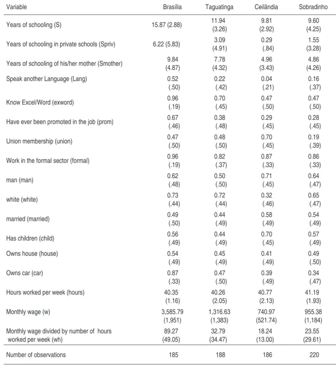
Table 2 presents some descriptive statistics concerning the sample used for this research. The results are separated by administrative counts. For example, an individual who lives in Brasília studies approximately 15.87 years. However, for a resident of Sobradinho, this same measurement is reduced to 9.60. In addition, the number of years of study in private schools is greater for people who live in Brasília than for those who live in other counts. Also, in reference to Table 2, it is noted that 52% of those interviewed who live in Brasília speak a second langua-ge, in contrast to 22% of those who live in Taguatinga, 4% of those residing in Ceilândia and 16% of those in Sobradinho. Another interesting detail is that while 87% of Brasília residents own their own car, this percentage decreases to 39% in Ceilândia and 34% in Sobradinho.
Table 2 – Descriptive statistics*
Variable Brasília Taguatinga Ceilândia Sobradinho
Years of schooling (S) 15.87 (2.88) 11.94
(3.26)
9.81 (2.92)
9.60 (4.25)
Years of schooling in private schools (Spriv) 6.22 (5.83) 3.09 (4.91)
0.29 (.84)
1.55 (3.28)
Years of schooling of his/her mother (Smother) 9.84 (4.87) 7.78 (4.32) 4.96 (3.43) 4.86 (4.26)
Speak another Language (Lang) 0.52
(.50) 0.22 (.42) 0.04 (.21) 0.16 (.37)
Know Excel/Word (exword) 0.96
(.19) 0.70 (.45) 0.47 (.50) 0.47 (.50)
Have ever been promoted in the job (prom) 0.67 (.46) 0.38 (.48) 0.29 (.45) 0.28 (.45)
Union membership (union) 0.47
(.50) 0.48 (.50) 0.70 (.45) 0.19 (.39)
Work in the formal sector (formal) 0.96 (.19) 0.82 (.37) 0.87 (.33) 0.86 (.33)
man (man) 0.62
(.48) 0.50 (.50) 0.71 (.45) 0.64 (.47)
white (white) 0.73
(.44) 0.72 (.44) 0.32 (.46) 0.65 (.47)
married (married) 0.49
(.50) 0.44 (.49) 0.58 (.49) 0.54 (.49)
Has children (child) 0.56
(.49) 0.44 (.49) 0.70 (.45) 0.57 (.49)
Owns house (house) 0.54
(.49) 0.45 (.49) 0.41 (.49) 0.49 (.50)
Owns car (car) 0.87
(.33) 0.47 (.50) 0.39 (.49) 0.34 (.47)
Hours worked per week (hours) 40.35 (1.16) 40.26 (2.05) 40.77 (2.13) 41.19 (1.93)
Monthly wage (w) 3,585.79
(1,951) 1,316.63 (1,383) 740.97 (521.74) 955.38 (1,184) Monthly wage divided by number of hours
worked per week (wh)
89.27 (49.05) 32.79 (34.47) 18.24 (13.00) 23.55 (29.61)
Number of observations 185 188 186 220
* the values in parentheses are the standard deviations of the variables.
3 e
conometricresultsexo-genous variables that measures both human capital and individual characteristics. Mincerian equations are common throughout studies that concern return to schooling [Mincer (1974),
Griliches (1977), Garen (1984), Card (2001), inter alia]. Two problems associated with the use
of mincerian equations in wage estimates are: a) the ability bias (that is, the ability of an indi-vidual is not easily measured – its absence in the model may cause an estimative bias); and b) the endogeneity of the schooling variable. In the construction of the dataset, special attention was give to both these problems. Thus, in the questionnaire, questions were included that cap-tured the “ability” of an individual (if he spoke another language, if he knew how to work with software like Word and Excel, how many years he had studied in private school, how many years his mother had studied and if he had ever been promoted in the job). On the other hand, in an attempt to solve the problem of endogeneity of the education variable, a two-stage least square model was estimated. Later in this text more detail will be provided in regard to these proceedings.
It is important to emphasize that the authors of this article are not concerned about the
return to education.3 The authors utilize a mincerian framework to verify the importance of
the place of residence on individual wages. In this sense, the problems of the omission of the
variable ability and the endogeneity issue must be understood within the scope of this paper. That is, the problem of such “ability bias” lies in the fact that individuals with high amount of ability can receive higher wages and live in richer counties. If this is true, the fact of residence location affecting wages will be a spurious fact, because the true effect will be generated by the ability variable, which was omitted in the equation. In a similar manner, the choice of the place of residence may be endogenous. For example, the individual can choose the place of residence according to his wage, or can even choose to live close to his/her job.
Table 3 shows the results obtained by ordinary least squares (OLS)as well as Two-Stage
least squares (2-LS). In this table, the dependent variable is the logarithm of the monthly wage per hour worked during the week (Lwh). Two groups of explanatory variables have been adopted. In the first group the classic set of variables that appear in the studies on returns to education is utilized. The second group adds the following variables to the previous set: an individual’s ability to speak another language (lang), if the applicant knows how to work with software like Word and Excel (exword), how many years the person studied in private school (Spriv), the number of years of education of the applicant’s mother (Smother), whether or not the individual has ever been promoted (prom), and if he owned his own house (house). The premise is that this new set of variables can possibly isolate the effect of the ability variable,
eliminating (or reducing) the ability bias.A dummy variable was also included which became
a value equal to l (one) if the individual has children and 0 (zero) if not. The justification for the inclusion of this variable is to try to capture the effect of the presence of children on the individual’s wage. To verify the effect of mobility on the individual’s wage, a dummy variable (car) that assumed the value 1 (one) if the individual owned a car was also included in the regression. Finally, in each estimate a count dummy was included which assumed the value
l (one) if the person lived in that count and 0 (zero) if not. Brasília was considered the base county.
Table 3 shows some interesting results on wages, such as the effect of schooling and parti-cularly, private schooling. However, we will focus on the effect of residence location on indivi-dual wages. Even using the wide set of variables (equations 2 and 4), there is strong evidence of the occurrence of wage discrimination due to the place of residence of the individual. Using the full set of variables to capture the idea of ability, the OLS estimation indicates a wage punish-ment of 38 percent for the individuals that live in Taguatinga, 52 percent for the inhabitants of Ceilândia and 58 percent for the inhabitants of Sobradinho. To address the endogeneity problem in the choice of the location to live, the wage equation is re-estimated by two-stages least squares (the place of residence is the endogenous variable and we use the following set of exogenous variables: smother, race, smoke, drink, kids, and wage). The 2-LS regression shows no wage penalty against the inhabitants of Taguatinga, but strong wage punishment for the inhabitants of both Ceilândia and Sobradinho.
Table 3 – Preliminary estimative on the relation between place of residence and wages*
Dependent Variable: Lwh OLS 2-LS**
(1) (2) (3) (4)
S .1446
(21.99)
.0881 (12.56)
.0511 (3.63)
.0291 (1.92)
Experience .0410
(4.99)
.0453 (6.01)
.0708 (4.29)
.0637 (3.99)
Experience^2 -.0004(-2.66) -.0006(-3.90) -.0011(-3.33) -.0011(-3.34)
Formal .0971(1.50) .0725(1.27) .2772(2.14) .2866(2.17)
Union .0091(0.20) -.0293(-0.73) -.1879(-1.60) -.3107(-2.58)
Man .1934(4.68) .1261(3.45) .2936(3.58) .2499(3.03)
White .0647
(1.52)
-.0128 (-0.34)
-.1466 (-1.37)
-.1586 (-1.48)
Married .2135
(4.95)
.1469 (3.48)
.3035 (4.17)
.1876 (2.24)
Spriv .0221
(4.77)
.0022 (0.23)
Smother .0023(0.51) -.0281(-2.85)
Lang .1843(3.77) .2480(2.42)
Exword .0851(1.74) -.0264(-0.27)
Prom .3007(7.55) .2325(3.01)
Child -.0172
(-0.38)
.0437 (0.46)
House .0691
(1.83)
.2565 (3.37)
Car .3685
(8.60)
.2183 (2.53)
Taguatinga -.5378(-8.65) -.3827(-6.85) -.6484(-1.75) -.3247(-0.85)
Ceilândia (-10.48)-.7506 -.5281(-8.06) -2.109(-8.16) -1.818(-6.27)
Sobradinho (-11.69)-.7665 -.5864(-9.78) (-11.58)-2.741 (-10.14)-2.674
Constant 1.178(7.93) 1.334(9.82) 2.889(8.16) 3.018(8.12)
R2 Adj. .6847 .7613 .1242 .1115
Number of observations 779 778 778 777
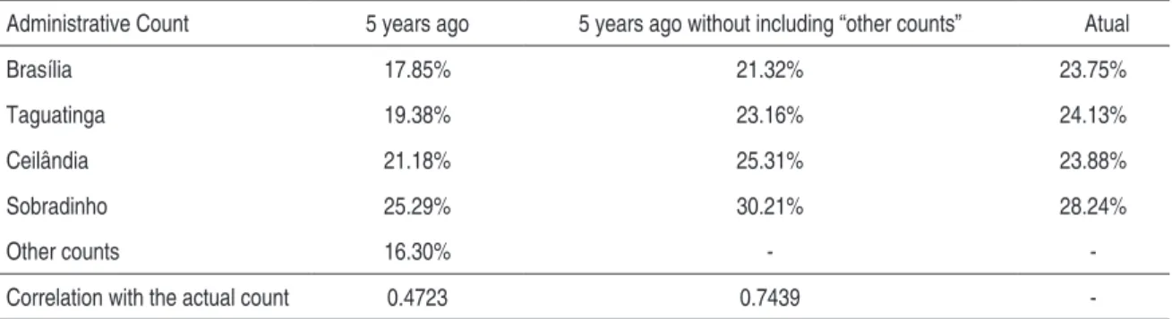
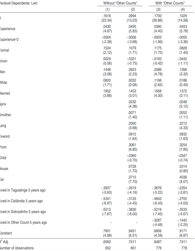
In the questionnaire there is the following question: “In what administrative county did you live 5 years ago?” One would not expect that the count a person lived in 5 years ago would bear influence on the error term of the wage equation. Nevertheless, if there is a high correla-tion between where an individual lived 5 years ago and where he presently lives, this variable can be used as a proxy for the place of residence. Table 4 describes a distribution of individuals by current place of residence and that of 5 years ago. An important detail is that, 5 years ago, some people lived in a county outside the counties studied here. Such people were grouped in the group “other counties”. Column 1 describes the distribution of the place of residence 5 years ago. Column 2 describes the same variable, without taking into account the “other counties” group. Column 3 describes the current distribution. Finally, the last line of Table 4 describes the correlation between the place of residence 5 years ago and the present dwelling place. As indicated by this table, there is a significant correlation between the locations of past and pre-sent residences. For example, in the case where “other counties” is not included the correlation is 0.74.
Table 4 – Distribution of individuals according to their past and present place of residence
Administrative Count 5 years ago 5 years ago without including “other counts” Atual
Brasília 17.85% 21.32% 23.75%
Taguatinga 19.38% 23.16% 24.13%
Ceilândia 21.18% 25.31% 23.88%
Sobradinho 25.29% 30.21% 28.24%
Other counts 16.30% -
-Correlation with the actual count 0.4723 0.7439
Table 5 – Estimate on the relation between place of residence 5 years ago and wages*
Variável Dependente: Lwh Without “Other Counts” With “Other Counts”
(1) (2) (3) (4)
S .1616
(23.34) .0994 (13.03) .1700 (26.86) .1029 (14.58) Experience .0430 (4.67) .0495 (5.83) .0380 (4.40) .0453 (5.78) Experience^2 -.0004 (-2.38) -.0006 (-3.68) -.0003 (-1.86) -.0005 (-3.36)
Formal .1524
(2.12) .1079 (1.71) .1175 (1.72) .0828 (1.40) Union .0029 (0.06) -.0331 (-0.75) -.0193 (-0.42) -.0442 (-1.11)
Man .1448(3.08) .0923(2.23) .2086(4.78) .1266(3.32)
White .0820(1.71) .0032(0.08) .1166(2.65) .0188(0.49)
Married .1902(3.86) .1453(3.01) .1958(4.30) .1372(3.11)
Spriv .0232 (4.38) .0248 (5.12) Smother .0071 (1.40) .0052 (1.11) Lang .2050 (3.68) .2212 (4.33) Exword .0912 (1.64) .0832 (1.63)
Prom .3061(6.85) .3254(7.85)
Child -.0360(-0.70) -.0347(-0.74)
House .0728(1.70) .0314(0.80)
Car .3715(7.70) .4036(9.07)
Lived in Taguatinga 5 years ago -.3937 (-5.63) -.2619 (-4.19) -.3676 (-5.22) -.2354 (-3.81)
Lived in Ceilândia 5 years ago -.5341
(-6.97) -.3133 (-4.45) -.4843 (-6.43) -.2705 (-4.03)
Lived in Sobradinho 5 years ago -.5513 (-7.87) -.3830 (-6.00) -.5219 (-7.45) -.3533 (-5.67)
Lived in Other Count 5 years ago - - -.3287(-4.48) -.1442(-2.25)
Constant .7901 (4.98) .9451 (6.51) .6806 (4.59) .9171 (6.87)
R2 Adj. .6562 .7411 .6487 .7411
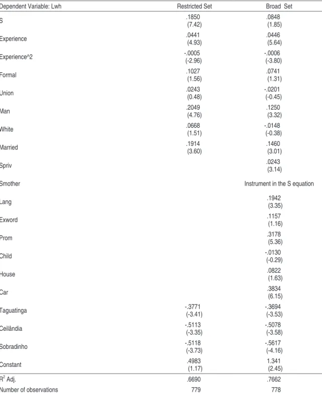
According to Tables 3 and 5, there is little doubt that there is an actual wage differential caused by an individual’s place of residence. To verify this result, the results gathered from 3 Stage Least Squares (3LS) are shown in Table 6. In this table, there are two dependent varia-bles: Lwh and S. For Lwh, the use of the two previous sets of explanatory variables is conti-nued. For S, following explanatory variables are used: Smother, man, white, married, Tagua-tinga, Ceilândia and Sobradinho. The novelty of this regression is that now there is an attempt to control the endogeneity of years of study. To save space, we will just report the results for the
equation of the greatest interest, which is the wage equation.4
The results presented in Table 6 leave no doubt concerning the occurrence of a signifi-cant wage punishment for the residents of Taguatinga (37 percent), Ceilândia (51 percent) and Sobradinho (56 percent). The remaining results are similar to those shown in the previous regressions. After detecting the difference in wages, generated by the place of residence, it now remains for us to try to propose an explanation for this differential. As mentioned in the introduction of this article, there are at least 4 possible explanations for such a fact: 1) Spatial Mismatch Hypothesis (SMH); 2) economic rationale; 3) statistical discrimination; and 4) pre-ference discrimination.
According to the Spatial Mismatch Hypothesis (SMH) some groups of individuals (due to their race, ethnic background, creed, etc.) are not allowed to rent houses in city suburbs where the best job opportunities can be found. As a result, these individuals must live in counties far from better job opportunities and consequently are not able to compete for the best jobs and higher wages. For example, Blacks could possibly have difficulty renting or buying residences in certain neighborhoods where the majority of residents are white. Therefore, they would be for-ced to live in other areas. If the better job opportunities are in white neighborhoods, there may be a greater distance between where Blacks actually live and where the best jobs are actually located. Such a situation makes it difficult for Blacks to get better employment, resulting in: a) different wages for blacks and whites; and b) different wages caused by the place of residence.
According to the above paragraph, SMH provides an explanation for the wage differential resulting from the places of residence. However, SMH is fundamentally based upon the fact that discrimination against some groups of individuals exists in the real estate market. Perhaps this is a reasonable hypothesis for some counties in the United States. But it definitely does not apply to the real estate market in the Distrito Federal State. A brief glance at the data in Table 2 verifies this conclusion. Note that in the sampling, 73% of those interviewed in Brasília were white. In Taguatinga that percentage was 72%, in Ceilândia, it was 32% and in Sobradinho, the percentage of whites was 65%. Percentage-wise, it is apparent that the white population in Taguatinga is almost the same as in Brasília. Furthermore, Sobradinho (the county which has the greatest magnitude of discrimination) possesses a white population very similar to that of Brasília and double that of Ceilândia. To accept the SMH we must not recognize a wage diffe-rential between the Brasília and Taguatinga counties and, additionally, the wage diffediffe-rential
must be much more severe in Ceilândia than in Sobradinho. These facts are not in accordance with the results found in this study.
Table 6 – Estimative by 3LS*
Dependent Variable: Lwh Restricted Set Broad Set
S .1850(7.42) .0848(1.85)
Experience .0441(4.93) .0446(5.64)
Experience^2 -.0005(-2.96) -.0006(-3.80)
Formal .1027(1.56) .0741(1.31)
Union .0243
(0.48)
-.0201 (-0.45)
Man .2049
(4.76)
.1250 (3.32)
White .0668
(1.51)
-.0148 (-0.38)
Married .1914(3.60) .1460(3.01)
Spriv .0243(3.14)
Smother Instrument in the S equation
Lang .1942(3.35)
Exword .1157
(1.16)
Prom .3178
(5.36)
Child -.0130
(-0.29)
House .0822(1.63)
Car .3834(6.15)
Taguatinga -.3771(-3.41) -.3694(-3.53)
Ceilândia -.5113(-3.35) -.5078(-3.58)
Sobradinho -.5118
(-3.73)
-.5617 (-4.16)
Constant .4983
(1.17)
1.341 (2.45)
R2 Adj. .6690 .7662
Number of observations 779 778
An important detail worth mentioning is that in the great majority of cases, there are two options when renting houses in the Distrito Federal state. One option is to prove income and present 2 co-signers (people who will be held responsible for paying the rent if the renter does not). One of the co-signers must own property in the Distrito Federal state. The second option is to prove income and pay a down payment equivalent to 6 months rent (this money is retur-ned at the end of the contract). In other words, there is not much room for discrimination if the individual fulfills one of the prerequisites cited above. However, in some instances, it may be argued that salespeople were unfair in regards to certain groups of people. Nevertheless, in the Distrito Federal state, a great part of the real estate is announced in newspapers and websites that include photos. This reduces the dependence that an individual may feel toward the real estate agent. Furthermore, to rent property the salesman almost never accompanies the real estate clients. The practice is that the client chooses the property they want to visit and picks up the keys at the agency (leaving some I.D at the real estate company). The client then inspects the selected property alone, without the presence of the real estate broker. Thus, the possibility of discrimination occurring in the real estate market in the Distrito Federal is quite remote, which eliminates the SMH as a possible explanation for the wage differential amongst the counties in the Distrito Federal.
Table 7 – Time spent to arrive at workplaces and means of transportation
Variable Brasília Taguatinga Ceilândia Sobradinho
Time spent to workplace (in minutes)
Standard Deviation (in minutes)
Lower and Upper time spent (in minutes)
% that spent more than 40 minutes
% that spent less than 20 minutes
14.92
8.25
2 – 50
2.7%
87.9%
36.57
20.89
3 – 100
44.9%
29.4%
37.17
23.97
1 – 120
47.9%
34.9%
34.81
16.57
5 – 100
50.5%
28.1%
Percentage traveling by car 68.1% 36.1% 22.1% 26.8%
Percentage traveling by bus 11.3% 46.8% 61.3% 59.5%
As indicated above, the economics rationale based on commuting costs can explain a sha-re of the wage diffesha-rential between Brasília and the other counties. However, the explanation cannot be used to explain why there is such a great difference between the counts. As shown in Table 7, it is difficult to understand why residents from Sobradinho are less privileged than those living in Taguatinga. After all, these counties have similar statistics regarding the means of transport to work and time spent traveling to the workplace. According to data shown in Table 7, one would expect the greatest wage differential to be found in Ceilândia since the resi-dents of this county spend more time getting to their workplaces and use private transportation less often. In addition, it is unusual that a difference of twenty minutes in the amount of time needed to travel to work would drive the wage differential to the high level reported in Tables 3, 5 and 6.
Discrimination occurring by preference is a possibility that must be examined. For exam-ple, the occurrence of discrimination by preference against Blacks is a common assumption in economic studies since: a) employers do not like Blacks (discrimination by preference of the employer); or b) clients do not like to be assisted by Blacks (discrimination by preference of the client).
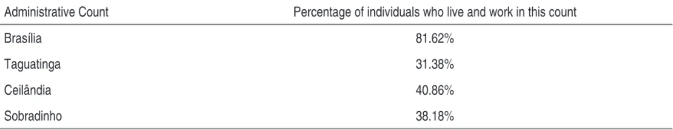
Table 8 – Percentage of individuals who live and work in the same count
Administrative Count Percentage of individuals who live and work in this count
Brasília 81.62%
Taguatinga 31.38%
Ceilândia 40.86%
Sobradinho 38.18%
It makes no sense that blacks will discriminate (by taste or preference) against blacks, or that women will discriminate against women. In the same way, there is no sense in a company located in Taguatinga discriminates against the residents from Taguatinga. Similarly, why would clients who buy products in Taguatinga to discriminate against residents from this coun-ty? If a client chooses to travel to Taguatinga (or Ceilândia or Sobradinho) to buy a product, discrimination against the dwellers of that county makes no sense. After all, if he is willing to travel to that place, he should also is willing to be attended by a resident from that same area. Thus, the greater the percentage of individuals who work and live in the same county, the less discrimination by preference against the residents of that area should be.
Data in Table 8 indicated that 40% of Ceilândia residents also work there. So it seems to be illogical that such people suffer wage discrimination by preference. A similar analysis can be made of Taguatinga and Sobradinho. Observe that, of the 3 counties, Taguatinga is the city showing the smallest percentage of workers living in the same county. Thus it would be logical to expect greatest degree of discrimination by preference against the residents of Taguatinga. The estimates do not support this assumption. It appears that the existence of discrimination by preference is not the most adequate type of discrimination that represents the results.
Finally, one can suggest that the results encountered are due to the occurrence of statistical discrimination. That is, since employers are not completely familiar with the profile of each worker, they attribute to the worker the average characteristics of the group that the worker be-longs. Thus, workers living in Brasília would be classified according to the average residents of Brasila, and the same would apply regarding the residents of Taguatinga, Ceilândia and Sobra-dinho. Therefore, since Brasília is the richest county and has a population boasting the highest level of education, statistical discrimination against the residents of Taguatinga, Ceilândia and Sobradinho in favor of the residents of Brasília is a strong possibility.
In order to verify the hypothesis of statistical discrimination, the following procedure nee-ds to take place. The mincerian equation should be re-estimated with the broad set of variables
by OLS,5 however, just a sub-sample of the original dataset should be used. In our estimates,
only those individuals who work and live in different counties will be included. The rationale for this is that now an employer must contract individuals from different counties. In doing so, he may apply his opinion regarding their group (city of residence) to these individuals. The
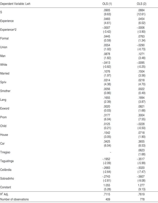
occurrence of discrimination, then, implies statistical discrimination. In the second column of Table 9, our original sampling is used; however, a dummy variable (trregion) that assumes a value of 1 (one) if the individual lives and works in the same count and 0 (zero) otherwise is included. The idea is to verify if this variable is able to change the results found. In other words, the use of the variable will verify the validity of our results. Table 9 presents the results of these procedures.
According to individuals who live in Taguatinga and work outside Taguatinga earn wages that are approximately 19 percent less than the residents of Brasília who work outside Brasília. For Ceilândia and Sobradinho these results are 26 percent and 27 percent, respectively. These percentages indicate the existence of statistical discrimination against the residents of Taguatin-ga, Ceilândia and Sobradinho. These results imply that residents of Brasília working in other
counties, even after the control by a series of variables, receive higher wages than residents of
Taguatinga (or Ceilândia or Sobradinho) working in other counties. Therefore, a resident of Braslia working in Taguatinga receives higher wages than a resident of Taguatinga working in Brasília (even after the control by a wide range of variables). Another important finding is that the inclusion of the dummy variable trregion does not qualitatively alter the results. Note that trregion is positive and statistically significant at a 10% level. This indicates that individuals that live and work in the same count receive a higher wage than individuals that work outside their county of residence. This result can be interpreted as both:
evidence that the productivity model makes sense. That is, the fact that the individual •
lives and works in the same place would save travel time and energy of the worker making him more productive and, consequently, able to receive a higher wage; or
evidence in favor of the statistical discrimination model. That is, when the employer •
Table 9 – Mincerian regression for people who work and live in different counts*
Dependent Variable: Lwh OLS (1) OLS (2)
S .0905
(9.63) .0884 (12.61) Experience .0483 (4.61) .0454 (6.02) Experience^2 -.0007 (-3.42) -.0006 (-3.90)
Formal .0445
(0.59) .0763 (1.34) Union .0554 (1.02) -.0290 (-0.73) Man .0878 (1.82) .1271 (3.48) White -.0413 (-0.82) -.0095 (-0.25) Married .1076 (1.97) .1504 (3.56) Spriv .0314 (4.38) .0218 (4.70) Smother .0056 (0.86) .0022 (0.49) Lang .1655 (2.39) .1894 (3.87) Exword .0020 (0.03) .0821 (1.68) Prom .3177 (6.04) .3004 (7.55) Child .0125 (0.21) -.0228 (-0.50) House .1542 (3.05) .0718 (1.90) Car .3425 (6.04) .3655 (8.53)
Trregiao - .0623
(1.68) Taguatinga -.1952 (-2.09) -.3517 (-5.99) Ceilândia -.2683 (-2.64) -.5020 (-7.47) Sobradinho -.2743 (-2.81) -.5607 (-9.08) Constant 1.055 (5.28) 1.277 (9.13)
R2 Adj. .7115 .7619
Number of observations 409 778
4 c
onclusionsThis article used an original dataset that provided information for 4 administrative coun-ties in the state of the Distrito Federal in Brazil. Armed with these data a series of econometric procedures were carried out to verify the existence of wage differences resulting from the place of residence of the worker. The econometric results demonstrated to be extremely robust to a wide set of statistical procedures. In addition, all results supported the existence of severe wage punishment against workers that lived in poor areas.
It may be argued that our results are biased since the decision regarding the place of resi-dence is endogenous. Individuals with more skills will possibly migrate to rich areas, and low skilled workers will live in poor areas. Such choices of residence will bias the results in favor of wage differences between areas. To prevent this bias we performed two different econometric procedures. First, we estimated the regressions using two-stage least squares (2-LS). Secondly, we used a proxy that highly correlated with the place of the residence, but was not associated with the actual wage received by the workers. This proxy kept our results qualitatively the same. In other words, our statistical procedure addressed the endogeneity problem.
After finding a statistically significant wage gap between workers from different counties, we proposed four different explanations for this gap. While we did not find strong evidence in favor of both the Spatial Mismatch Hypothesis (SMH) and the discrimination by preference, we did not rule out the explanations based on economic rationale (commuting cost) and statis-tical discrimination.
Although it was showed that part of the wage differential between counties was attributed to factors linked to worker productivity, such as time spent commuting from home to work-place, it was apparent that an important part of this differential was linked to the existence of statistical discrimination against those living in poor counties.
r
eferencesBARBOSA FILHO, F.; PESSÔA, S. Retorno da educação no Brasil. pesquisa e planejamento Econômico,
2008. No prelo.
BECKER, G. The economics of discrimination. The University of Chicago Press, 1957.
BECKER, G. Human capital.ColumbiaUniversity Press, 1975.
BIDDLE, J. I.; Hamermesh, D. Beauty, productivity and discrimination:lawyers’ looks and lucre. Journal
of labor Eonomics, 16, p. 172-201, 1998.
BOARDMAN, J.; FIELD, S. H. Spatial mismatch and racial differences in male joblessness: Cleveland
and Milwaukee, 1990.Sociological Quarterly, v. 43, p. 237-55, 2002.
CAIN, G. The economic analysis of labor market discrimination:a survey. In Ashenfelter, Orley; Layard,
CARD, D. Estimating the return to schooling: progress on some persistent econometric problems. Econo-metrica, v. 69, n. 5, p. 1127-1160, 2001.
FARMULARI, M. The Effects of a Disability on Labor Market Performance: The Case of Epilepsy.
Southern Economic Journal, p. 1072-1087, 1992.
GABRIEL, S.; ROSENTHAL, S. Commutes, Neighborhoods Effects and Earnings: An Analysis of Racial
Discrimination and Compensating Differentials. Journal of urban Economics, v. 40, 1996, p. 61-83.
GAREN, J. The Returns to Schooling: A Selectivity Bias Approach with a Continuous Choice Variable.
Econometrica, v. 52, n. 5, p. 1199-1218, 1984.
GOBILLON, L.; SELOD, H.; ZENOU, Y. Spatial mismatch: from the hypothesis to the theories. London,
2003. (CEPR Discussion Paper , n. 3740)
GREKING, S. D.; WEIRICK, W. N. Compensating differences and interegional wage differentials.
Review of Economics and Statistics, p. 483-487, 1983.
GRILICHES, Z. Estimating the returns to schooling: some econometrics problems. Econometrica, v. 45,
n. 1, p. 1-22, 1977.
GYOURKO, J.; TRACY, J. The importance of local fiscal conditions in analyzing local labor markets.
Journal of political Economy, p. 1208-1231, 1989.
HAMERMESH, D. S.; BIDDLE, J. E. Beauty and the labor market.american Economic Review, v. 84,
p. 1174-1194, 1994.
KAIN, J. F. Housing segregation, negro employment, and metropolitan decentralization. Quarterly Journal
of Economics, v. 82, p. 175-83, 1968.
______. The cumulative impacts of slavery:jim crow, and housing market discrimination on black welfare.
October, 1992. (HEIR Discussion Paper, n. 1608).
KATZ, L. F. Efficiency wages theories: a partial evaluation. NBER, p. 235-276, 1986.
MINCER, J. Schooling, experience and earnings. National Bureau of Economic Research, 1974.
MOURA, R. L. Testando as hipóteses do modelo de Mincer para o Brasil. Revista Brasileira de Economia,
2008. No prelo.
PERSICO, N.; POSTLEWAITE, A. Theeffect of adolescent experience on labor market outcomes: the
case of height. Journal of political Economy, v. 112, n. 5, p. 1019–1053, 2004.
PHELPS, E. S. The statistical theory of racism and sexism.american Economic Review, LXII, p.
659-661, 1972,
RESENDE, M.; WYLLIE, R. Retornos para educação no Brasil: evidências empíricas adicionais. Economia
aplicada, v. 10, n. 3, p. 349-365, 2006.
SACHSIDA, A., LOUREIRO, P. R. A.; MENDONÇA, M. J. C. Um estudo sobre retorno em escolaridade
no Brasil. Revista Brasileira de Economia, v. 58, n. 2, 2004.
SHAPIRO, C.; STIGLITZ, J. Equilibrium unemployment as a worker discipline device. american
Eco-nomic Review, 74, p. 433-444, 1984.