*e-mail: [email protected]
Utilising Neural Networks and Closed Form Solutions to Determine Static Creep
Behaviour and Optimal Polypropylene Amount in Bituminous Mixtures
Serkan Tapkına*, Abdulkadir Çevikb, Şenol Özcana
aCivil Engineering Department, Anadolu University, Eskişehir, Turkey bCivil Engineering Department, University of Gaziantep, Gaziantep, Turkey
Received: March 1, 2012; Revised: May 23, 2012
The testing procedure in order to determine the precise mechanical testing results in Marshall design is very time consuming. Also, the physical properties of the asphalt samples are obtained by further calculations. Therefore if the researchers can obtain the stability and flow values of a standard mixture with the help of mechanical testing, the rest of the calculations will just be mathematical manipulations. Determination of mechanical testing parameters such as strain accumulation, creep stiffness, stability, flow and Marshall Quotient of dense bituminous mixtures by utilising artificial neural networks is important in the sense that, cumbersome testing procedures can be avoided with the help of the closed form solutions provided in this study. Marshall specimens, prepared by utilising polypropylene fibers, were tested by universal testing machine carrying out static creep tests to investigate the rutting potential of these mixtures. On the very well trained data basis, artificial neural network analyses were carried out to propose five separate models for mechanical testing properties. The explicit formulation of these five main mechanical testing properties by closed form solutions are presented for further use for researches.
Keywords: Marshall design, static creep test, bitumen modification, polypropylene fibers, strain accumulation, artificial neural networks, closed form solutions
1. Introduction
The creep test (conducted in an unconfined or confined manner), has been used to estimate the rutting potential of dense bituminous mixtures. This test is conducted by applying a static or a repeated load to an asphalt specimen and measuring the resulting permanent deformation. Extensive studies using the unconfined creep test (also known as simple creep test or uniaxial creep test) as a basis of predicting permanent deformation in dense bituminous mixtures has been conducted up to date. Research of permanent deformation in flexible pavements began in the early 1970’s1-7. The loss of pavement serviceability is a
common result from rutting. A typical serviceability loss occurs when the formation of ruts forces the pavement to crack, which can lead to rapid deterioration of the pavement due to the accumulation of water on the pavement surface. Under normal service conditions, deformations within the bituminous materials occur more frequently during late spring, summer and early fall because of elevated temperature conditions.
To solve this rutting problem in flexible pavements (and other problems such as fatigue and low temperature cracking), scientists have developed some techniques and methodologies called “asphalt (bitumen) modification”. The most popular bitumen modification technique is polymer modification. To this end, novel binders with
improved rheological characteristics are continuously being developed8-12. The best known form of this bituminous
binder improvement is by means of polymer modification, traditionally used to improve the temperature susceptibility of bitumen by increasing binder stiffness at high service temperatures and reducing the stiffness at low service temperatures13.
It has been found that the creep test must be performed at relatively low stress levels (cannot usually exceed 30 psi (206.9 kPa) and low temperature (cannot usually exceed 104 °F (40 °C)), otherwise the sample fails prematurely3,14,15.
The test conditions consist of a static axial stress, σ, of 100 kPa being applied to a specimen for a period of 1 hour at a temperature of 40 °C. These test conditions were standardized following a seminar in Zurich16. This test is
inexpensive and easy to conduct but the ability of the test to predict performance is extremely questionable17. In place
asphalt mixtures are sometimes prone to truck tire pressures of more than 828 kPa (120 psi) and temperatures higher than 60 °C (140 °F)18. Therefore, the conditions of static
creep test do not closely simulate in-place conditions. The outlet of this part of the study was this major drawback of the static creep tests that have been carried out worldwide up to date19. In order to fulfil this aim, multifilament 3 mm
used to determine the optimal fiber addition amount with the aid of static creep tests undertaken in a completely different fashion than the previous ones. In this manner, the rutting potential of dense bituminous mixtures can be explored in a more complete manner.
The first part of the study reviews available literature published in the last four years on the application of polypropylene fibers in asphalt modification. Then short information on static creep testing of dense bituminous mixtures is presentedspanning in the last two decades about the actual loading simulation efforts being undertaken in the laboratory environment. Next, published literature about artificial neural networks in pavement engineering especially after the year 2005 up to date has been introduced. At this point, strain accumulation and creep stiffness determination of Marshall specimens tested by universal testing machine is being analysed. Then, the application of artificial neural network techniques to propose two separate models for strain accumulation and creep stiffness by utilising the physical properties of standard Marshall specimens such as polypropylene fiber addition amount, specimen height (only for strain accumulation proposal), unit weight, voids filled with asphalt, voids in mineral aggregate, air voids and test loading period (for static creep testing) is being put forward. Furthermore, a general overview about the Marshall design is presented in the next section. Then neural network applications related specifically to the Marshall design in the last decade have been presented. Finally, three other neural network models are being presented which uses the physical properties of standard Marshall specimens such as polypropylene fiber addition amount, specimen height, unit weight, voids filled with asphalt, voids in mineral aggregate and air voids in order to predict the Marshall stability, flow and Marshall Quotient values obtained at the end of mechanical tests. The explicit formulation of these mechanical properties based on the proposed neural network model is obtained and presented for further use for researchers who are working with the same kind of or different bitumen modifiers, needless to say, for similar and specific type of aggregate sources, bitumen, aggregate gradation, mix proportioning, modification technique and laboratory conditions.
2. Available Literature Published in the
Last Four Years on the Application
of Polypropylene Fibers in Asphalt
Modification
Until 2008, many valuable studies have been published about fiber modification of dense bituminous mixtures which can be found in a detailed manner in the relevant literature20.
Tapkın21 has found that the addition of polypropylene fibers
into the asphalt concrete on a dry basis alters the behaviour of the mixture in such a way that, Marshall stability values increase, flow values decrease and the fatigue life increases significantly. Tapkın et al.20,22-24 have also worked on the
addition of polypropylene fibers to the asphalt concrete on a wet basis, and have shown that the most favourable and suitable polypropylene type was multifilament, 3 mm long (M-03 type) which increased the Marshall stability values by
20% as well as the stiffness of the asphalt concrete. Repeated load creep tests under different loading patterns have also shown that the time to failure of fiber modified asphalt specimens under repeated creep loading at different loading patterns increased by 5-12 times versus reference specimens, which is a very significant improvement. In another accompanying study, it was found that polypropylene modification of bituminous binders developed the physical and mechanical properties of the mixture and substantially improved its resistance to permanent deformation. Polypropylene modification also resulted in a saving of 30% in the amount of bitumen, resulting in considerable cost savings19. There are also a number of other studies in
the literature on different applications of polypropylene fiber modification of asphalt concrete in the last decade which deserve attention25-33.
3. Static Creep Testing of Dense Bituminous
Mixtures Spanning in the Last Two
Decades About the Actual Loading
Simulation Efforts
The main outcome of this study was the major drawback of the static creep tests and those that have been carried out worldwide up to date19. Therefore, a completely
different loading pattern and testing temperature was adopted. In this study, first of all, the test temperature was chosen as 50 °C, again just like in repeated creep testing regime to simulate actual in-situ conditions24. A static axial
stress, σ, of 100 kPa was applied to the specimens as a preloading for 10 minutes and after, 500 kPa of loading was applied to the specimens for 1 hour to simulate in-place conditions in a realistic manner19. Also it has to be
mentioned that, in today’s modern pavement engineering practices, there are also other bitumen modifying agents other than polypropylene fibers which need to be tested in actual stress levels (like 100 kPa of preloading and 500 kPa loading level in repeated creep test, not 10 kPa preloading and 100 kPa loading level like the older practices) in order to show the very positive contribution of these modifiers to the genuine mechanical behaviour of modified dense bituminous mixtures.
Matthews and Monismith34 have performed unconfined
creep tests at temperatures 25 °C, 38 °C and 49 °C which is a main departure from the published literature up to date in the testing temperature manner and deserves attention. In another study by Mallick et al.35, in order to
simulate the average pavement temperature throughout the United States, 60 °C of testing temperature was utilised. Ramsamooj and Ramadan36 had carried out creep tests at
four stress levels under constant stresses of 150, 400, 650 and 900 kPa. This was again an important deviation from the accustomed practices of creep testing that deserves attention. Tashman et al.37 had carried out triaxial confined
static creep test in determining the model parameters related to their studies. This is again a significant departure from the routine testing protocol of 40 °C temperature16. A static
differential transformer (LVDT); thus the experimental tertiary creep pattern could not have been recorded naturally. Chen et al.38 had investigated the mechanical responses and
modelling of rutting in flexible pavements. In a recent study, Chen et al.39 investigated the utilization of recycled brick
powder as alternative filler in asphalt mixture. They had carried out static and dynamic creep tests using Universal Testing Machine (UTM) to apply constant stress to asphalt specimens. Their specimens were 100 mm in diameter and 100 mm in height. These specimens were tested at 60 °C with a constant stress of 100 kPa for 3600 seconds and unloaded for the recovery of deformations for 5400 seconds. Also in some studies, in the last five years that was utilising the “standard” procedure depicted in Zurich16, the testing
temperature had been chosen as 30 °C which was again a departure from this technique40-42.
4. Published Literature About Artificial
Neural Network Applications in
Pavement Engineering Especially After
Year 2005 Up to Date
Detailed knowledge about the applications of artificial neural networks in transportation engineering and pavement engineering up to year 2005 can be found in the relevant literature20,43.
Tarefder et al.44 constructed and applied a four-layer
feed-forward neural network to determine a mapping associating mix design and testing factors of asphalt concrete samples with their performance in conductance to flow or permeability. Another study used the artificial neural network methodology to develop time-dependent roughness prediction models for three types of pavements: Portland cement concrete pavement, asphalt overlay over concrete pavement, and asphalt pavement45. Tarefder et al.46
constructed a four-layer neural network and applied this to determine the mapping associating factors in the design and testing of asphalt samples with their performance in repetitive rutting tests. In another study, the concept of a novel neural network-based asphalt compaction analyser capable of predicting the density continuously, in real time, during the construction of the pavement was presented. Preliminary field studies demonstrated the capability of the analyser in predicting the density of an asphalt pavement during construction47. Efforts in
another study had been made to backcalculate the in situ elastic moduli of asphalt pavement from synthetically derived falling weight deflectometer (FWD) deflections at seven equidistant points48. Lacroix et al.49 proposed the
population of a database of measured dynamic moduli with the corresponding predicted resilient moduli to train an artificial neural network. The study by Xiao et al.50
explored the utilization of an artificial neural network in predicting the fatigue life of rubberized asphalt concrete mixtures containing reclaimed asphalt pavement. Xiao and Amirkhanian51 in another look explored the utilization of
the artificial neural networks in predicting the stiffness behaviour of rubberized asphalt concrete mixtures with reclaimed asphalt pavement. A paper by Far et al.52
presented outcomes from a research effort to develop
models for estimating the dynamic modulus (|E*|) of hot-mix asphalt layers on long-term pavement performance test sections. Tapkın et al.20 presented an application of
neural networks for the prediction of repeated creep test results for polypropylene modified asphalt mixtures. Marshall specimens, fabricated with multifilament 3 mm type polypropylene fibers at optimum bitumen content (reference and 3‰ polypropylene fiber modified by weight of aggregate which was not the optimal addition amount according to later studies carried by the lead author19,24)
were tested using universal testing machine in order to determine their mechanical behaviour under repeated creep testing. Different stress values (namely 100, 207 and 500 kPa) and loading patterns (load periods were chosen as 500 ms for all of the specimens and the rest periods were 500, 1000, 1500 and 2000 ms, respectively) have been applied to the previously prepared specimens at 50 °C. It has been shown that the addition of polypropylene fibers results in improved Marshall stabilities and decrease in the flow values, providing the increase of the service life of samples under repeated creep testing (5-12 times when compared to reference specimens). The proposed neural network model uses the physical properties of standard Marshall specimens such as polypropylene type, specimen height, unit weight, voids in mineral aggregate, voids filled with asphalt, air voids and repeated creep test properties such as rest period and pulse counts in order to predict the strain accumulation values obtained at the end of mechanical tests. Moreover parametric analyses have been carried out. The results of parametric analyses were used to evaluate the strain accumulation of the Marshall specimens subjected to repeated load creep tests in a quite well manner. Zhang et al.31 studied polypropylene/waste
ground rubber tire powder composites with respect to the effect of bitumen and maleic anhydride-grafted styrene–ethylene–butylene-styrene content by using the design of experiments approach, whereby the effect of the four polymers content on the final mechanical properties were predicted. Zhang et al.32, this time, studied
waste polypropylene/waste ground rubber tire powder blends with respect to the effect of bitumen and maleic anhydride-grafted styrene–ethylene–butylene–styrene content by using the design of experiments approach, whereby the effect of the four polymer content on the final mechanical properties were predicted. Gopalakrishnan and Manik53 used the falling weight deflectometer data to
determine the in situ mechanical properties (elastic moduli) of the pavement layers through inverse analysis, a process commonly referred to as backcalculation. Tsai et al.54
calibrated mechanistic-based models to field data to produce a design process for predicting reflection cracks. Sakhaeifar et al.55 presented a set of dynamic modulus
(|E*|) predictive models to estimate the |E*| of hot-mix asphalt layers in long-term pavement performance (LTPP) test sections. Tapkın et al.23 presented another application
fibers, fiber contents of 3‰, 4.5‰ and 6‰ by weight of aggregate were utilised and for multifilament 9 mm type and waste fibers only 3‰ fiber content by aggregate weight was utilized which were not the optimal addition amounts according to later studies carried by the lead author19,24) at
bitumen contents varying from 3.5% to 7% (changing by 0.5% increments for 3 specimens at each percentage). It has been shown that the addition of polypropylene fibers results in the improved Marshall stabilities and Marshall Quotient values, which is a kind of pseudo stiffness. The proposed neural network model uses the physical properties of standard Marshall specimens such as polypropylene type, polypropylene percentage, bitumen percentage, specimen height, unit weight, voids in mineral aggregate, voids filled with asphalt and air voids in order to predict the Marshall stability, flow and Marshall Quotient values obtained at the end of mechanical tests. The explicit formulation of stability, flow and Marshall Quotient based on the proposed neural model is also obtained and presented for further use by researchers. Moreover parametric analyses have been carried out. The results of parametric analyses were used to evaluate mechanical properties of the Marshall specimens in a quite well manner. Kargah-Ostadi et al.56 used in a
network-level pavement management system (PMS) to predict future performance of a pavement section and identify the maintenance and rehabilitation needs. There are also various similar studies in the literature in the way of utilising neural networks and parametric studies in various civil engineering applications57-59.
5. Experimental Analysis Carried Out
5.1.
Preparation of the asphalt specimens
Marshall specimens were fabricated by utilising 50 blows on each face (medium traffic conditions). 50/70 penetration bitumen was modified in the laboratory with M-03 type polypropylene fibers. A total of “93” Marshall specimens were fabricated and Universal Testing Machine had been utilised to carry out, this time, to put forward another approach to the rutting prediction of Marshall specimens with carrying out static creep tests on them (the lead author has carried out repeated creep testing with a completely different set of data on another leg of the ongoing studies beforehand20). When compared with the
amount of tests undertaken in the similar studies available in the literature, testing of 93 specimens is really an extensive way of carrying out analyses19,24.
5.2.
Material properties
Gradation limits for wearing course Type 2 set by Highway Technical Specifications of General Directorate of Turkish Highways had been utilised all throughout the studies60. 50/70 penetration bitumen was utilised for the
preparation of the Marshall specimens. The aggregate that had been used throughout the experiments was calcareous type crushed stone. Physical properties of the bitumen samples are given in Table 1. The physical properties of coarse and fine aggregates are given in Tables 2 and 3. The apparent specific gravity of filler is 2785 kg.m–3.
Aggregate gradation had been selected as wearing course type 2 given by General Directorate of Highways of Turkey60. The mixture gradation is given in Table 4.
Physical properties of the polypropylene fibers used in the experimental program are given in the relevant literature24.
Table 1. Physical properties of the reference bitumen.
Property Test Value Standard
Penetration at 25 °C, 1/10 mm 68.35 ASTM D 5-97
Penetration Index –0.26
-Ductility at 25 °C, cm +150 ASTM D 113-99
Specific gravity at 25 °C,
kg.m–3 1028 ASTM D 70-76
Softening point, °C 50.67 ASTM D 36-95
Table 2. Physical properties of coarse aggregates.
Property Test
Value Standard
Bulk specific gravity, kg.m–3 2705 ASTM C
127-04 Saturated surface dry specific
gravity, kg.m–3 2714
ASTM C 127-04
Apparent specific gravity, kg.m–3 2729 ASTM C
127-04
Water absorption, (%) 0.322 ASTM C
127-04 Los Angeles abrasion coefficient (%) 30 ASTM C-131
Table 3. Physical properties of fine aggregates.
Property Test
Value Standard
Bulk specific gravity, kg.m–3 2685 ASTM C
128-04 Saturated surface dry specific
gravity, kg.m–3 2717
ASTM C 128-04
Apparent specific gravity, kg.m–3 2776 ASTM C
128-04
Water absorption (%) 1.236 ASTM C 128-04
Table 4. Type 2 wearing course gradation60.
Sieve size (mm)
Gradation limits (%)
Passing (%)
Retained (%)
12.7 100 100 0
9.52 80-100 90 10
4.76 55-72 63.5 26.5
2.00 36-53 44.5 19.0
0.42 16-28 22 22.5
0.177 8-16 12 10.0
0.074 4-10 7 5
5.3.
Polypropylene modification of bitumen
50/70 penetration bitumen was modified by M-03 type polypropylene fibers. The fibers were premixed with bitumen using a standard mixer at 500 rpm for at least two hours. Mixing temperature was around 165-170 °C61. Only
M-03 type fibers had been utilised to modify the bitumen samples according to the workability criteria22,24. Starting
with 0.5‰ M-03 type, and increasing by 0.5‰ up to 7‰, polypropylene fibers had been premixed with bitumen and were used for preparation of Marshall specimens18. Physical
properties of the polypropylene fiber based bitumen samples with 1 to 7‰ fiber content are given in Table 5.
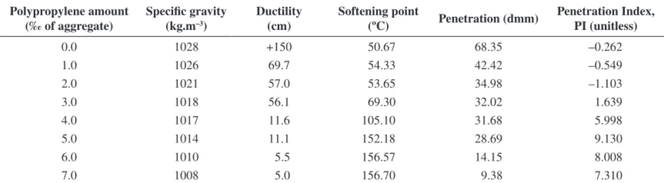
Performance characteristics, such as specific gravity, ductility, softening point, penetration and penetration index of the polypropylene fiber modified bitumen samples were greatly improved as compared to control specimens which can be seen in Table 5. The specific gravity values have decreased by 1.94% when the maximum amount of polypropylene is added to the bitumen samples. Ductility values have dropped to 5.0 cm when 7‰ modification has been carried out. The increase in softening point values is 106.03 °C when compared to control specimens. This is a very remarkable increase from the pavement engineering point of view which is showing the clear decrease in the temperature susceptibility of the bituminous binders with polypropylene fiber modification (tests were carried out in glycerine after 3‰ fiber addition). Penetration values have dropped to 9.38 dmm for 7‰ modification. These above figures altogether show the very positive effect of polypropylene modification to the physico-chemical properties of control specimens according to the temperature susceptibility criteria19.
5.4.
The proportioning of the bituminous
mixtures
To find the optimum bitumen content of reference asphalt specimens, Marshall stability and flow tests were utilised. In order to do this, bitumen contents corresponding to the mixtures with maximal stability and unit weight, 4% air voids and 70% voids filled with asphalt, were found and averaged according to the limits given by the General Directorate of Highways of Turkey60. Two different Marshall
designs were carried out. In the first design, the optimum bitumen content was found as 5%. Second design was ended with an optimum bitumen content of 4.96%. These two
results are very near to each other therefore the optimum bitumen content of the reference specimens has been taken as 5.0%.
6. Experiments Performed to Determine
Optimal Polypropylene Addition to the
Mixture and Artificial Neural Network
Applications by Universal Testing
Machine
6.1.
Static creep tests undertaken
In this study, first of all, the test temperature has been chosen as 50 °C to resemble the in-situ conditions. The height of asphalt specimens was approximately the same for all of the specimens. Prior to testing, the specimens had been placed in an environmental chamber for 24 hours to maintain uniform temperature distribution. Then, the static axial stress,
σ, of 100 kPa was applied to the specimens as a preloading for 10 minutes and after on , 500 kPa of loading was applied to the specimens for 1 hour to resemble in-place conditions in a realistic manner. In order to validate this preloading time of 10 minutes, preloading times of 0 to 10 minutes, increasing one minute by one minute, has been applied to standard Marshall specimens prepared at optimum bitumen content of 5%. A total of 11 specimens had been fabricated and subjected to the same loading pressure of 500 kPa for 1 hour. At the end of these tests, it has been found out that 10 minutes of preloading can be accepted as the optimal preloading time for the further studies that will be carried out with no doubt19. Starting with control specimens (a total of
9 specimens), Marshall specimens have been prepared at the optimum bitumen content of 5% with changing polypropylene contents of 0.5‰ to 7.0‰ by aggregate weight with 0.5‰ increments. For each polypropylene content, a total of 6 specimens have been fabricated. Therefore, in the end, a total of 84 modified specimens have been tested under the static creep test conditions stated above. The mechanical properties of Marshall specimens at the end of static creep tests undertaken by universal testing machine are given in Table 6. These are the average end of test values (preloading [for initial creep stiffness] and actual loading [strain accumulation and final creep stiffness]) obtained for each set of specimens prepared by utilising different polypropylene fiber modification amount. In Figures 1, 2 and 3 these values
Table 5. The physical properties of control and various percentages of polypropylene modified samples.
Polypropylene amount (‰ of aggregate)
Specific gravity (kg.m–3)
Ductility (cm)
Softening point
(ºC) Penetration (dmm)
Penetration Index, PI (unitless)
0.0 1028 +150 50.67 68.35 –0.262
1.0 1026 69.7 54.33 42.42 –0.549
2.0 1021 57.0 53.65 34.98 –1.103
3.0 1018 56.1 69.30 32.02 1.639
4.0 1017 11.6 105.10 31.68 5.998
5.0 1014 11.1 152.18 28.69 9.130
6.0 1010 5.5 156.57 14.15 8.008
are given once more in order to draw the attention to the “optimal” addition of fiber addition. In these three figures, the reader can easily notice the value of 5.5‰ polypropylene fiber addition as the “optimal” addition amount of modifier in a mechanical testing manner.
One can easily notice form Table 6 and Figures 1, 2 and 3 that the addition of polypropylene enhances the mixture properties in a very favourable manner. For example, the control specimens have a final strain accumulation value of 7433.89 µε. On the other hand, the 6‰ polypropylene modified specimens have a final strain accumulation value of 2964.50 µε. This corresponds to a decrease of approximately 60% and deserves attention. On the other hand, the initial
and final stiffness (creep stiffness) values are 83.46 and 67.99 MPa respectively. When the 6‰ polypropylene modified specimens are investigated, these values are 191.65 and 169.15 MPa respectively. These values correspond to an increase of 129% in the initial and 149% in the final creep stiffness values and must be highlighted19.
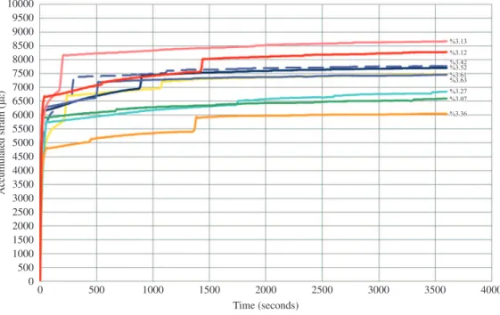
In order to give samples for the strain accumulation versus time graphs of the specimens subjected to creep loading, reference, 3.0‰, 5.5‰ and 7.0‰ modified specimens’ curves (with various air void values) are given below in Figures 4 to 7.
6.2.
Background on artificial neural networks
The operation of the neuron is a complicated and not fully understood process, although the basic details are relatively clear. The neuron accepts many inputs, which are all added up in some manner. If enough active inputs are received at once, then the neuron will be activated and transmit a signal; otherwise the neuron will remain in its inactive quiet state. The influence of the synapses, coupled with the incoming signal into the soma (cell body), can be modelled by a linear combination of the inputs to the processing unit. The more influential the synapse, the larger the signal, the less influential the synapse, the smaller the signal.This basic model, which is analogous to a biological neuron, is shown in Figure 8.
This model, which is called a perceptron simply performs a weighted sum of inputs (a linear combination), compares this to a threshold value in the processing unit and turns on if this value is exceeded, otherwise it stays off. Since the inputs are passed through the model neuron to produce the output once, the system is known as a feed forward one43.
The artificial neuron consists of three main components namely as weights, bias, and an activation function (Figure 8). Each neuron receives inputs x1, x2, ...xn, attached with a weight wi which shows the connection strength for
Figure 2. Initial creep stiffness versus polypropylene amount in static creep tests undertaken.
Figure 3. Final creep stiffness versus polypropylene amount in static creep tests undertaken.
Table 6. Mechanical properties of Marshall specimens at the end of static creep tests undertaken by universal testing machine.
Polypropylene (‰) (by weight of
aggregate)
Accumulated Strain
(µε)
Initial creep stiffness
(MPa)
Final creep stiffness
(MPa)
0 7433.89 83.46 67.99
0.5 5944.00 103.44 84.05
1 5321.33 115.53 95.09
1.5 4888.00 117.48 101.45
2 4594.67 133.37 110.16
2.5 4434.00 134.4 112.18
3 4210.33 135.17 118.2
3.5 4026.83 149.95 124.6
4 3818.83 156.97 132.43
4.5 3547.67 169.8 141.15
5 3171.33 184.72 159.75
5.5 3055.17 209.17 168.98
6 2964.50 191.65 169.15
6.5 3636.50 161.43 137.75
7 3609.83 174.18 139.72
that input for each connection. Each input is then multiplied by the corresponding weight of the neuron connection. A bias bi can be defined as a type of connection weight with a constant nonzero value added to the summation of inputs.
1
H i ij j i
j
u w x b
=
=∑ + (1)
The summation ui is transformed using a scalar-to-scalar function called an “activation or transfer function”, F(ui)
yielding a value called the unit’s “activation”, given in Equation 2.
( )
i i
Y=f u (2)
Activation functions serve to introduce nonlinearity into neural networks which makes artificial neural networks so powerful. The activation function is also referred to as a squashing function.
Neural networks are commonly classified by their network topology, (i.e. feedback, feedforward) and learning
Figure 4. Strain accumulation versus time graphs of the specimens subjected to creep loading of reference specimens’.
or training algorithms (i.e., supervised, unsupervised). For example a multilayer feed forward neural network with back propagation indicates the architecture and learning algorithm of the neural network. Backpropagation algorithm is used in this study which is the most widely used supervised training method for training multilayer neural networks due to its simplicity and applicability. It is based on the generalized delta rule and was popularized by Rumelhart et al.62.
The performance of an artificial neural network model mainly depends on the network architecture and parameter settings. One of the most difficult tasks in artificial neural network studies is to find this optimal network architecture which is based on determination of numbers of optimal layers and neurons in the hidden layers by trial and error approach. The assignment of initial weights and other related
parameters may also influence the performance of the neural network in a great extent. However there is no well defined
Figure 6. Strain accumulation versus time graphs of the specimens subjected to creep loading of 5.5‰ modified specimens’.
rule or procedure to have optimal network architecture and parameter settings where trial and error method still remains valid. This process is very time consuming.
Various back propagation training algorithms which are used in this part of the study is given in Table 7. MATLAB Neural Network Toolbox63 randomly assigns the
initial weights for each run each time which considerably
changes the performance of the trained neural network even all parameters and neural network architecture are kept constant. This leads to extra difficulties in the selection of optimal network architecture and parameter settings. To overcome this difficulty a program has been developed in MATLAB which handles the trial and error process automatically. The program tries various number of layers and neurons in the hidden layers both for first and second hidden layers for a constant epoch for several times and selects the best neural network architecture with the minimum MAPE (Mean Absolute % Error) or RMSE (Root Mean Squared Error) of the testing set, as the training of the testing set is more critical. For instance a neural network architecture with 1 hidden layer with 7 nodes is tested 10 times and the best neural network is stored where in the second cycle the number of hidden nodes is increased up to 8 and the process is repeated. The best neural network for cycle 8 is compared with cycle 7 and the best one is stored as best neural network. This process is repeated n times where n denotes the number of hidden nodes for the first hidden layer. This whole process is repeated for changing number of nodes in the second hidden layer. Moreover this selection process is performed for different back propagation training algorithms such as trainlm, trainscg and trainbfg given in Table 7. The program begins with simplest neural network architecture i.e. neural network with 1 hidden node for the first and second hidden layers and ends up with optimal neural network architecture. The flowchart of the whole process can be found in relevant literature64.
6.3.
Numerical application
Throughout this part of the study, artificial neural networks had been utilised in order to predict the strain accumulation and creep stiffness of asphalt concrete specimens obtained from a series of Marshall designs based on experimental results described above. The ranges for these test results are shown respectively in Tables 8 and 9. The data set is properly divided into 80% training and 20% testing sets for neural network training process and these sets
Table 7. Back propagation training algorithms used in neural network training.
MATLAB function
name
Algorithm
trainbfg BFGS quasi-Newton back propagation
traincgf Fletcher-Powell conjugate gradient back propagation
traincgp Polak-Ribiere conjugate gradient back propagation
traingd Gradient descent back propagation
traingda Gradient descent with adaptive linear back propagation
traingdx Gradient descent w/momentum & adaptive linear back propagation
trainlm Levenberg-Marquardt back propagation trainoss One step secant back propagation
trainrp Resilient back propagation (Rprop) trainscg Scaled conjugate gradient back propagation
Table 8. Ranges of experimental database for strain accumulation analyses.
PP(‰) SpecimenHeight (mm)
Unit Weight (kg.m–3)
Vf (%) V.M.A.
(%) Va (%)
Loading time (seconds)
Accumulated Strain
(µε)
Maximum 7.00 60.80 2465.29 76.89 17.76 6.40 3600.00 8670.00
Minimum 0 57.90 2380.7 62.03 14.84 3.07 0 0
Mean 3.39 59.31 2427.59 69.79 16.14 4.55 1804.57 4208.10
Std. Dev. 2.21 0.62 22.51 3.98 0.78 0.89 1040.47 1327.87
Table 9. Ranges of experimental database for creep stiffness analyses.
PP(‰) Unit Weight
(kg.m–3) Vf (%) V.M.A. (%) Va (%)
Loading time (seconds)
Stiffness (MPa)
Maximum 7.00 2465.29 76.88 16.72 5.21 3596.00 197.20
Minimum 0 2410.78 66.72 14.84 3.07 20.00 57.76
Mean 1.75 2448.71 73.62 15.42 3.72 1835.27 96.62
Std. Dev. 2.61 15.09 2.83 0.52 0.59 1046.68 33.42
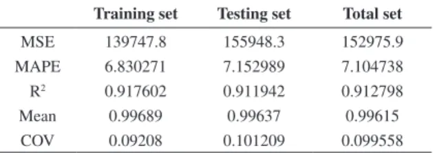
are randomly selected from the experimental database. The optimal neural network architectures for strain accumulation and creep stiffness were found to be 7-9-1 (9 hidden neurons) and 6-8-1 (8 hidden neurons). The optimum training algorithm was found to be Levenberg-Marquardt back propagation. Logarithmic sigmoid (log) and hyperbolic tangent sigmoid (tanh) transfer functions were utilised for the hidden layer and output layer respectively (on a log-log, log-tanh, tanh-log & tanh-tanh basis). It had been clearly seen and proven that there were very minute differences when these four combinations were utilised therefore logarithmic sigmoid transfer function had been used in all throughout the analyses that had been carried out through the study. Statistical parameters of training and testing sets and overall results of neural network models are represented respectively in Tables 10 and 11. As can be visualised from these tables, the obtained neural network results are observed to be markedly close to actual test results. This is a perfect indication of the well training of the data set.
Artificial neural network applications are treated as black-box applications in general. However this study opens this black box and introduces the neural network application in a closed form solution65. This part of the study aims to
present the closed form solutions of proposed neural network models for strain accumulation and creep stiffness based on the trained artificial neural network parameters (weights and biases) as a function of physical properties of standard Marshall specimens such as fiber addition amount, specimen height (only for strain accumulation analysis), unit weight, voids filled with asphalt (Vf), voids in mineral aggregate (V.M.A.), air voids (Va) and test loading period (for static creep testing).
Using weights and biases of the trained neural network model, closed form of strain accumulation can be given as follows:
STRAIN ACCUMULATION (µε) = (sigmoid (–5.12679 × HL_0 + 3.53406 × HL_1 + 0.618816 × HL_2 + 1.37854 × HL_3 + 2.78113 × HL_4 – 9.66212 × HL_5 – 1.96141 × HL_6 + 0.790685 × HL_7 + 2.24663 × HL_8 + 6.73615)
– 0.1)/9.22722e-05) (3)
where;
•HL_0 = sigmoid (–0.84116 × IN_0 – 0.708825 × IN_1 + 0.278111 × IN_2 – 1.35109 × IN_3 – 0.220246 × IN_4 – 0.398603 × IN_5 – 15.4466 × IN_6 + 0.434251);
• HL_1=sigmoid(–5.45661×IN_0+3.2241×IN_1– 5.73856 × IN_2 – 5.08163 × IN_3 + 2.09586 × IN_4 + 2.7223 × IN_5 + 0.26963 × IN_6 – 3.72559); • HL_2=sigmoid(6.5444×IN_0+6.03502×IN_1
+ 3.91636 × IN_2 + 4.05 × IN_3 – 7.78236 × IN_4 – 8.08599 × IN_5 – 0.327217 × IN_6 – 3.99581); • HL_3=sigmoid(–7.44745×IN_0+5.08814×IN_1
– 2.5396 × IN_2 – 4.04074 × IN_3 + 2.40696 × IN_4 + 2.72665 × IN_5 + 0.312135 × IN_6 + 0.369007); • HL_4=sigmoid(7.21775×IN_0–1.15178×IN_1–
2.82139 × IN_2 – 3.10945 × IN_3 – 0.970166 × IN_4 – 0.370003 × IN_5 – 0.134513 × IN_6 – 3.96387); • HL_5=sigmoid(35.5367×IN_0+5.41185×IN_1
– 0.561274 × IN_2 – 0.0351946 × IN_3 – 1.79171 × IN_4 – 1.35406 × IN_5 – 0.571007 × IN_6 – 1.58336);
• HL_6=sigmoid(4.59725×IN_0+2.80553×IN_1 + 0.474659 × IN_2 + 0.888513 × IN_3 – 3.97172 × IN_4 – 3.97018 × IN_5 – 0.748713 × IN_6 – 3.54919);
• HL_7=sigmoid(–9.17083×IN_0–3.3053×IN_1 + 0.857393 × IN_2 + 0.12739 × IN_3 + 0.809459 × IN_4 + 0.852527 × IN_5 + 0.342881 × IN_6 + 2.51807);
• HL_8=sigmoid(–1.23761×IN_0–2.54284×IN_1 + 4.15965 × IN_2 + 3.59557 × IN_3 – 1.44468 × IN_4 – 1.36997 × IN_5 – 0.0352614 × IN_6 + 2.89333) and;
• IN_0=PP(‰)×0.114286+0.1;
• IN_1=SpecimenHeight(mm)×0.275862–15.8724; • IN_2=UnitWeight(kg.m–3) × 0.00945682 – 22.4138;
• IN_3=Vf(%)×0.0538577–3.24079; • IN_4=V.M.A.(%)×0.273786–3.96271; • IN_5=Va(%)×0.240545–0.638713;
• IN_6=Loadingtime(seconds)×0.000222222+0.1 and;
( )
11 x
sigmoid x e− =
+
On the other hand, using weights and biases of the trained neural network model, closed form of creep stiffness can be given as follows:
CREEP STIFFNESS (MPa) = (sigmoid (–0.610361 × HL_0 + 0.313557 × HL_1 + 2.94854 × HL_2 – 1.16768 × HL_3 + 2.92609 × HL_4 + 5.50622 × HL_5 – 2.74787 × HL_6 – 4.74226 × HL_7 –0.130341) + 0.231383)/0.00573723 (4) where;
• HL_0=sigmoid(–0.112266×IN_0–0.774179× IN_1 – 1.06802 × IN_2 – 0.143327 × IN_3 – 0.272591 × IN_4 – 0.403391 × IN_5 – 0.926482);
• HL_1=sigmoid(–0.75386×IN_0+0.213694×IN_1 – 0.0189454 × IN_2 – 1.69661 × IN_3 – 0.834712 × IN_4 – 1.88374 × IN_5 – 0.604095);
• HL_2=sigmoid(0.635743×IN_0+2.37817×IN_1 + 2.38668 × IN_2 – 2.17432 × IN_3 – 2.14612 × IN_4 – 1.26599 × IN_5 – 0.312843);
Table 10. Statistical parameters for strain accumulation analyses.
Training set Testing set Total set
MSE 139747.8 155948.3 152975.9
MAPE 6.830271 7.152989 7.104738
R2 0.917602 0.911942 0.912798
Mean 0.99689 0.99637 0.99615
COV 0.09208 0.101209 0.099558
Table 11. Statistical parameters for creep stiffness analyses.
Training set Testing set Total set
MSE 30.30005 41.73852 39.45083
MAPE 5.072501 5.361045 5.303336
R2 0.968983 0.964309 0.964818
Mean 0.986983 0.986989 0.986988
• HL_3=sigmoid(–0.430883×IN_0–1.3352×IN_1 – 0.572735 × IN_2 + 0.190007 × IN_3 + 0.315196 × IN_4 – 0.625573 × IN_5 – 0.712933);
• HL_4 = sigmoid (–0.605011 × IN_0 + 4.58219 × IN_1 + 5.42914 × IN_2 – 7.95264 × IN_3 – 8.17845 × IN_4 + 0.175617 × IN_5 – 3.58115);
• HL_5 = sigmoid (–0.903958 × IN_0 – 0.634469 × IN_1 – 0.684313 × IN_2 – 0.180382 × IN_3 + 0.639131 × IN_4 – 11.8783 × N_5 – 0.199066); • HL_6=sigmoid(–5.91826×IN_0+3.64127×IN_1
+ 3.65701 × IN_2 – 6.15733 × IN_3 – 6.15846 × IN_4 + 0.210041 × IN_5 – 2.95975);
• HL_7=sigmoid(–6.67541×IN_0+3.1271×IN_1 + 4.26139 × IN_2 – 3.91875 × IN_3 – 3.61073 × IN_4 – 0.589359 × IN_5 – 0.283938);
and;
• IN_0=PP(‰)×0.114286+0.1;
• IN_1=UnitWeight(kg.m–3) × 0.0146754 – 35.2791;
• IN_2=Vf(%)×0.0786884–5.14988; • IN_3=V.M.A.(%)×0.424891–6.20496; • IN_4=Va(%)×0.373303–1.04641;
• I N _ 5 = L o a d i n g t i m e ( s e c o n d s ) × 0.000223714 + 0.0955257;
and;
( )
11 x
sigmoid x e− =
+
7. Experiments Performed to Determine
Optimal Polypropylene Addition to the
Mixture and Artificial Neural Network
Applications by Utilising Marshall Design
7.1.
General overview about Marshall design
The very basic fundamentals for carrying out Marshall design were developed by Bruce Marshall, who was a pavement engineer working for the Mississippi State Highway Department, in the time spanning the period just before the onset of the Second World War in attempt to standardise a testing procedure that would encompass the available laboratory equipment in order to evaluate the bitumen content of asphalt concrete mixtures66,67. In
1948, The U.S. Corps of Engineers, after carrying out elaborate testing practices, improved and built up the certain milestones to Marshall’s test procedure and set the very basic criteria for this very well known hot mix asphalt concrete design method66. Since this time, Marshall
design has been adopted by organisations and government departments in nearly all of the countries worldwide with very minute modifications either to the procedure or to the interpretations of the results. The very basic efforts and the later developments that were carried out in order to standardise this very well known testing procedure and further knowledge can be found in the relevant literature67.
Aggregate selection basically depends on the gradation specifications of the proposed country and available materials in the nearby quarries. Maximum size of aggregate is generally controlled by the layer thickness. Bitumen grade selection is also a very important factor in the overall design
procedure and is again controlled by the requirements of the project66.
Marshall test consists of the manufacture of cylindrical specimens 102 mm in diameter and 63.5 mm high by the use of a standard compaction hammer and a cylindrical mould (further correction factors will be applied to Marshall stability values with different height values). Marshall specimens are compacted using the compactive effort applicable to the loading conditions. These compactive efforts are mainly 35 blows per each face for light traffic, 50 blows for medium and 75 blows for heavy traffic conditions66. A 4.535 kg
hammer is being dropped from 45.72 cm height. After passing of 24 hours from the demoulding of the asphalt specimens, these specimens are tested for their resistance to deformation at 60 °C at a constant rate of 50.8 mm/min in a test rig. The jaws of the loading rig confine the majority but not the entire circumference of the specimen. The top and the bottom of the cylinder are unconfined. Because of this fact, the stress distribution in the specimen during testing is extremely complex68.
Basically, two mechanical properties are determined from the asphalt specimens from the standard Marshall test. These are:
a) The maximum load the specimen will carry before failure, which is known as the Marshall stability, b) The amount of deformation of the specimen before failure occurred, which is known as the Marshall flow.
The ratio of stability to flow is known as the Marshall quotient. Marshall quotient is a sort of pseudo stiffness which is a measure of the material’s resistance to permanent deformation. More scientifically speaking, Marshall quotient is a sort of measure for the creep stiffness of asphalt specimens69.
By carrying out Marshall design procedure, the main goal is to obtain the optimum bitumen content. In order to find the optimum bitumen content, the designer has to find the below mentioned values from the test property curves.
From these data curves, bitumen contents are determined which yields the following:
a) Maximum stability, b) Maximum unit weight, c) The median of limits for per cent air voids, d) The median of limits for voids filled with asphalt.
tool to help them in their pursuits of finding the “optimal” modifier addition amount.
The theory behind the stability, flow and Marshall Quotient values obtained from Marshall testing have been investigated by many scientists up to date in many respects67.
As this study is dealing with preparing an asphalt mixture which has an aggregate gradation of a type 2 wearing course60, at this point, some more “technical” information
about the actual meaning of stability and flow should be given. In pavement engineering, the “stability” of a flexible pavement structure is one of the most remarkable properties. Basically, if the “surface course” is being analysed, the ability of the pavement structure to withstand the distress parameter of rutting is extremely important. The measure of “stability” is not an easy concept on site therefore the laboratory measured value of “stability” gives a good indication of the concept in a qualitative manner. There are minimum values stated for stability values in all of the design guides throughout the world60,66 but there is not any
“maximum” value stated in these guides. If a bituminous mixture is lacking stability, this causes the flow and unravelling of the surface courses of the road infrastructure. Flow is the ability of a bituminous pavement structure to adjust itself to the gradual settlements and movements of the underlying subgrade. It can be accounted for as the reverse of the stability values. Asphalt concrete is a viscoelastic, thermoplastic and viscoplastic material which has “elastic” therefore “reversible” behaviour reserved inside its structure. The Marshall Quotient, another important outcome of the Marshall design procedure, is actually stability divided by flow. Therefore it represents a value of the load to deformation under the specified testing conditions that can be utilised as the measure of the asphalt concrete’s resistance to permanent deformation under service conditions70.
7.2.
Neural network applications related
specifically to Marshall design in the five
years
There are not so many studies in the literature related specifically to neural network applications in Marshall design. Study by Hejazi et al.27 introduced two simple
models for predicting fiber-reinforced asphalt concrete (FRAC) behaviour during longitudinal loads. In this study, an artificial neural network architecture was selected to identify the effect of fiber parameters (as input neurons) on the FRAC properties (specific gravity, stability, and flow as output neurons). MATLAB software was used to implement the algorithm63. Alavi et al.71 derived a high-precision model
to predict the flow number of dense asphalt mixtures using a novel hybrid method coupling genetic programming and simulated annealing, called GP/SA. Mirzahosseini et al.72
presented two branches of soft computing techniques, namely multi expression programming (MEP) and multilayer perceptron (MLP) of artificial neural networks for the evaluation of rutting potential of dense asphalt-aggregate mixtures. Gandomi et al.73, in another study, utilised a
promising variant of genetic programming, namely, gene expression programming (GEP), to predict the flow number of dense asphalt-aggregate mixtures.
7.3.
Experimental analysis carried out
Marshall specimens (at the optimum bitumen content of 5%) were fabricated by utilising 50 blows on each face (medium traffic conditions). 50/70 penetration bitumen was modified in the laboratory with M-03 type polypropylene fibers. A total of “90” Marshall specimens were fabricated and tested to obtain the relevant stability and flow properties of them. When compared with the amount of tests undertaken in the similar studies available in the literature, first of all testing of 90 specimens is really an extensive way of carrying out analyses. Second, in this study, all of the specimens had been prepared by utilising optimum bitumen content therefore a search for “optimal” polypropylene addition amount is undertaken19. Finally, this
time, another way of analysing the Marshall specimens is carried out by knowing the best type of modifier is 3 mm multifilament polypropylene fibers therefore the picture is clearer when compared to the previous studies of the lead author22,23. Average physical and mechanical properties of
six replicate Marshall specimens can be found in Table 12 and Figures 9 to 15.
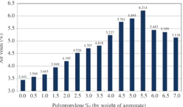
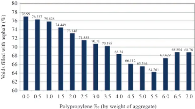
When Table 12 and Figures 9 to 15 are examined, it can be visualized that the average stability values of the control specimens increase up to 70% when 7‰ polypropylene modification is carried out. This is a dramatic increase when viewed from the pavement engineering point of view. The unit weight values drop by 2.9% until 5.5‰ polypropylene amount is reached and after this point on, tends to increase again. The air voids increase by 80% until
Figure 9. Unit weight versus polypropylene amount in Marshall testing.
decrease). Finally, Marshall Quotient values increase by 92% which is an indication of pseudo stiffness. At the end
of the Marshall stability and flow tests, the physical and mechanical properties of the 15 sets of specimens show the optimal polypropylene addition of 5.5‰ in a perfect manner with no doubt19.
7.4.
Numerical application
In this part of the study, artificial neural networks had been utilised in order to predict the stability, flow and Marshall Quotient of asphalt concrete specimens obtained from a series of Marshall designs based on experimental results described above. The ranges for these test results are shown respectively in Tables 13 to 15. The data set is properly divided into 80% training and 20% testing sets for neural network training process and these sets are randomly selected from the experimental database. The optimal neural network architectures for stability, flow and Marshall Quotient found to be 6-8-1 (8 hidden neurons), 6-3-1 (3 hidden neurons) and 6-10-1 (10 hidden neurons) respectively. The optimum training algorithm was found to be Levenberg-Marquardt back propagation. Logarithmic sigmoid (log) and hyperbolic tangent sigmoid (tanh) transfer functions were utilised for the hidden layer and output layer respectively (on a log-log, log-tanh, tanh-log & tanh-tanh basis). It had been clearly seen and proven that there were very minute differences when these four combinations were utilised therefore logarithmic sigmoid transfer function had been used in all throughout the analyses that had been carried out through the study. Statistical parameters of training and testing sets and overall results of neural network models are represented respectively in Tables 16 to 18. As can be visualised from these tables, the obtained neural network results are observed to be markedly close to actual test results. This is a perfect indication of the well training of the data set.
This part of the study aims to present the closed form solutions of proposed neural network models for stability, flow and Marshall Quotient (MQ) based on the trained artificial neural network parameters (weights and biases) as a function of the physical properties of standard Marshall specimens such as fiber addition amount, specimen height, unit weight, voids filled with asphalt (Vf), voids in mineral aggregate (V.M.A.), and air voids (Va).
Using weights and biases of the trained neural network model, closed form of stability can be given as follows:
Figure 12. Voids in mineral aggregate versus polypropylene amount in Marshall testing.
Figure 13. Stability versus polypropylene amount in Marshall testing.
Figure 14. Flow versus polypropylene amount in Marshall testing. Figure 11. Voids filled with asphalt versus polypropylene amount in Marshall testing.
5.5‰ polypropylene amount, and start to decrease from thereon. Voids filled with asphalt values show a similar trend (16.5% decrease) up to 5.5‰ polypropylene addition. The voids in mineral aggregate values increase by 16.4% up to 5.5‰ addition of polypropylene and start to decrease from this point on. The tendency of flow values is similar (23%
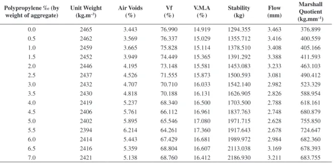
Table 12. Average physical and mechanical properties of six replicate Marshall specimens19.
Polypropylene ‰ (by weight of aggregate)
Unit Weight (kg.m–3)
Air Voids (%)
Vf (%)
V.M.A (%)
Stability (kg)
Flow (mm)
Marshall Quotient (kg.mm–1)
0.0 2465 3.443 76.990 14.919 1294.355 3.463 376.899
0.5 2462 3.569 76.337 15.029 1355.712 3.416 400.559
1.0 2459 3.665 75.828 15.114 1378.510 3.408 405.166
1.5 2452 3.949 74.449 15.365 1391.292 3.388 411.593
2.0 2446 4.195 73.148 15.581 1453.083 3.233 463.103
2.5 2437 4.526 71.555 15.873 1500.593 3.081 490.412
3.0 2432 4.707 70.710 16.033 1542.140 2.982 523.329
3.5 2430 4.818 70.188 16.131 1626.905 2.826 588.954
4.0 2419 5.237 68.340 16.500 1703.500 2.788 618.161
4.5 2406 5.761 66.112 16.961 1837.763 2.748 680.879
5.0 2402 5.895 65.546 17.080 1971.715 2.628 755.850
5.5 2394 6.214 64.261 17.360 1917.643 2.678 724.647
6.0 2414 5.443 67.429 16.681 1989.972 2.984 682.360
6.5 2416 5.359 68.804 16.607 2113.038 3.169 678.393
7.0 2421 5.138 68.760 16.412 2186.930 3.211 683.755
Table 13. Ranges of experimental database for stability analyses.
PP(‰) Specimen
Height (mm)
Unit Weight
(kg.m–3) Vf (%) V.M.A.(%) Va(%) Stability (kg)
Maximum 7.00 62.40 2462.98 87.76 18.64 12.89 2091.04
Minimum 2.50 58.70 2308.04 29.96 15.23 2.18 658.36
Mean 4.75 60.05 2401.60 63.30 16.89 6.27 1297.54
Std.Dev. 1.46 0.80 43.84 19.35 0.90 3.47 355.99
Table 14. Ranges of experimental database for flow analyses.
PP (‰) Specimen
Height (mm)
Unit Weight
(kg.m–3) Vf (%) V.M.A. (%) Va (%) Flow (mm)
Maximum 7.00 62.40 2462.98 87.76 18.64 12.89 7.50
Minimum 2.50 58.70 2308.04 29.96 15.23 2.18 1.35
Mean 4.75 60.05 2401.60 63.30 16.89 6.27 3.65
Std.Dev. 1.46 0.80 43.84 19.35 0.90 3.47 1.49
Table 15. Ranges of experimental database for Marshall Quotient analyses.
PP (‰) Specimen
Height (mm)
UnitWeight (kg.m–3)
Vf (%) V.M.A. (%) Va (%) MQ
(kg.mm–1)
Maximum 7.00 62.40 2462.98 87.76 18.64 12.89 1011.23
Minimum 2.50 58.70 2308.04 29.96 15.23 2.18 89.977
Mean 4.75 60.05 2401.60 63.30 16.89 6.27 427.6827
Std.Dev. 1.46 0.80 43.84 19.35 0.90 3.47 204.68
STABILITY (kg) = (sigmoid (–2.85312 × HL_0 + 3.50241 × HL_1 + 0.693694 × HL_2 – 2.3612 × HL_3 – 5.96018 × HL_4 – 2.94366 × HL_5 – 1.77347 × HL_6 + 0.955348 × HL_7 + 0.963915) + 0.267624) / 0.000558394 (5)
where;
• HL_0 = sigmoid (– 3.82665 × IN_0 + 3.69328 ×
IN_1 – 1.77243 × IN_2 – 3.60365 × IN_3 – 0.15278 × IN_4 + 3.85342 × IN_5 + 1.47133);
• HL_1=sigmoid(–6.68906×IN_0–0.714414×
• HL_2 = sigmoid (– 0.442648 × IN_0 – 0.463069 × IN_1 – 0.674572 × IN_2 – 0.857841 × IN_3 – 0.944217 × IN_4 – 0.645257 × IN_5 – 0.685148); • HL_3=sigmoid(–0.875356×IN_0+2.37839×
IN_1 – 2.09752 × IN_2 – 1.38374 × IN_3 + 0.502376 × IN_4 – 0.029264 × IN_5 – 1.6171);
• HL_4=sigmoid(4.73341×IN_0+1.16066×IN_1 – 0.536602 × IN_2 + 3.55452 × IN_3 + 0.399726 × IN_4 – 9.92582 × IN_5 – 7.38222);
• HL_5 = sigmoid (– 0.325236 × IN_0 + 2.5358 × IN_1 + 4.53548 × IN_2 + 3.10884 × IN_3 – 8.67336 × IN_4 – 3.47159 × IN_5 – 0.823053);
• HL_6 = sigmoid (–5.81405 × IN_0 – 7.87192 × IN_1 + 5.54268 × IN_2 – 4.68907 × IN_3 – 8.83667 × IN_4 + 6.6447 × IN_5 + 6.39212);
• HL_7=sigmoid(–0.86131×IN_0–0.509798× IN_1 –0.731354 × IN_2 – 0.335346 × IN_3 – 1.20513 × IN_4 – 0.810519 × IN_5 – 0.292189);
and;
• IN_0=PP(‰)×0.177778–0.344444;
• IN_1=SpecimenHeight(mm)×0.216216–12.5919; • IN_2=UnitWeight(kg.m–3) × 0.00516334 – 11.8172;
• IN_3=Vf(%)×0.0138402–0.314645; • IN_4=V.M.A.(%)×0.234585–3.47267; • IN_5=Va(%)×0.0747037–0.0625922; and;
( )
11 x
sigmoid x e− =
+
Using weights and biases of the trained neural network
model, closed form of flow can be given as follows: FLOW (mm) = (sigmoid (1.40605 × HL_0 – 1.8657 × HL_1 – 5.88613 × HL_2 + 5.42616) + 0.0761301)/0.130081 (6) where;
• HL_0=sigmoid(0.661376×IN_0+1.35691×IN_1
– 1.24361 × IN_2 + 0.379872 × IN_3 – 0.166156 × IN_4 – 2.30716 × IN_5 – 2.34366);
• HL_1=sigmoid(–2.1095×IN_0+1.19362×IN_1
– 0.174053 × IN_2 – 1.19404 × IN_3 – 2.29043 × IN_4 + 1.35705 × IN_5 + 0.269718);
• HL_2 = sigmoid (–5.04182 × IN_0 – 1.366 ×
IN_1 + 0.264156 × IN_2 – 3.26263 × IN_3 + 0.793789 × IN_4 + 9.26902 × IN_5 + 7.13485);
and;
• IN_0=PP(‰)×0.177778–0.344444;
• IN_1=SpecimenHeight(mm)×0.216216–12.5919; • IN_2=UnitWeight(kg.m–3) × 0.00516334 – 11.8172; • IN_3=Vf(%)×0.0138402–0.314645;
• IN_4=V.M.A.(%)×0.234585–3.47267; • IN_5=Va(%)×0.0747037–0.0625922
and;
( )
11 x
sigmoid x e− =
+
Using weights and biases of the trained neural network model, closed form of Marshall Quotient can be given as follows:
MARSHALL QUOTIENT (kg.mm–1) = (sigmoid (–4.39067
× HL_0 – 0.506972 × HL_1 + 1.60212 × HL_2 + 3.77559 × HL_3 – 2.64216 × HL_4 – 1.52329 × HL_5 – 0.619627 × HL_6 – 1.14162HL_7 – 1.35756 × _HL_8+0.122526 × HL_9+0.512638) – 0.0218674)/0.000868384 (7) where;
• HL_0 = sigmoid (4.63124 × IN_0 + 0.383709 ×
IN_1 + 0.0675933 × IN_2 + 3.08201 × IN_3 + 0.61449 × IN_4 – 8.07108 × IN_5 –5.6658);
• HL_1=sigmoid(–0.6536×IN_0+0.316093×IN_1
– 0.18555 × IN_2 – 0.524093 × IN_3 – 0.853896 × IN_4 – 0.167481 × IN_5 – 1.48732);
• HL_2=sigmoid(0.854237×IN_0–1.70666×IN_1
– 0.139871 × IN_2 + 1.46185 × IN_3 + 0.158078 × IN_4 – 1.55945 × IN_5 – 0.543224);
• HL_3 = sigmoid (– 4.13557 × IN_0 + 3.21316 ×
IN_1 – 5.64472 × IN_2 – 4.26587 × IN_3 + 1.2735 × IN_4 + 1.64707 × IN_5 – 3.90052);
• HL_4 = sigmoid (– 1.54034 × IN_0 – 3.58559 ×
IN_1 – 2.55409 × IN_2 – 2.17112 × IN_3 + 1.28119 × IN_4 + 1.91876 × IN_5 – 0.863922);
• HL_5 = sigmoid (– 0.229126 × IN_0 – 1.2162 ×
IN_1 + 3.01671 × IN_2 + 0.694795 × IN_3 – 4.71187 × IN_4 – 1.01355 × IN_5 – 0.0618821);
• HL_6=sigmoid(–0.521105×IN_0+0.51452×
IN_1 – 0.526448 × IN_2 – 0.437312 × IN_3 – 1.26558 × IN_4 – 0.335999 × IN_5 – 1.11954);
• HL_7=sigmoid(–1.10727×IN_0–0.803725×
IN_1 – 1.79471 × IN_2 – 1.46323 × IN_3 + 0.612343 × IN_4 + 0.633158 × IN_5 – 1.04172);
Table 16. Statistical parameters for stability analyses.
Training
set Testing Set Total set
MSE 9012.055 16590.17805 15074.55
MAPE 5.740424 7.770717044 7.364658
R2 0.933433 0.87581671 0.876589
Mean 0.981275 0.982957961 0.982621
COV 0.077611 0.095206125 0.091563
Table 17. Statistical parameters for flow analyses.
Training set Testing Set Total set
MSE 0.224571 0.21911665 0.22348
MAPE 11.29454 12.3539274 11.50642
R2 0.896754 0.86018833 0.892615
Mean 1.01807 1.02010665 1.018477
COV 0.133298 0.16433526 0.139065
Table 18. Statistical parameters for Marshall Quotient analyses.
Training set Testing Set Total set
MSE 3598.054082 10427.29406 4963.90208
MAPE 11.89680203 14.33756427 12.3849545
R2 0.901771645 0.756157896 0.86973649
Mean 0.985490699 0.974365805 0.98326572
• HL_8 = sigmoid (– 1.0431 × IN_0 + 1.65191 × IN_1 + 0.558663 × IN_2 – 0.40391 × IN_3 – 2.4571 × IN_4 – 0.651791 × IN_5 – 0.689734);
• HL_9=sigmoid(–0.743853×IN_0–0.347985× IN_1 – 0.350831 × IN_2 – 0.26865 × IN_3 – 0.52416 × IN_4 – 0.951561 × IN_5 – 1.1319);
and;
• IN_0=PP(‰)×0.177778–0.344444;
• IN_1=SpecimenHeight(mm)×0.216216–12.5919; • IN_2=UnitWeight(kg.m–3) × 0.00516334 – 11.8172;
• IN_3=Vf(%)×0.0138402–0.314645; • IN_4=V.M.A.(%)×0.234585–3.47267; • IN_5=Va(%)×0.0747037–0.0625922; and;
( )
11 x
sigmoid x e− =
+
It has to be mentioned that the fluctuations in the
flow values (therefore in Marshall Quotient values which are actually stability values divided by flow values) are actually causing the difference between R2 values of the
training and testing sets of Marshall Quotient analyses (Table 18). This is expectable in a clear manner. But to avoid such underperformances, in the prospective studies, the database can be divided into three subsets i.e. train, valid and test though this is not a must (at this point, in the further researches that will be carried out with especially different type of bitumen modifiers, extensive laboratory testing should have to be carried out to arrive at optimal addition amounts of the modifiers of course).
For further recommendations to other researchers studying in the field, static creep tests can be carried out on the polypropylene fiber modified specimens at temperatures above or below 50 °C and with different loading patterns. Another prospective study may focus on the behaviour of the polypropylene modified asphalt specimens at lower temperatures below zero. Different compaction techniques like gyratory compaction might be utilised for the better simulation of site conditions in laboratory environment. Finally, other intelligent predictive tools such as genetic programming74,75 and neuro-fuzzy techniques might be
utilised to give a deeper insight to the proposed problem of determination of the optimal modifier amount in the dense bituminous mixtures.
8. Conclusions
The addition of the polypropylene fibers into the asphalt mixture enhances the mixture properties in a very favourable
manner. The decrease of the strain accumulation at the end of the static creep tests correspond to approximately 60%. The initial and final creep stiffness values have increased by 129% and 149% correspondingly. The average stability values of the control specimens increase up to 70% when 7‰ polypropylene modification is carried out. This is a dramatic increase when viewed from the pavement engineering point of view. The unit weight values drop by 2.9% until 5.5‰ polypropylene amount is reached and after this point on, tends to increase again. The air voids increase by 80% until 5.5‰ polypropylene amount, and start to decrease from thereon. Voids filled with asphalt values show a similar trend (16.5% decrease) up to 5.5‰ polypropylene addition. The voids in mineral aggregate values increase by 16.4% up to 5.5‰ addition of polypropylene and start to decrease from this point on. The tendency of flow values is similar (23% decrease). Finally, Marshall Quotient values increase by 92% which is an indication of pseudo stiffness.
Therefore the 5.5‰ M-03 type polypropylene fiber addition is the optimal addition amount for this type of wet modification. Furthermore, in this study, a novel approach to enable the prediction of mechanical properties such as strain accumulation, creep stiffness, stability, flow and Marshall Quotient without carrying out real destructive tests, obtained from Marshall designs, have been presented utilising artificial neural networks. Backpropagation neural networks have been utilised for the neural network training process. The proposed neural network models for five of these mechanical properties have shown very good agreement with experimental results. But it has to be born in mind that this neural network model is valid for the ranges of the experimental database used for neural network modelling. Therefore, the rutting potential can be explored by this means in a perfect manner. As a consequence, the proposed neural network model and formulation of the available stability, flow and Marshall Quotient of asphalt samples is quite accurate, fast and practical for use by other researchers studying in this field. The explicit formulation of strain accumulation, creep stiffness, stability, flow and Marshall Quotient by closed form solution, as a most general panoramic picture, based on the proposed neural network model is obtained and presented for further use for researchers who are working with the same kind of or different bitumen modifiers, needless to say, for similar and specific type of aggregate sources, bitumen, aggregate gradation, mix proportioning, modification technique and laboratory conditions to determine the optimal modifier addition amount to the asphalt concrete mixtures.
References
1. Hofstra A and Klomp AJG. Permanent Deformation of Flexible Pavements under Simulated Road Traffic Conditions. In:
Proceedings of the Third International Conference on the Structural Design of Asphalt Pavements; 197s2; Ann Arbor. University of Michigan; 1972. v. 1.
2. Uge P and Van de Loo PJ. Permanent deformation of asphalt mixes. Canadian Technical Asphalt Association; 1974. v. 19.
3. Van de Loo PJ. Creep testing, a simple tool to judge asphalt mix stability. Association of Asphalt Paving Technologists. 1974; 43:253-284.
4. Hills JF, Brien D and Van de Loo PJ. The correlation of rutting and creep tests on asphalt mixes. Journal of the Institute of Petroleum. 1974; Paper IP 74-001.