VARIABILITY OF WATER BALANCE COMPONENTS
IN A COFFEE CROP IN BRAZIL
Adriana Lúcia da Silva1; Renato Roveratti1; Klaus Reichardt1*;Osny Oliveira Santos Bacchi1; Luis Carlos Timm2; Isabeli Pereira Bruno4; Julio César Martins Oliveira3; Durval Dourado Neto4
1
USP/CENA - Lab. de Física do Solo, C.P. 96 - 13400-970 - Piracicaba, SP - Brasil. 2
UFPel - Depto. de Engenharia Rural, C.P. 354 - 96001-970 - Pelotas, RS - Brasil. 3
EEP - Av. Monsenhor Martinho Salgot, 560 - 13414-400 - Piracicaba, SP - Brasil. 4
USP/ESALQ - Depto. de Produção Vegetal, C.P. 9 - 13418-970 - Piracicaba, SP -Brasil. *Corresponding author <klaus@cena.usp.br>
ABSTRACT: Establishing field water balances is difficult and costly, the variability of their components being the major problem to obtain reliable results. This component variability is presented herein for a coffee crop grown in the Southern Hemisphere, on a tropical soil with 10% slope. It was observed that: rainfall has to be measured with an appropriate number of replicates; irrigation can introduce great variability into calculations; evapotranspiration, calculated as a remainder of the water balance equation, has exceedingly high coefficients of variation; the soil water storage component is the major contributor in error propagation calculations to estimate evapotranspiration; and that runoff can be satisfactorily controlled on the 10% slope through crop management practices.
Key words:component variability, rainfall, evapotranspiration, soil water storage
VARIABILIDADE DOS COMPONENTES DO BALANÇO
HÍDRICO DE UMA CULTURA DE CAFÉ NO BRASIL
RESUMO: O estabelecimento de balanços hídricos no campo é difícil e dispendioso, sendo a variabilidade de seus componentes o maior problema para se obter resultados confiáveis. Esta variabilidade dos componentes é aqui apresentada para uma cultura de café desenvolvida no hemisfério sul, em um solo tropical com 10% de declividade. Foi observado que a chuva deve ser medida com número apropriado de repetições; a irrigação pode introduzir grande variabilidade dos cálculos; a evapotranspiração calculada a partir da equação do balanço hídrico tem coeficientes de variação muito altos; o componente armazenamento de água no solo é o que mais contribui na propagação dos erros; e que a enxurrada pode ser satisfatoriamente controlada nesse declive de 10% por meio de práticas de manejo.
Palavras-chave:variabilidade dos componentes, chuva, evapotranspiração, armazenamento de água
INTRODUCTION
Water balances are important to follow water dynamics in agricultural and natural ecosystems. They indicate, in space and time, conditions under which plants grow and develop, and are useful in the inter-pretation of plant behavior during periods that differ from the ordinary local climatic conditions, such as periods of water excess or deficit. These aspects are important for crop management and the understanding of the behavior of natural ecosystems. The lack of re-sponse of a crop to a fertilizer, or the disappearance of a given natural species, can be partially explained in the light of consistent water balances (Pereira et al., 2002).
Coffee farming is one of the most important agribusiness in Brazil, comprising almost 3 million ha
planted area, with a production of 34 million, 60-kg bags of dry beans per year (FNP Consultoria & Comércio, 2004). Among factors that affect coffee pro-ductivity are the water relations in the soil-plant-atmo-sphere system and the availability of nutrients, mainly nitrogen (Gregorich & Carter, 1997; Monteith, 1973). The establishment of water balances is an excellent tool to better understand these water relations with re-spect to the growth and development of the crop, and to quantify important nitrogen losses by leaching, vola-tilization and runoff.
lead to inconsistent results. Villagra et al. (1995) dis-cuss this variability problem in a study comprising 25 balance replicates, their main problem being the esti-mation of soil water fluxes below the rootzone. This work discusses the variability of field water balance components in a 0.2 ha coffee crop.
MATERIAL AND METHODS
Experimental Fiel d
The experiment was carried out in Piracicaba, SP, Brazil, (22°42'S, 47°38'W, altitude 580 m) on a Rhodic Kandiudalf, locally “Nitossolo Vermelho Eutroférrico” (Embrapa, 1999) with moderate A hori-zon, clayey texture profile (29% sand, 16% silt, and
55% clay); pH 5.5; 25 kg m-3 of organic matter. Local
climate is Cwa (Köppen’s), mesothermic; dry winter with average temperature during the coldest month be-low 18°C and during the warmest month superior to 22°C. Annual average temperatures, rainfall, and rela-tive humidity are, respecrela-tively, 21.1°C, 1,257 mm, and 74%. The dry season goes from April to September; July being the driest month; January and February are the wettest. Rainfall during the driest month do not ex-ceed 30 mm (Villa Nova, 1989). Figure 1 presents an ombrothermic diagram of Piracicaba, built with 87-year averages.
Coffee plants (Coffea arabica L.), cultivar
“Catuaí Vermelho” (IAC-44) were planted in line along contour lines in May 2001, spaced 1.75 m between rows and 0.75 m between plants. The 0.2-ha planted area was divided into 15 plots, 120 plants each.
Evalu-ations started September 1st, 2003 at 8h00. Because
coffee is a perennial crop, the following evaluation dates received the code days after beginning – DAB – followed by the number of days. A field day started and finished at 8h00 of successive days.
The five replicates used to establish the water balances, made in isolated, fenced sub-plots with nine plants, covered an area of 11.8 m2, 10 ± 2% slope, and
received 280 kg ha-1 N (enriched ammonium sulphate)
in four applications (DAB-0, DAB-63, DAB-105, and DAB-151) plus ordinary P and K fertilization. The ex-perimental area is located in the edge of a central-pivot irrigation system, so regular applications of water depths are not possible. An automatic meteorological station (CR21X, Campbell Scientific, Logan, Utah, EUA) was installed 200 m from the plot to record so-lar radiation (radiometer model Q7.1 – Radiation En-ergy Balance Systems Inc., Seattle, Washington, EUA); wind speed and direction (sensor model 03001 Wind Sentry anemometer and Vane, R. M. Young, Traverse City, Michigam EUA); soil heat flux (sensor model HFT3, Rebs, Seattle, Washington, EUA); air tempera-ture and humidity (sensor model HTM45C, Vaisala, Helsink, Finland); global radiation (sensor model LI-200, Li-Cor, Lincoln, Nebraska USA); and rain gauge (model TE525, Texas Eletronics Inc., Dallas,Texas, EUA).
Water Balance
Water balances started on September 1st, 2003
(DAB-0) and continued for 14 day periods (∆t = t
i+14
-ti), sequentially, until August 30, 2004 (DAB-364). The classical water balance equation representing the mass conservation law was used, considering water flux den-sities entering and leaving a soil volume element of 1 m depth, integrated over time:
0
14 14 14 14 14
14− =
+ ±
− − +
∫
+∫
+∫
+∫
+∫
++ i
i
i
i i
i i
i i
i
t t
t t
t t
t
t L i i
t
t idt edt rdt q dt S S
pdt (1)
which, by solving the integrals, results in:
P + I - ER - RO - QL + ∆S = 0 (2)
where P = rainfall; I = irrigation; ER = actual
evapo-transpiration; ∆S = S
i+14 – Si = soil water storage
changes in the soil 0–L layer; RO = runoff; and QL =
deep drainage at the lower boundary of the soil vol-ume at the depth z = L, all expressed in mm.
Rainfall (P) was measured daily and integrated over ∆t at each replicate, using traditional rain-gauges
(“Ville de Paris”) with 404.7 cm2
collecting areas, in-stalled in the sub-plots 1.2 m above soil surface. Be-cause of neighboring obstacles, such as a silo, a ware-house, orchards, and tall trees, the rainfall was not taken at the automated station, but measured at each of the five replicates of the plot using five rain-gauges,
enabling to obtain average values (P) with standard
deviations [s(P)] and coefficients of variation (CV), which were compared to the readings of the automated station.
The region’s coffee farmers adopt supplemen-tary irrigation, and only during severe drought periods, and this standard practice was carried out during the
Figure 1 - Ombrothermic diagram of Piracicaba starting in September to cover the coffee-plant annual cycle, from flowering to fruit maturation.
0 5 10 15 20 25 30
Sep Oct Nov Dec Jan Feb Mar Apr May Jun Jul Aug
Months
T°
C
0 50 100 150 200 250 300
P
(mm)
study. As mentioned, the studied plots bordered a center-pivot irrigation system; therefore water appli-cation was subjected to some variability. This variable was also measured by the five rain-gauges installed for rainfall measurement.
Criteria for amount and time of irrigation were mostly based on the physiology of coffee plants, which require a cold and dry winter to blossom, starting af-ter the first significant rain. Afaf-ter blossoming, exces-sive water shortage may cause flower loss. Therefore, the decision to irrigate was taken upon visual obser-vation of the plants in relation to water deficit; appli-cations of 30 mm of water depth, that approximately would wet a 0.6 m soil layer, were attempted. A more technical criterion to judge the water deficit, e.g. esti-mating water availability through soil water content/ potential measurements, was not introduced in the planning of the experiment because the region lies within a favorable coffee crop zone.
The actual crop evapotranspiration (ER) was estimated as a remainder in equation (2). In wet peri-ods, with drainage (QL) likely to happen and consid-ering it as zero in equation (2), ER, now named ER’, was overestimated including Q
L. In these periods, ER was larger than the potential evapotranspiration (ET), and the difference ER-ET=Q
L. The potential transpiration was estimated from the reference evapo-transpiration (ET0), corrected by the crop coefficient (KC). ET0 was calculated using Penman-Monteith equa-tion (Pereira et al., 1997), with meteorological data collected at the automatic weather station. KC was cal-culated by dividing ER = ET by ET0 along the peri-ods in which plants were not under stress, i.e., when the soil water storage was relatively high and without drainage. The above referred KC was the average value obtained for these periods.
Since ER was calculated from the balance equation (2), its variability was estimated through er-ror propagation:
s2 (ER') = s2 (P) + s2 (I) + s2 (RO) + s2 (Si+14) + s2 (Si) (3)
and
s
(
Q
L)
was taken equal tos
(
ER
'
)
since it wascalculated by the difference ER’-ET, considering ET an absolute value.
The soil layer 0-1 m (L = 1 m) was chosen to calculate soil water storages
S
(
t
i)
once at this stageof the crop, this soil layer contained more than 98% of the root system.
S
(
t
i)
was estimated from volumet-ric soil water content measurements (θ, m3 m-3) ob-tained by a neutron probe, using three access tubes in-stalled down to the depth of 1.2 m in each plot, mak-ing up a total of 15 tubes. The calibration of this probe, model CPN 503 DR, was made in an area close to theexperimental field, as described by Basanta (2004). The moisture contents were measured at depths of 0.20, 0.40, 0.60, 0.80, and 1.00 m, at the selected dates ti during the experimental period, which started at ti (DAB-0) and continued up to ti+14, ∆t = 14 days.
S
(
t
i)
was calculated using the trapezoidal rule:
∫
== L i i
i t dz t L
t S
0 ( ) [ ( )].
)
( θ θ (4)
where θ(ti) is the average θ at time
t
i and the soildepth L, in this case taken as 1,000 mm in order to obtain S expressed in mm. Finally, to measure runoff, each plot was framed by metal floodgates, and the wa-ter was collected by gravity in 200-L tanks placed down the slope.
RESULTS AND DISCUSSION
Rainfall (P)
Accumulated values of P for each water bal-ance period are presented in Table 1. Despite rain-gauges being relatively near to each other (15 to 100 m apart), there was significant variability among the readings performed on the five replicates. Although low CV values were recorded (2 - 4%), CV records for water balances 2, 16, and 22, exceeded 10%. For balances 2 and 22 this can be explained by the low amounts of rainfall; for balance 16 an unexplained out-layer of 78.6 mm in an average of 65.2 mm was regis-tered.
This data variability justifies the need for mea-suring P in replicates, as carried out. Reichardt et al. (1995) discussed the problem of rainfall variability us-ing the city of Piracicaba as an example, and demon-strated that spatial variability has to be taken into con-sideration and rainfall has to be measured as close as possible to the experimental area, as it was made in this study, especially for short time periods (e.g. 14 days). During the whole agricultural year, balances 1 to 26, the total amount of rainfall was a little higher than 1,257 mm, the historic rainfall average for the re-gion, revealing that the year under study was within ordinary, average rainfall parameters.
Irrigation (I)
of this irrigation was even greater than that of the rain-fall (CV=35.1%). The irrigation system was set to ap-ply 30 mm water depth, a very different value from data shown in Table 2. During the following winter (2004), another additional irrigation was needed dur-ing water balance 26. At this time, the variability CV = 41.7%.
Irrigations practices were mandatory to relieve the coffee crop from incident water stress. Despite dif-ficulties, the total amount of irrigation was very small
in comparison to the total amount of rainfall, and the irrigation variability affected only the estimates of two water balances – 1 and 26.
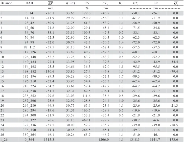
Actual Evapotranspiration (ER)
Data on ER’, s(ER’), CV, ET0, KC, ETC, the
evapotranspiration corrected by drainage ER, and QL,
are presented in Table 3. Water balances 5 to 22 were
chosen to estimate KC through the relation ER/ET0.
During these balances, soil water storage SL was high
Table 1 - Rainfall at the five replicates, average (P), standard deviations [s(P)], coefficients of variation (CV), and rainfall at the automatic meteorological station (Ps) of each period (DAB = days after beginning).
e c n a l a
B Period DAB Rainfalll( P)
1 2 3 4 5 s(P) CV Ps
-m m
-- % mm
1 09/01to09/15 0_14 4.0 4.2 4.3 4.2 4.0 4.1 0.1 3.2 5.2 2 09/15to09/29 14_28 5.8 5.8 6.4 4.8 6.2 5.8 0.6 10.6 1.2 3 09/29to10/13 28_42 79.0 75.4 80.6 78.0 75.9 77.8 2.2 2.8 84.2 4 10/13to 10/27 42_56 18.2 18.1 18.2 17.6 17.5 17.9 0.3 1.9 1.9 5 10/27to 11/10 56_70 25.4 24.9 26.3 24.5 25.5 25.3 0.7 2.7 46.5 6 11/10 to11/24 70_84 75.7 74.2 78.7 74.2 72.5 75.1 2.3 3.1 83.0 7 11/24 to12/08 84_98 93.9 88.9 91.8 87.4 86.7 89.7 3.0 3.4 90.6 8 12/08to 12/22 98_112 51.0 49.8 49.3 48.5 48.0 49.3 1.2 2.4 49.4 9 12/22to 01/05 112_126 89.2 86.5 85.1 84.4 82.8 85.6 2.4 2.8 89.8
0
1 01/05to01/19 126_140 52.4 51.1 50.5 49.6 49.3 50.6 1.2 2.5 52.7 1
1 01/19to02/02 140_154 173.7 168.4 165.7 166.7 164.2 167.7 3.7 2.2 170.7 2
1 02/02to02/16 154_168 73.9 71.4 69.1 67.9 66.9 69.8 2.8 4.0 69.4 3
1 02/16to03/01 168_182 156.6 156.3 153.7 149.2 148.8 152.9 3.7 2.5 143.4 4
1 03/01to03/15 182_196 75.9 74.8 72.2 71.4 71.2 73.1 2.1 2.9 74.8 5
1 03/15to03/29 196_210 14.4 14.4 14.0 13.8 13.2 14.0 0.5 3.6 15.0 6
1 03/29to04/12 210_224 59.4 78.6 62.2 65.0 61.0 65.2 7.7 11.9 46.6 7
1 04/12to04/26 224_238 54.7 53.6 51.8 50.9 50.7 52.3 1.7 3.3 56.8 8
1 04/26to05/10 238_252 23.9 24.1 22.9 22.3 22.7 23.2 0.8 3.4 28.7 9
1 05/10to05/24 252_266 27.4 27.2 25.1 23.9 24.1 25.5 1.7 6.5 28.8 0
2 05/24to06/07 266_280 105.5 104.5 101.1 98.5 97.7 101.5 3.5 3.4 103.2 1
2 06/07to06/21 280_294 7.6 8.0 7.1 6.7 6.5 7.2 0.6 8.7 10.0 2
2 06/21to07/05 294_308 2.4 2.0 1.8 1.6 1.6 1.9 0.3 17.8 2.2 3
2 07/05to07/19 308_322 33.2 33.1 32.5 32.2 32.3 32.7 0.5 1.4 43.6 4
2 07/19to08/02 322_336 46.8 45.4 43.9 43.6 43.1 44.6 1.5 3.4 44.9 5
2 08/02to08/16 336_350 0.0 0.0 0.0 0.0 0.0 0.0 0.0 0.0 0.3 6
2 08/16to08/30 350_364 0.0 0.0 0.0 0.0 0.0 0.0 0.0 0.0 0.0 m
u
S 09/01to08/30 0_364 1350.0 1340.7 1314.3 1286.9 1272.4 1312.9 33.4 2.5 1342.9 P
Table 2 - Irrigation at the five replicates, average (I), standard deviations s(I), and coefficients of variation (CV). (DAB = days after beginning).
e c n a l a
B Period DAB Irrigation(mm)
1 2 3 4 5 s(I) CV
-m m -- %
1 09/01 a09/15 0_14 46.2 30.9 47.4 22.6 23.7 34.2 12.0 35.1
6
enough to elicit assuming that plants had no restric-tion to soil water, and that differences between ER
and ET0 resulted from differences in plant
architec-ture and percent of crop cover. Exception has to be made to balances 11, 13 and 20, during which drain-age QL occurred. The variability of KC is large, rang-ing from 0.6 to 1.7, with an average of 1.1, standard
deviation 0.3, and CV=31.2%. To complete the KC
column on Table 3, the average KC was considered
for the water balances under water deficit and with drainage.
The highest ER value (6.8 mm day-1) was
ob-tained in balance 12, a coherent value for February in the region. The lowest values (0.9, 0.5, and 0.8 mm day-1, respectively) occurred on balances 2, 23, and 25. During these periods, coffee plants were under water deficit and, consequently, losing leaves.
Table 4 presents the calculation of the standard deviation s(ER') of the actual evapotranspiration,
cal-culated through error propagation since this component was obtained as an unknown in equation (2). From this table it can be seen that the greatest contribution to
comes from SLmeasurements. Although their CVs are
relatively low (Table 5), the magnitudes of the
stan-dard deviations of SL are much greater in relation to
those of the other components, giving a large
contri-bution to . The use of ∆S
L, which has a much lower
magnitude, does not improve the calculations since s(∆S
L) involves s(SLi) and s(SLf). As a result s(ER') is
very large in relation to its average ER’, indicated by the high CVs presented in Table 3. They varied from 27.4% to 469.1%, showing a great uncertainty in mea-suring actual evapotranspiration from water balances. Most of the high CVs correspond to wet periods, when ER was close to ETc, periods during which aerody-namic models like the combined methods of Penman, Slatyer & McIlroy, and Penman-Monteith (Pereira et al., 1997), yield much better estimatives. Therefore, it Table 3 - Average actual evapotranspiration (ER'), its standard deviation [s(ER’) calculated through equation 03], reference evapotranspiration (ET0), crop coefficient (KC), potential evapotranspiration (ETC), ER and the drainage below root zone (QL) for each period. (DAB = days after beginning).
e c n a l a
B DAB s(ER') CV ET
0 KC ETc ER
m
m % mm --- mm--- -1 0_14 -26.1 33.65 129.0 -45.9 1.1 -50.1 -26.1 0.0 2 14_28 -11.9 29.92 250.9 -56.0 1.1 -61.2 -11.9 0.0 3 28_42 -50.9 31.25 61.3 -53.9 1.1 -58.9 -50.9 0.0 4 42_56 -24.8 32.00 129.1 -65.4 1.1 -71.5 -24.8 0.0 5 56_70 -33.1 33.19 100.3 -47.5 0.7 -33.1 -33.1 0.0 6 70_84 -62.3 32.90 52.8 -60.3 1.0 -62.3 -62.3 0.0 7 84_98 -72.0 30.74 42.7 -50.5 1.4 -72.0 -72.0 0.0 8 98_112 -57.5 31.10 54.1 -62.4 0.9 -57.5 -57.5 0.0 9 112_126 -68.1 33.87 49.7 -57.5 1.2 -68.1 -68.1 0.0
0
1 126_140 -52.2 33.28 63.7 -63.2 0.8 -52.2 -52.2 0.0 1
1 140_154 -97.4 33.95 34.9 -39.3 1.1 -42.9 -42.9 -54.4 2
1 154_168 -95.5 34.66 36.3 -62.0 1.5 -95.5 -95.5 0.0 3
1 168_182 -130.6 35.80 27.4 -46.8 1.1 -51.2 -51.2 -79.4 4
1 182_196 -89.3 36.28 40.6 -52.3 1.7 -89.3 -89.3 0.0 5
1 196_210 -62.4 33.95 54.4 -55.3 1.1 -62.4 -62.4 0.0 6
1 210_224 -64.2 33.61 52.4 -47.7 1.3 -64.2 -64.2 0.0 7
1 224_238 -51.7 32.31 62.5 -36.1 1.4 -51.7 -51.7 0.0 8
1 238_252 -29.6 33.03 111.6 -35.6 0.8 -29.6 -29.6 0.0 9
1 252_266 -25.6 32.92 128.8 -24.4 1.0 -25.6 -25.6 0.0 0
2 266_280 -46.8 30.75 65.6 -23.4 1.1 -25.6 -25.6 -21.3 1
2 280_294 -19.6 31.51 160.5 -29.9 0.7 -19.6 -19.6 0.0 2
2 294_308 -21.9 33.59 153.2 -35.4 0.6 -21.9 -21.9 0.0 3
2 308_322 -6.6 31.13 469.1 -27.7 1.1 -30.2 -6.6 0.0 4
2 322_336 -57.5 30.00 52.2 -35.7 1.1 -39.0 -39.0 -18.5 5
2 336_350 -11.4 30.48 266.5 -45.1 1.1 -49.3 -11.4 0.0 6
2 350_364 -46.1 30.26 65.7 -46.7 1.1 -51.0 -46.1 0.0 6
2 _
1 0_364 -1315.3 - - -1206.0 1.1 -1318.3 -1141.7 -173.6 '
is not recommended to estimate ER through water bal-ances. That does not low the value of water balance techniques, since they are useful in many water man-agement practices, since they reflect in space and time, the water availability to the crop.
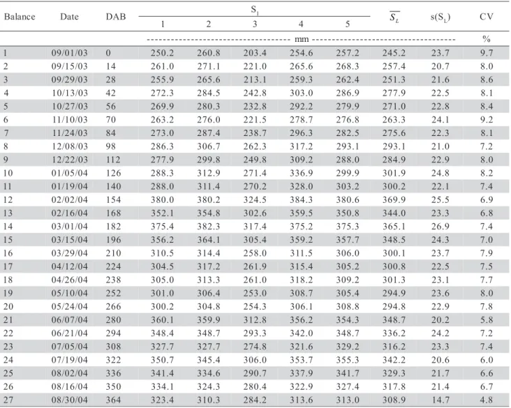
Soil Water Storage SL(ti)
Variability of the soil water storage (SL) cal-culated through the trapezoidal rule (equation 4) from
soil water content (θ) data collected by the neutron
probe is shown in Table 5. The CVs are relatively low and very consistent. Since three access tubes were placed in each plot, each average SL is the result of
15 measurements, what should be a good estimative of the soil water situation at the moment ti. Advantage of neutron probes over classical methodologies is that they allow measurements along time at exactly the same position. This explains the homogeneity of the CVs. The variability of the data shown in Table 5 de-picts accurately soil water variability of the experimen-tal field. Using the conventional methods, such as gauge sampling, it would not be possible to measure
θ always at the same positions, and this would
exceed-ingly increase data variability and would require a much larger experimental area, once samplings are de-structive.
The lowest value of SLmin (245.2 mm) was
reg-istered in Sep.01.2003, corresponding to a severe wa-ter stress condition, but still not high enough to stop crop growing. This value could be taken as a “field wilting point” in order to calculate a practical value of the available water holding capacity of the 0-1.0 m layer. For the field capacity one could take the value
of SLmax for Mar.01.2004, measured after a long
rain-fall period and with no subsequent deep drainage (Table 7). Considering these extreme values, the avail-able water capacity of this soil profile (SLmax-SLmin) is 120 mm, which represents the maximum possible variation of SL in this crop down to the depth of 1.0 m for this particular soil.
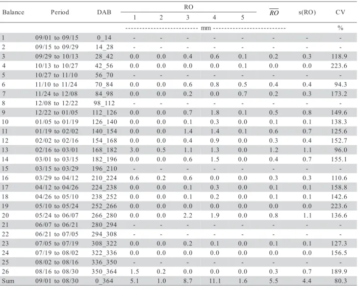
Runoff (RO)
The runoff was very small in relation to the other components (1.7% in relation to rainfall), pre-sented large variability, not appearing in all plots and in an inconsistent way. This means that the coffee Table 4 - Estimation of the standard deviation s(ER’) of the actual evapotranspiration ER’, using error propagation (equation
03), all in mm. (DAB = days after beginning).
e c n a l a
B DAB s(P) s(I) s(SLf) s(SLi) s(RO) s(ER') 1 0_14 0.1 12.0 20.7 23.7 0.0 33.6 2 14_28 0.6 0.0 21.6 20.7 0.0 29.9 3 28_42 2.2 0.0 22.5 21.6 0.3 31.2 4 42_56 0.3 0.0 22.8 22.5 0.0 32.0 5 56_70 0.7 0.0 24.1 22.8 0.0 33.2 6 70_84 2.3 0.0 22.3 24.1 0.4 32.9 7 84_98 3.0 0.0 21.0 22.3 0.3 30.7 8 98_112 1.2 0.0 22.9 21.0 0.0 31.1 9 112_126 2.4 0.0 24.8 22.9 0.8 33.9
0
1 126_140 1.2 0.0 22.1 24.8 0.1 33.3 1
1 140_154 3.7 0.0 25.5 22.1 0.7 33.9 2
1 154_168 2.8 0.0 23.3 25.5 0.4 34.7 3
1 168_182 3.7 0.0 26.9 23.3 1.1 35.8 4
1 182_196 2.1 0.0 24.3 26.9 0.7 36.3 5
1 196_210 0.5 0.0 23.7 24.3 0.0 34.0 6
1 210_224 7.7 0.0 22.5 23.7 0.3 33.6 7
1 224_238 1.7 0.0 23.1 22.5 0.1 32.3 8
1 238_252 0.8 0.0 23.6 23.1 0.1 33.0 9
1 252_266 1.7 0.0 22.9 23.6 0.0 32.9 0
2 266_280 3.5 0.0 20.2 22.9 1.1 30.7 1
2 280_294 0.6 0.0 24.2 20.2 0.0 31.5 2
2 294_308 0.3 0.0 23.3 24.2 0.0 33.6 3
2 308_322 0.5 0.0 20.6 23.3 0.1 31.1 4
2 322_336 1.5 0.0 21.7 20.6 0.0 30.0 5
2 336_350 0.0 0.0 21.4 21.7 0.0 30.5 6
crop planted on a 10% slope along contour-lines was adequate for runoff and, consequently, erosion con-trol.
The high CVs presented in Table 6 demand careful analysis. The presence of many null values may indicate that this variable probably does not follow the normal distribution and with very low mean values, CVs tend to increase by definition, even when the vari-able is correctly measured. Anyway, the absolute val-ues of RO were very small and affected very little the establishment of water balances.
Water Balances
Table 7 summarizes all water balance compo-nents.
The historic average of annual rainfall in Piracicaba is 1,257 mm, which shows that the con-sidered year (Sept.2003/Sept.2004) was slightly more rainy than normal. The irrigation in this region is not necessary for most perennial crops, coffee included.
The amount of irrigation water applied (71.6 mm) aimed solely to prevent blooming damage during wa-ter stress periods. When wawa-ter inputs (P+I) is consid-ered, RO represents only 0.4% of the balance, that is, this component was not significant under the con-ditions in which the evaluations were carried out. There was a tendency of increasing RO with increas-ing P. This fact is expected, but is very hard to be forecasted once RO depends more on rain inten-sity than on total amount of water. Since the analyzed period did not deviate significantly from the ordinary local rainfall intensities, it is expected that the adopted crop management procedures limit this component to minimum values, e.g. those shown in Table 6.
The drainage below the depth z =1.0 m was 12.5% of the balance, which can be more significant in wetter years. In terms of N leaching, a reflex of drainage, splitting the plots’ fertilization was adequate Table 5 - Initial soil water storage SL(ti) at each of the five replicates, average (SL), standard deviations s(SL), and coefficients
of variation (CV) of each period. (DAB = days after beginning).
e c n a l a
B Date DAB SI
S (
s L) CV
1 2 3 4 5
-m m
-- %
1 09/01/03 0 250.2 260.8 203.4 254.6 257.2 245.2 23.7 9.7 2 09/15/03 14 261.0 271.1 221.0 265.6 268.3 257.4 20.7 8.0 3 09/29/03 28 255.9 265.6 213.1 259.3 262.4 251.3 21.6 8.6 4 10/13/03 42 272.3 284.5 242.8 303.0 286.9 277.9 22.5 8.1 5 10/27/03 56 269.9 280.3 232.8 292.2 279.9 271.0 22.8 8.4 6 11/10/03 70 263.2 276.0 221.5 278.7 276.8 263.3 24.1 9.2 7 11/24/03 84 273.0 287.4 238.7 296.3 282.5 275.6 22.3 8.1 8 12/08/03 98 286.3 306.7 262.3 317.2 293.1 293.1 21.0 7.2 9 12/22/03 112 277.9 299.8 249.8 309.2 288.0 284.9 22.9 8.0
0
1 01/05/04 126 288.3 312.9 271.4 336.9 299.9 301.9 24.8 8.2 1
1 01/19/04 140 288.0 311.4 270.2 328.0 303.2 300.2 22.1 7.4 2
1 02/02/04 154 380.0 380.2 324.5 384.3 380.6 369.9 25.5 6.9 3
1 02/16/04 168 352.1 354.8 302.6 359.5 350.8 344.0 23.3 6.8 4
1 03/01/04 182 375.4 382.3 317.4 375.2 375.3 365.1 26.9 7.4 5
1 03/15/04 196 356.2 364.1 305.4 359.2 357.7 348.5 24.3 7.0 6
1 03/29/04 210 310.5 314.4 258.0 311.5 306.0 300.1 23.7 7.9 7
1 04/12/04 224 304.5 317.2 261.9 315.4 305.2 300.8 22.5 7.5 8
1 04/26/04 238 305.0 313.3 261.0 318.2 309.2 301.3 23.1 7.7 9
1 05/10/04 252 301.0 306.4 253.0 308.7 305.4 294.9 23.6 8.0 0
2 05/24/04 266 300.2 304.8 254.3 306.1 308.8 294.8 22.9 7.8 1
2 06/07/04 280 360.1 359.9 312.8 356.2 354.3 348.7 20.2 5.8 2
2 06/21/04 294 348.4 348.7 293.3 342.0 348.7 336.2 24.2 7.2 3
2 07/05/04 308 327.7 327.7 274.8 321.6 329.2 316.2 23.3 7.4 4
2 07/19/04 322 350.7 345.4 306.0 353.7 355.3 342.2 20.6 6.0 5
2 08/02/04 336 341.4 334.6 290.7 337.9 341.7 329.3 21.7 6.6 6
2 08/16/04 350 334.1 324.3 280.4 322.9 327.4 317.8 21.4 6.7 7
2 08/30/04 364 323.4 310.3 284.2 313.6 313.0 308.9 14.7 4.8
L
in relation to the water balance components. As the annual variation of ∆S
L should, theoretically, be small
along extended periods (e.g. one year or-5.5 mm in this case), the remaining of the water balance is ER, and represents 82.5%. In ideal situation, in which RO and
QL are null, ER would represent 100% of (P+I), that
is, ER = (P+I). Such condition almost happened over the studied year.
Figure 2 shows the distribution of rainfall and evapotranspiration along the year (Sept.2003/ Sept.2004). In general, the rainfall was well distributed, except for the unusual high rainfall rate during June and July (balances 20 to 24), ordinarily the driest months in the region. This exception guaranteed a good crop development. At the end of the dry season, rep-resented by balances 1 and 2; 25 and 26, irrigation was necessary. The highest rainfall occurred during bal-ances 11 and 13, and, as a consequence, the drainage (QL) was 12.5% of (P+I).
Table 6 - Runoff (RO) at each of the five replicates, average (RO), standard deviations (SD), and coefficients of variation (CV) from each period. (DAB = days after beginning).
e c n a l a
B Period DAB RO s(RO) CV
1 2 3 4 5
-m m
-- %
1 09/01to09/15 0_14 - - -
-2 09/15to09/29 14_28 - - -
-3 09/29to10/13 28_42 0.0 0.0 0.4 0.6 0.1 0.2 0.3 118.9 4 10/13to10/27 42_56 0.0 0.0 0.0 0.0 0.1 0.0 0.0 223.6
5 10/27to11/10 56_70 - - -
-6 11/10to11/24 70_84 0.0 0.0 0.6 0.8 0.5 0.4 0.4 94.3 7 11/24to12/08 84_98 0.0 0.0 0.2 0.0 0.7 0.2 0.3 173.2 8 12/08to12/22 98_112 - - - -9 12/22to01/05 112_126 0.0 0.0 0.7 1.8 0.1 0.5 0.8 149.6
0
1 01/05to01/19 126_140 0.0 0.0 0.1 0.3 0.0 0.1 0.1 138.3 1
1 01/19 to02/02 140_154 0.0 0.0 1.4 1.4 0.1 0.6 0.7 125.6 2
1 02/02to02/16 154_168 0.0 0.0 0.4 0.9 0.0 0.3 0.4 152.7 3
1 02/16to03/01 168_182 3.0 0.5 1.1 1.3 0.0 1.2 1.1 96.0 4
1 03/01to03/15 182_196 0.0 0.0 0.6 1.5 0.0 0.4 0.7 155.1 5
1 03/15to03/29 196_210 - - - -6
1 03/29to04/12 210_224 0.6 0.2 0.6 0.0 0.0 0.3 0.3 110.6 7
1 04/12to04/26 224_238 0.0 0.0 0.1 0.3 0.0 0.1 0.1 158.8 8
1 04/26to05/10 238_252 0.0 0.0 0.1 0.2 0.0 0.1 0.1 142.6 9
1 05/10to05/24 252_266 0.0 0.0 0.0 0.0 0.0 0.0 0.0 223.6 0
2 05/24to06/07 266_280 0.0 0.0 2.2 1.9 0.0 0.8 1.1 136.6 1
2 06/07to06/21 280_294 - - - -2
2 06/21to07/05 294_308 - - - -3
2 07/05to07/19 308_322 0.0 0.0 0.2 0.1 0.0 0.1 0.1 127.3 4
2 07/19to08/02 322_336 0.0 0.0 0.0 0.0 0.0 0.0 0.0 156.5 5
2 08/02to08/16 336_350 - - - -6
2 08/16to08/30 350_364 1.5 0.2 0.0 0.0 0.0 0.3 0.7 189.9 m
u
S 09/01to08/30 0_364 5.1 1.0 8.7 11.1 1.6 5.5 4.4 80.3 RO
The actual evapotranspiration got closer to the maximum almost along the whole year, except for the dry periods (balances 1, 2, 4, 23, 25, and 26). During these periods, the coffee plants lost part of their leaves because the soil hydraulic conductivity was too low, limiting water flux to the plant root system which did not attend atmospheric demand.
CONCLUDING REMARKS
In areas with neighboring obstacles, the dy-namics of the wind and, consequently, of the rainfall can be affected, and so measurement of the rainfall should be made with an adequate number of replicates. However, the use of data obtained at neighboring me-teorological station is not recommended. In this study, an area of 0.2 ha, with trees, silo, and warehouse be-tween 5 and 20 m high, and located within 100 m, five rain-gauges apart from each other 15 to 100 m,
pre-sented CVs ranging on 1.4 to 17.8%. The atmospheric demand of the coffee crop, expressed by its actual evapotranspiration, was 1141.7 mm per year, and was almost completely satisfied by rainfall input. In com-plex terrain, the water balance terms can display sub-stantial variability. To infer a representative estimate of the actual evapotranspiration as a remainder of the water balance, knowledge of the spatial variability of the other components is therefore necessary. Because of error propagation, estimates derived from a exceed-ingly small set of point measurements can be substan-tially flawed. For the agricultural year under analysis, the soil in question presented a maximum water hold-ing capacity of 120 mm, which represents a backup of water for 24 days considering an average demand of
5 mm day-1
, without considering the restrictions on water flux to the roots in drier periods. In this year, the rainfall was near to the long term average, and was enough to meet the atmospheric demand of the crop, Table 7 - Average values of rainfall (P), irrigation (I), soil water storage changes (ΔS), runoff (RO), drainage (QL),
actual evapotranspiration (ER), and potential evapotranspiration (ETC ), for all analyzed periods. (DAB = days
after beginning).
e c n a l a
B Period DAB
-m m
-1 09/01 to09/15 0_14 4.1 34.2 245.2 12.2 0.0 0.0 -26.1 -50.1 2 09/15 to09/29 14_28 5.8 0.0 257.4 -6.1 0.0 0.0 -11.9 -61.2 3 09/29 to10/13 28_42 77.8 0.0 251.3 26.6 -0.2 0.0 -50.9 -58.9 4 10/13to10/27 42_56 17.9 0.0 277.9 -6.9 0.0 0.0 -24.8 -71.5 5 10/27to 11/10 56_70 25.3 0.0 271.0 -7.8 0.0 0.0 -33.1 -33.1 6 11/10to11/24 70_84 75.1 0.0 263.3 12.3 -0.4 0.0 -62.3 -62.3 7 11/24 to12/08 84_98 89.7 0.0 275.6 17.5 -0.2 0.0 -72.0 -72.0 8 12/08to12/22 98_112 49.3 0.0 293.1 -8.2 0.0 0.0 -57.5 -57.5 9 12/22to01/05 112_126 85.6 0.0 284.9 17.0 -0.5 0.0 -68.1 -68.1
0
1 01/05 to01/19 126_140 50.6 0.0 301.9 -1.7 -0.1 0.0 -52.2 -52.2 1
1 01/19 to02/02 140_154 167.7 0.0 300.2 69.8 -0.6 -54.4 -42.9 -42.9 2
1 02/02 to02/16 154_168 69.8 0.0 369.9 -26.0 -0.3 0.0 -95.5 -95.5 3
1 02/16to03/01 168_182 152.9 0.0 344.0 21.1 -1.2 -79.4 -51.2 -51.2 4
1 03/01 to03/15 182_196 73.1 0.0 365.1 -16.6 -0.4 0.0 -89.3 -89.3 5
1 03/15 to03/29 196_210 14.0 0.0 348.5 -48.4 0.0 0.0 -62.4 -62.4 6
1 03/29 to04/12 210_224 65.2 0.0 300.1 0.7 -0.3 0.0 -64.2 -64.2 7
1 04/12 to04/26 224_238 52.3 0.0 300.8 0.5 -0.1 0.0 -51.7 -51.7 8
1 04/26 to05/10 238_252 23.2 0.0 301.3 -6.4 -0.1 0.0 -29.6 -29.6 9
1 05/10 to05/24 252_266 25.5 0.0 294.9 -0.1 0.0 0.0 -25.6 -25.6 0
2 05/24 to06/07 266_280 101.5 0.0 294.8 53.8 -0.8 -21.3 -25.6 -25.6 1
2 06/07to06/21 280_294 7.2 0.0 348.7 -12.4 0.0 0.0 -19.6 -19.6 2
2 06/21 to07/05 294_308 1.9 0.0 336.2 -20.0 0.0 0.0 -21.9 -21.9 3
2 07/05 to07/19 308_322 32.7 0.0 316.2 26.0 -0.1 0.0 -6.6 -30.2 4
2 07/19 to08/02 322_336 44.6 0.0 342.2 -12.9 0.0 -18.5 -39.0 -39.0 5
2 08/02 to08/16 336_350 0.0 0.0 329.3 -11.4 0.0 0.0 -11.4 -49.3 6
2 08/16 to08/30 350_364 0.0 37.5 317.8 -8.9 -0.4 0.0 -46.1 -51.0 m
u
S 09/01 to08/30 0_364 1312.8 71.6 7931.6 63.7 -5.5 -173.6 -1141.7 -1336.1
with restrictions in the period of dry and cold winter, favorable for blossoming. Soils with smaller storage capacity are likely to cause water supply problems and also permit larger values of internal drainage and, con-sequently, leaching. Soil water storage, although mea-sured carefully, was the component that introduced most variability and error propagation in water balance calculations. Coffee plantations in steep-sloped areas have to be made in a way that elicits good water infil-tration, minimizing runoff losses and erosion process. Planting made in furrows along contour-lines reduced considerably the runoff and so erosion neared zero. In this study, carried upon a soil with average slope 10%, the value runoff did not exceed 1.7% of total rainfall.
ACKNOWLEDGMENT
The authors thank FAPESP, CNPq and CAPES for finantial support and fellowships.
REFERENCES
BASANTA, M.del V. Dinâmica do nitrogênio na cultura de cana-de-açúcar em diferentes sistemas de manejo de resíduos da colheita. Piracicaba: USP/ESALQ, 2004. (Tese – Doutorado).
EMPRESA BRASILEIRA DE PESQUISA AGROPECUÁRIA. Centro Nacional de Pesquisa de Solo. Sistema brasileiro de classificação de solos. Rio de Janeiro: Embrapa Solos, 1999. 412p.
FNP CONSULTORIA & COMÉRCIO. Agrianual 2004: Anuário da Agricultura Brasileira. São Paulo, 2004. 185p.
GREGORICH, E.G.; CARTER, M.R. Soil qualify for crop production and ecosystem health. Amsterdam: Elsevier, 1997. 456p. MONTEITH, J.L. Principles of environmental physics. Elsevier: New
York, 1973. 241p.
PEREIRA, A.R.; VILLA NOVA, N.A.; SEDIYAMA, G.C.
Evapo(transpi)ração. Piracicaba: FEALQ, 1997. 183p.
PEREIRA, A.R.; ANGELOCCI, L.R.; SENTELHAS, P.C.
Agrometeorologia, fundamentos e aplicações. Guaíba: Livraria e Editora Agropecuária, 2002. 478p.
REICHARDT, K.; ANGELOCCI, L.R.; BACCHI, O.O.S.; PILOTTO, J.E. Daily rainfall variability at a local scale (1,000 ha), in Piracicaba, SP, Brazil, and its implications on soil water recharge. Scientia Agricola, v.52, p.43-49, 1995.
VILLA NOVA, N.A. Dados agrometeorológicos do município de Piracicaba. Piracicaba: ESALQ/Departamento de Física e Meteorologia, 1989.
VILLAGRA, M.M.; BACCHI, O.O.S.; TUON, R.L.; REICHARDT, K. Difficulties of estimating evaporation from the water balance equation. Agricultural and Forest Meteorology, v.72, p.317-325, 1995.
![Table 1 - Rainfall at the five replicates, average ( P ), standard deviations [s(P)], coefficients of variation (CV), and rainfall at the automatic meteorological station (Ps) of each period (DAB = days after beginning).](https://thumb-eu.123doks.com/thumbv2/123dok_br/15862394.663084/4.918.87.818.356.933/rainfall-replicates-deviations-coefficients-variation-automatic-meteorological-beginning.webp)