www.atmos-chem-phys.net/9/7491/2009/ © Author(s) 2009. This work is distributed under the Creative Commons Attribution 3.0 License.
Chemistry
and Physics
Vehicular emission of volatile organic compounds (VOCs) from a
tunnel study in Hong Kong
K. F. Ho1,2, S. C. Lee1, W. K. Ho1, D. R. Blake3, Y. Cheng1, Y. S. Li1, S. S. H. Ho1,2, K. Fung4, P. K. K. Louie5, and D. Park6
1Department of Civil and Structural Engineering, Research Center for Environmental Technology and Management, The Hong Kong Polytechnic University, Hung Hom, Kowloon, Hong Kong, China
2SKLLQG, Institute of Earth Environment, Chinese Academy of Sciences, Xi’an, 710075, China 3Department of Chemistry, University of California, Irvine, USA
4AtmAA Inc., 23917 Craftsman Road, Calabasas, CA 91302, USA
5Hong Kong Environmental Protection Department, 47/F, Revenue Tower, 5 Gloucester Road, Wan Chai, Hong Kong, China 6Railroad Environment Research Department, Korea Railroad Research Institute, Gyeonggi-Do, Korea
Received: 23 April 2009 – Published in Atmos. Chem. Phys. Discuss.: 2 June 2009 Revised: 13 August 2009 – Accepted: 10 September 2009 – Published: 7 October 2009
Abstract. Vehicle emissions of volatile organic compounds (VOCs) were determined at the Shing Mun Tunnel, Hong Kong in summer and winter of 2003. One hundred and ten VOCs were quantified in this study. The average concentra-tion of the total measured VOCs at the inlet and outlet of the tunnel were 81 250 pptv and 117 850 pptv, respectively. Among the 110 compounds, ethene, ethyne and toluene were the most abundant species in the tunnel. The total measured VOC emission factors ranged from 67 mg veh−1km−1 to 148 mg veh−1km−1, with an average of 115 mg veh−1km−1. The five most abundant VOCs observed in the tunnel were, in decreasing order, ethene, toluene,n-butane, propane and
i-pentane. These five most abundant species contributed over 38% of the total measured VOCs emitted. The high propane andn-butane emissions were found to be associated with liq-uefied petroleum gas (LPG)-fueled taxis. Fair correlations were observed between marker species (ethene, i-pentane,
n-nonane, and benzene, toluene, ethylbenzene and xylenes – BTEX) with fractions of gasoline-fueled or diesel-fueled ve-hicles. Moreover, ethene, ethyne, and propene are the key species that were abundant in the tunnel but not in gaso-line vapors or LPG. The ozone formation potential from the VOCs in Hong Kong was evaluated by the maximum incre-ment reactivity (MIR). It was found to be 568 mg of ozone
Correspondence to:S. C. Lee (ceslee@polyu.edu.hk)
per vehicle per kilometer traveled. Among them, ethene, propene and toluene contribute most to the ozone-formation reactivity.
1 Introduction
Vehicular emissions are one of major sources of volatile or-ganic compounds (VOCs) in the urban areas throughout the Pearl River Delta Region in China. The VOCs (e.g. benzene and 1,3-butadiene) emitted from vehicles directly influence human health due to their toxicity as well as are precursors for the formation of ozone (O3) and other photo-oxidants in ambient air (Finlayson-Pitts and Pitts, 1986). VOCs also play an important role in the formation of ground-level O3 and photochemical oxidants associated with urban smog (Monod et al., 2001). Photochemical smog is now an everyday oc-currence in many urban areas throughout the world. Smog is a mixture of secondary pollutants such as O3, nitrogen diox-ide (NO2), nitric acid (HNO3), aldehydes and other organic compounds, formed from photochemical reactions between nitrogen oxides (NOx) and hydrocarbons.
and engine operating conditions (e.g. cruising, idling, and transient modes) (Kaiser et al., 1992; Heeb et al., 1999, 2000; Tsai et al., 2003). With the chassis dynamometer tests, oper-ating conditions and fuel compositions can be adjusted and controlled, thus it has ability to examine vehicular emissions under different driving or loading settings and to effectively evaluate exhaust control technologies (Ning et al., 2008). Moreover, it is an ideal tool to distinguish between exhaust and evaporative emissions at a well-regulating environment (Liu et al., 2008). The drawbacks of chassis dynamometer test are expensive and time consuming in set-up. In addition, it cannot reflect the emissions from a real world traffic en-vironment where a composite of different on-road vehicles are being operated. For these reasons, another approach of roadway tunnel measurement has been developed and ap-plied to determine vehicular emissions in the past decade (e.g. Pierson et al., 1990; Haszpra and Szilagyi, 1994; Gertler et al., 1996; Duffy and Nelson, 1996; Mugica et al., 1998; Stemmler et al., 2005; Chiang et al., 2007). It directly deter-mines vehicular emission profiles and rates at a complicated on-road condition which mixes with emissions from vehi-cle tailpipes, unconsumed gasoline, and vehivehi-cle evaporative emissions. The result obtained is thus more representative and accurate in estimation of emissions from a large num-ber of vehicles to the local urban areas (Lonneman et al., 1986). The roadway tunnel measurements have several as-sumptions and limitations, including no cold start emissions, bias in fleet distributions, resistance caused by tunnel walls, and speed limits inside the tunnels.
Many tunnel studies reported the emission factors of indi-vidual and total VOCs. Stemmler et al. (1995) measured the emissions of carbon monoxide (CO), sulfur dioxide (SO2), NOx, and 26 individual VOCs including alkanes and aro-matic hydrocarbon in Gubrist tunnel in Switzerland in 1993. The emission factors of the total hydrocarbons are 426.5 and 432.5 mg km−1 for all vehicles and light duty vehicles, re-spectively.
In 2002, they have done a monitoring at the same location and found that the emission factors of particular VOCs were sufficiently lower than the values obtained in 1993 (Stemm-ler et al., 2005). For instance, the emission factors of benzene and toluene decreased from 13.69 to 2.7 mg km−1and 26.27 to 6.4 mg km−1, respectively. The figures indicate that the ef-ficient technology of modern car fleets with respect to VOCs emissions. In Taiwan, research also reported that paraffins and aromatics are the main VOCs groups in the tunnel (Chi-ang et al., 2007). The emission factors of total non-methane hydrocarbon (NMHC) were 440–1500 mg km−1(Chiang et al., 2007; Haw et al., 2002; Hsu et al.,2001).
Hong Kong is a densely populated city. According to the Hong Kong Transportation Department, there were 532 872 licensed vehicles in December 2004. Several ambient studies have recently been completed indicating vehicular emissions are the most important source for VOCs in Hong Kong (Lee et al., 2001; Ho and Lee, 2002; Guo et al., 2004). Liquefied
petroleum gas (LPG), gasoline, and diesel are the main fu-els used by vehicles in Hong Kong. In 2004, gasoline fueled vehicles accounted for 70.4% of the total licensed vehicles, while diesel and LPG fueled vehicles accounted for 24.5% and 3.5%, respectively (Hong Kong Transport Department, 2004). Vehicular performance affects fuel consumption and emissions in part because it would affect the combustion ef-ficiency and evaporative emissions from the fuel system. On the contrary, Turrio-Baldassarri et al. (2004) reported that synthesis and application of different types of fuels, modi-fications of engine designs, and improving emission control and catalytic technologies cause variations in emissions.
In Pearl River Delta Region, only researches (e.g. Guo et al., 2007; Chan et al., 2006; Barletta et al., 2005; Ho et al., 2004; Lee et al., 2002) reported the urban levels of VOCs. To our best knowledge, there are only limited measurement-based VOC emission profiles available in Hong Kong. This is a pilot study to determine local VOC emission profiles from vehicular exhaust. Air samples were collected in the heavy usage tunnel during winter and summer in 2003. The project also developed a reliable monitoring program to determine the emission factors of VOCs. The emission factors were es-timated by measuring the concentration differences between the tunnel inlet and outlet, the traffic rates, and the tunnel ventilation flux during sampling periods. The in-depth un-derstanding provides important information for management of Hong Kong air quality.
2 Methodology
2.1 Sampling location – Shing Mun Tunnel
Entrance Direction of traveling vehicle
350 m 600 m 686 m Inlet sampling location North Bore
South Bore Exit
Outlet sampling location
Sh
atin
T
su
an
W
an
Fig. 1.Schematic diagram of the Shing Mun Tunnel.
by the two sensors installed on the top roof of the tunnel near the sampling stations.
2.2 Sampling and instruments
In total, 23 pairs of whole air samples were collected in the tunnel, including five and 18 in summer and winter of 2003, respectively. From the results of valid samples, no statistical differences in emission factors were shown between summer and winter. We have thus combined the samples into calcu-lation. The sampling times were chosen to cover a wide vari-ation of vehicle usages at different time periods. One pair of samples was collected simultaneously at the tunnel entrance and exit during each sampling. The inlet sampling station was located 686 m inside the entrance of the south bore of Shing Mun Tunnel and the outlet sampling station was lo-cated 350 m upwind of the exit (Fig. 1). Ambient volatile organic canister samplers (AVOCS) (Andersen Instruments Inc. Series 97-300, Smyrna, GA, USA) were used to collect whole air samples into pre-cleaned and pre-evacuated 2-L stainless steel canisters at a flow rate of 30 mL min−1for 1 h in winter and 2 h in summer respectively. The canisters were pressurized when sampling. The sampler was fixed on the ground level with an inlet at a height of∼1.5 m. The flow rates were checked in the field before and after each run using a calibrated flow meter. After sampling, the filled canisters were shipped to the laboratory of the University of Califor-nia, Irvine for chemical analysis within two weeks of being collected.
2.3 Traffic count analysis
Vehicular composition and volume were determined by man-ual counts at the entrance of the tunnel tube at 15-min in-tervals during the sampling periods. Video-recording was also taken for data validation and review purposes. The vehicle types were classified into three major categories, namely 1) LPG-fueled taxis, 2) gasoline-fueled vehicles (e.g. motorcycles, private cars), and 3) diesel-fueled vehi-cles (e.g. mini- and large buses, light and heavy-duty trucks). Traffic speed surveys were periodically conducted at Shing Mun Tunnel using the car chasing method. The instrumented
vehicle equipped with a Darwin microwave speed sensor was driven and the tachometer sensor recorded vehicle speed on a second-by-second basis. The age and mileage distribution of vehicles were not obtained in this study.
2.4 Chemical analyses
All canisters were shipped to the laboratory at the Univer-sity of California, Irvine (UCI) and analyzed for CO, carbon dioxide (CO2), methane (CH4), and NMHCs. CO and CO2 analyses were carried out using a hydrogen gas methanizer upstream of a HP 5890 gas chromatography (GC) equipped with a flame ionization detector (FID) and an 3 m molecular sieve column. CH4was also analyzed using an HP 5890 GC equipped with an FID. The samples were injected into an 1/8′′ stainless steel 0.9 m column packed with 80/100 mesh
Spherocarb.
The analytical system used to analyze NMHCs (i.e. satu-rated, unsatusatu-rated, aromatic, and halogenated hydrocarbons) involved the cryogenic pre-concentration of 1520±1 cm3 (STP) of air sample in a stainless steel tube filled with glass beads (1/8′′ diameter) and immersed in liquid nitro-gen (−196◦C). A mass flow controller with a maximum al-lowed flow of 500 mL min−1controlled the trapping process. The trace gases were revolatilized using a hot water bath and then reproducibly split into five streams directed to different column-detector combinations.
Table 1.The 1-hr average traffic composition of Shing Mun Tunnel in summer and winter in 2003.
LPG* Gasoline Diesel Total
Taxis subtotal Motorcycles Private subtotal Mini- Large LDT HDT subtotal
Cars Buses Buses
Summer 233±33 233±33 42±10 918±198 961±203 115±43 168±73 357±179 695±467 1336±653 2529±697 (%) 9.9±3.7 9.9±3.7 1.8±0.5 38.2±10.9 39.9±11 5.1±3.2 6.6±2.3 13.5±4.5 25.0±13.1 50.1±15
Winter 145±60 145±60 29±18 593±205 622±220 46±13 108±48 173±103 282±164 69±241 1375±428 (%) 10.7±2.9 10.7±2.9 2.0±0.9 43.6±8.8 45.6±9.2 3.4±0.7 7.9±2.5 12.2±5.2 20.2±9.7 43.7±10.4
∗LPG: liquefied petroleum gas; LDT: light-duty trucks; HDT: heavy-duty trucks
film thickness) and output to the FID. The fourth com-bination (“Restek1701/ECD”) was a RESTEK 1701 col-umn (60 m×0.25 mm i.d.×0.50µm film thickness) which was output to the ECD. The fifth combination (“DB5-Restek1701/ECD”) was a DB-5 (J&W; 30 m×0.25 mm i.d. ×1µm film thickness) column connected in series to a RESTEK 1701 column (5 m, 0.25 mm i.d. ×0.5µm film thickness) and output to the ECD. The DB5ms/MS, DB1/FID, PLOT-DB1/FID, Restek1701/ECD, and DB5-Restek1701/ECD combinations received 10.1, 15.1, 60.8, 7.2, and 6.8% of the sample flow, respectively. Additional analytical details are given by Blake et al. (2001) and Colman et al. (2001). The measurement precision, detection limits and accuracy vary by compound and are quantified for each species in Colman et al. (2001). Briefly, the detection limit is 5 ppbv for CO, 0.01–10 pptv for halogenated hydrocarbons, and 3 pptv for other NMHCs (CH4is always above its detec-tion limit). The accuracy of our measurements is 5% for CO, 1% for CH4, 2–20% for halogenated hydrocarbons, and 5% for other NMHCs. The measurement precision is 2 ppbv for CO, 2 ppbv for CH4, 1–5% for halogenated hydrocarbons, and ranges from 0.5–5% for other NMHCs.
2.5 Emission factor
The emission factors from tunnel measurements were cal-culated according to the method of Pierson (Pierson and Brachaczek, 1983; Pierson et al., 1996). The vehicular emis-sion factor is the mass of specific pollutants produced in units of mg/kilometer, which can be determined from
EFveh=
(Cout−Cin)AU t
N L (1)
where EFveh is the average vehicular emission factor in mg vehicle−1km−1traveled.CoutandCinrepresent the mass concentrations of specific pollutants at the exit and entrance in mg m−3. Ais the area of tunnel cross-section in m2,U
is the wind speed in m s−1, andtis the sampling duration (1 or 2 h in this study).N is the total traffic number during the sampling period.Lis the distance between the two monitor-ing stations in km. The VOC concentrations at the entrance
of the tunnel were subtracted from those in the tunnel. The difference was multiplied by the tunnel air flow to determine the mass emitted during the run. This value was divided by the total vehicle distance traveling during the run to obtain the fleet mean emission rate.
2.6 Photochemical reactivity
It is well known that VOCs are significant precursors of O3 formation (Guo et al., 2004). Individual compound has dif-ferent characteristic photochemical reactivity. In order to cal-culate the O3-forming potential of the vehicular emissions, the speciated emission factors for each vehicle type were multiplied by the maximum incremental reactivity (MIR) scale developed by Carter (1998). The MIR are in units of grams of O3 per gram of organic compound and therefore are simply multiplied by the emission factors (grams of or-ganic compound per vehicle-km driven), to yield reactivity-adjusted emission rates in units of O3per vehicle-km.
3 Results and discussion
3.1 Run description
The average number of vehicles traversed the tunnel per hour during this study was 1545, ranging from 786 to 2842. Ta-ble 1 shows the 1-h average traffic composition of Shing Mun Tunnel in summer and winter in 2003. On average, approx-imately 47% of the total vehicles were diesel-fueled, 43% were gasoline, and the remaining were LPG vehicles. Diesel-fueled vehicles represented the highest proportion (more than 60%) during 11:00–13:00 and 14:00–16:00. The traf-fic speed for every run did not vary signitraf-ficantly, with most speeds recorded within the range of 60 to 70 km h−1. The av-erage wind speed recorded in the tunnel during the sampling periods was about 4.7 m s−1.
3.2 Concentrations of VOCs
Tunnel. These include CO, CO2, carbonyl sulfide (OCS), carbon disulfide (CS2), CH4, 40 C2–C10saturated hydrocar-bons, 32 C2–C10 unsaturated hydrocarbons, 21 C6–C10 aro-matic hydrocarbons and 12 halogenated hydrocarbons.
The average concentrations and standard deviations of the VOCs and their classes at the inlet and outlet of tunnel are given in Table 2. The average concentrations of the total NMHC (sum of all of measured species except CO, CO2, CH4, OCS and CS2) at the inlet and outlet of the tunnel were 81 000 pptv and 112 000 pptv, respectively. Among the 105 compounds, ethene was the most abundant VOC and ethyne was the next most abundant species, followed by toluene. Interestingly, propane is the fourth most abundant gas at the tunnel inlet whilen-butane is the fourth most abundant species at the outlet. This is thought to be the result of emis-sions arising from LPG vehicles (see Sect. 3.3). It has been reported that concentrations of individual VOCs in tunnels were typically 10 times higher than those of the same species measured in fresh air at the ventilation intake (Kirchstetter et al., 1996) or outside the tunnel (Mugica et al., 1998). In this study, the individual VOCs in the tunnel were generally 5– 10 times higher than those in Hong Kong ambient air (Guo et al., 2007). Although OCS emissions make up only a small fraction of the total sulfur emitted into the atmosphere com-pared to SO2, its relative inertness in the troposphere, OCS is transported to the stratosphere where it is photodissociated and oxidized to SO2 and ultimately sulfate particles. An-thropogenic sources of OCS arise from the combustion of biomass and fossil fuel. Emission of OCS from vehicles is one of such example (Fried et al., 1992). The average con-centrations of OCS at the inlet and outlet of the tunnel were 970 pptv and 1200 pptv, respectively, which is higher than that of free troposphere (510 ppt) (Carroll, 1985) and similar to that in Beijing, China (1340 ppt) (Mu et al., 2002).
For both sampling locations, unsaturated hydrocarbons were the most abundant hydrocarbon group (inlet: 43%±6%; outlet: 44%±5%) in the samples collected in the tunnel, fol-lowed by saturated (inlet: 37%±6%; outlet: 36%±5%) and aromatic hydrocarbons (inlet: 16%±2%; outlet: 17%±2%). The weight percentages between the two locations showed no significant differences compared to their absolute concen-trations. This is likely due to the fact that both of the loca-tions were affected predominantly by vehicle exhaust.
Differences between concentrations measured at the tun-nel outlet and those measured at the same time at the tuntun-nel inlet are also shown in Table 2. The VOC composition in the tunnel air is influenced by ambient VOC concentrations. Therefore, the VOC composition obtained from the concen-tration difference between the two sites inside the tunnel bet-ter represents the VOC composition as compared to the re-sults obtained from only one site. When looking at the net concentration, the five most abundant VOCs emitted by vehi-cles at the tunnel were, in decreasing order, ethene ethyne,n -butane, toluene and propane. This implies that ethene has the highest emission rate in vehicle exhaust. Ethene emissions in
the tunnel contributed more than 20% of the total NMHC emissions (except CO, CO2, CH4, OCS, and CS2) during most of the measurement periods. And the five most abun-dant species contributed over 50% of the total NMHC emis-sions. Based on the net concentration, unsaturated hydro-carbons (48%) are the most abundant, followed by saturated hydrocarbons (34%), and aromatics hydrocarbons (17%).
3.3 VOC ratios
Using the ratio of a more reactive VOC to a less reactive VOC (photochemical lifetimes (or reactivities) against hy-droxyl radical (OH), a higher ratio indicates relatively little photochemical processing of the air mass and major impact from primary emissions. On the other hand, a lower ratio is reflective of more aged VOC mixes and thus presumably that the VOCs were emitted from more distant sources (Guo et al., 2007). Comparisons of the ratios can be used to esti-mate the relative ages of air parcels. In this study, the ratios of ethene/ethane andm,p-xylene/ethylbenzene were used for comparison (Nelson and Quigley, 1983; Smyth et al., 1999; So and Wang, 2004). The average value of ethene/ethane and
m,p-xylene/ethylbenzene in tunnel (1.42±0.36, 4.64±2.34, 2.61±0.30) are higher than the ratios measured at the nearby sampling location at Tsuen Wan (1.21±0.68, 1.65±0.47) and other urban/rural sites in Hong Kong (Guo et al., 2007).
Ethene and ethyne are typical tracers for combustion, and thus vehicle exhaust was the likely source of these two gases (Stoeckenius et al., 2006). Tsai et al. (2006) concluded that the ethyne/ethene ratios for Hong Kong, Macau, Guangzhou and Zhuhai were 0.53±0.03, 1.06±0.04, 1.26±0.04 and 1.01±0.21, respectively. And the ethene level in the Hong Kong roadside was a factor of two higher than ethyne, whereas ethene and ethyne were close in Guangzhou, Zhuhai and Macau. The average ethyne/ethene ratio in this study is 0.45±0.07 which is close to the previous roadside study in Hong Kong.
3.4 Correlation of VOCs
Table 2.Average concentrations of VOCs and their emission factors in summer and winter.
Concentrations (ppt) Emission Factor (mg veh−1km−1)
VOCs inlet outlet Outlet minus inlet mean range
CO2(ppmv) 580±50 710±80 130±30 310 000±81 000 180 000–480 000 CO (ppbv) 2800±720 4100±1000 1300±390 1900±380 1300–2600 CH4(ppmv) 1.91±0.1 1.92±0.1 0.01±0.01 7.2±4.8 0.0–17 OCS 970±300 1200±450 200±440 0.8±1.3 0.0–5.0
CS2 110±97 190±340 83±340 0.4±1.3 0.0–6.0
alkane
ethane 4400±1500 5500±1800 1100±550 1.7±0.6 0.0+2.5 propane 5800±2800 8200±4000 2400±1300 5.7±2.5 1.6–13
i-butane 3500±1800 5300±2600 1700±900 5.5±2.2 2.5–11
n-butane 5700±2500 8500±3700 2800±1300 8.7±3.1 3.9–17 2,2-dimethylbutane 98±36 130±49 28±45 0.2±0.2 0.0–0.6 2,3-dimethylbutane 140±64 200±85 61±46 0.3±0.2 0.0–0.7 2,2,3-trimethylbutane 8.0±4.0 12±4.0 3.0±2.0 0.0±0.0 0.0–00
i-pentane 3200±1100 4600±1600 1500±660 5.6±2.1 3.1–11
n-pentane 980±310 1400±480 450±210 1.7±0.6 0.9–3.3 2-methylpentane 940±330 1300±470 400±210 1.8±0.7 0.3–3.1 3-methylpentane 670±220 940±310 270±140 1.2±0.5 0.4–2.0 3-ethylpentane 55±100 53±23 −2±96 0.0±0.0 0.0–0.2 2,2-dimethylpentane 24±10 34±13 10±5.0 0.1±0.0 0.0–0.1 2,3-dimethylpentane 57±71 64±51 7.0±68 0.1±0.1 0.0–0.4 2,4-dimethylpentane 74±28 110±42 34±18 0.2±0.1 0.1–0.3 3,3-dimethylpentane 48±53 55±22 8.0±48 0.1±0.0 0.0–0.2 2,2,4-trimethylpentane 350±280 490±330 140±250 1.0±0.7 0.0–2.3 2,3,4-trimethylpentane 91±52 130±88 40±46 0.2±0.2 0.0–0.7
n-hexane 680±270 980±410 300±200 1.3±0.5 0.5–2.6 2-methylhexane 390±340 480±180 90±290 0.7±0.3 0.0–1.1 3-methylhexane 490±760 490±180 4±720 0.8±0.3 0.0–1.2 2,5-dimethylhexane 150±180 190±100 41±170 0.4±0.2 0.0–0.9 2,4-dimethylhexane 180±220 220±110 37±220 0.4±0.2 0.0–0.9 2,3-dimethylhexane 74±40 120±72 46±39 0.3±0.2 0.0–0.6
n-heptane 430±460 530±200 95±390 0.9±0.4 0.0–2.4 2-methylheptane 94±30 150±48 55±25 0.3±0.1 0.2–0.6 3-methylheptane 99±31 140±44 39±21 0.2±0.1 0.0–0.4 4-methylheptane 10±6.0 17±10 8.0±5.0 0.1±0.0 0.0–0.1 2,4-dimethylheptane 35±21 62±28 27±19 0.1±0.1 0.0–0.2 2,5-dimethylheptane 14±6.0 25±10 10±5.0 0.1±0.0 0.0–0.1 2,6-dimethylheptane 28±23 39±23 12±21 0.2±0.1 0.0–0.6 3,3-dimethylheptane 11±6.0 18±9.0 8.0±5.0 0.1±0.0 0.0–0.1 4,4-dimethylheptane 15±7.0 23±10 8.0±4.0 0.1±0.0 0.0–0.1
n-octane 150±54 230±76 84±36 0.5±0.2 0.1–0.9
n-nonane 140±77 240±107 96±54 0.7±0.4 0.3–1.6
n-decane 140±100 245±120 103±71 0.8±0.6 0.0–2.4 cycloalkane
cylopentane 530±210 810±340 290±150 1.0±0.4 0.6–1.7 methylcyclopentane 320±110 470±170 150±65 0.7±0.2 0.4–0.9 methylcyclohexane 220±170 280±110 62±130 0.4±0.2 0.0–0.8 cyclohexane 180±93 240±99 62±39 0.3±0.1 0.0–0.6 alkene
ethene 16000±4200 25000±7100 8500±3400 13±4.0 0.6–21 propene 4500±1100 6900±1900 2400±900 5.3±1.5 3.2-8.3
i-butene 1700±510 2600±850 840±560 2.5±1.3 0.0-4.7
cis-2-butene 290±99 450±160 160±62 0.5±0.1 0.3–0.8
trans-2-butene 400±130 620±210 220±87 0.6±0.2 0.5–1.1
1-butene 940±250 1500±380 530±210 1.6±0.6 0.4–2.6 1,3-butadiene 410±390 360±340 −46±360 0.3±0.6 0.0-2.3 2-methyl-1-butene 210±82 330±130 120±53 0.5±0.2 0.2–0.9 2-methyl-2-butene 260±180 400±240 140±130 0.6±0.4 0.0–1.7 3-methyl-1-butene 110±32 170±52 61±22 0.2±0.1 0.1–0.3
trans-2-pentene 270±100 440±170 160±71 0.6±0.2 0.3–1.0
Table 2.Continued.
Concentrations (ppt) Emission Factor (mg veh−1km−1)
VOCs inlet outlet Outlet minus inlet mean range
2-methyl-1-pentene 260±150 460±280 200±130 0.9±0.5 0.1–1.9
3-methyl-1-pentene 69±31 99±31 30±32 0.2±0.1 0.0–0.3
4-methyl-1-pentene 93±31 170±57 73±38 0.3±0.1 0.2–0.6
2-methyl-2-pentene 78±43 120±60 43±37 0.2±0.2 0.0–0.7 cis-3-methyl-2-pentene 67±37 100±51 38±31 0.2±0.1 0.0–0.6
trans-3-methyl-2-pentene 42±26 63±35 21±24 0.1±0.1 0.0–0.4
1-hexene 130±56 210±110 86±72 0.4±0.3 0.0–1.3
cis-2-hexene 44±17 74±29 30±14 0.1±0.0 0.1–0.2
trans-2-hexene 81±29 140±49 55±24 0.2±0.1 0.1–0.4
cis-3-hexene 21±6.0 27±10 6.0±12 0.0±0.0 0.0–0.1
trans-3-hexene 34±14 54±23 20±11 0.1±0.0 0.0–0.2
limonene 9.0±5.0 11±9.0 5.0±11 0.0±0.1 0.0–0.4
α−pinene 12±7.0 10±7.0 1.0±5.0 0.0±0.0 0.0–0.1
β-pinene 6.0±3.0 5.0±2.0 0.0±2.0 0.0±0.0 0.0–0.0
isoprene 160±340 56±63 −110±360 0.0±0.0 0.0–1.0
alkyne
ethyne 7400±1800 10000±2600 3000±1300 4.0±1.3 1.6–7.0
propyne 320±74 480±130 160±67 0.3±0.1 0.2–0.5
2-butyne 5.0±2.0 8.0±2.0 42±186 0.0±0.0 0.0–0.0
1-butyne 12±5.0 21±7.0 9.0±4.0 0.0±0.0 0.0–0.1
aromatic hydrocarbon
benzene 2500±620 3500±920 1100±380 4.5±0.9 2.5–6.0
ethylbenzene 590±210 820±270 240±110 1.3±0.4 0.7–2.0
1,4-diethylbenzene 69±56 150±72 84±75 0.6±0.4 0.0–1.3
1,3-diethylbenzene 31±15 53±22 25±27 0.2±0.2 0.0–0.6
1,2-diethylbenzene 17±9 25±13 10±11 0.1±0.1 0.0–0.3
1,2,3-trimethylbenzene 280±150 480±190 250±340 1.4±1.1 0.0–3.8 1,2,4-trimethylbenzene 720±400 1200±460 480±460 3.0±2.4 0.0–8.3 1,3,5-trimethylbenzene 180±70 300±92 120±72 0.8±0.4 0.3–1.8
isopropylbenzene 33±10 48±17 15±13 0.1±0.1 0.0–0.2
n-propylbenzene 120±41 200±63 74±43 0.5±0.2 0.2–0.9
isobutylbenzene 7.0±3.0 10±5.0 5.0±4.0 0.0±0.0 0.0–0.1
sec-butylbenzene 20±11 31±15 14±11 0.1±0.1 0.0–0.3
n-butylbenzene 23±10 35±16 15±19 0.1±0.1 0.0–0.4 toluene 6100±2000 8700±2800 2500±1200 12±3.9 6.9–23
2-ethyltoluene 210±99 380±140 170±140 1.0±0.7 0.0–2.5
3-ethyltoluene 320±130 530±200 210±180 1.4±0.9 0.0–3.7
4-ethyltoluene 130±61 270±230 130±210 0.7±0.8 0.0–2.8
isopropyltoluene 6.0±3.0 7.0±3.0 2.0±5.0 0.0±0.0 0.0–0.1
o-xylene 640±180 940±310 290±160 1.6±0.6 0.7–2.8
m-xylene 1000±320 1500±500 470±230 2.6±0.9 1.3–4.6
p-xylene 450±140 660±210 200±96 1.1±0.4 0.6–2.0
halogenated hydrocarbon
CH3Cl 800±140 790±140 −11±87 0.0±0.0 0.0–0.7
CH2Cl2 180±140 190±140 9.0±46 0.1±0.1 0.0–0.4
CHCl3 28±19 28±13 0.0±4.0 0.0±0.0 0.0–0.1
CCl4 99±4.0 100±3 0.0±3.0 0.0±0.0 0.0–0.1
CH3Br 50±120 72±190 22±78 0.1±0.5 0.0–2.3
CH2Br2 1.4±0.2 1.2±0.2 −0.1±0.1 0.0±0.0 0.0–0.0
CHBr3 4.2±2.1 4.6±1.9 0.4±1.2 0.0±0.0 0.0–0.1
CHCl3 28±19 28±13 0.0±4.0 0.0±0.0 0.0–0.1
1,2-dichloroethene 18±14 20±15 2.0±4.0 0.0±0.0 0.0–0.1
C2HCl3 50±78 51±81 2.0±9.0 0.0±0.0 0.0–0.2
C2Cl4 96±91 95±85 −1±13 0.0±0.0 0.0–0.2
H-1211 (CBrClF2) 7.0±4.0 8.0±5.0 0.0±1.0 0.0±0.0 0.0–0.1
saturateda 31 000±11 000 43000±15000 13 000±6400 23–66
unsaturatedb 35 000±8400 52 000±14 000 17 000±6400 35±9.4 16–56 aromatic hydrocarbon 13 000±3800 20 000±6100 6400±3200 33±11 18–50 halogenated hydrocarbon 1400±400 1400±380 26±130 0.5±0.5 0.0–2.4 total NMHCs 81 000±21 000 120 000±32 000 37 000±14 000 115±26 67–150
Table 3.Correlation of emission factors of selected VOCs with the change of the fractions of vehicle types.
VOCs Linear Regressiona R
LPG-fueled vehicles
propane propane=1.53+35.1χL 0.58
i-butane i-butane=1.87+32.2χL 0.55
n-butane n-butane=3.61+46.0χL 0.54
ethane ethane=1.15+6.50χL 0.54
gasoline-fueled vehicles
toluene toluene=2.78+23.00χg 0.68
ethylbenzene ethylbenzene=0.03+2.97χg 0.68
m-xylene m-xylene=0.137+5.58χg 0.62
3-methylpentane 3-methylpentane=0.21+2.55χg 0.62
i-butene i-butene=0.18+6.15χg 0.60
p-xylene p-xylene=0.235+2.02χg 0.57
o-xylene o-xylene=0.20+3.25χg 0.56
2-methylpentane 2-methylpentane=0.27+3.70χg 0.55
i-pentane i-pentane=1.06+11.3χg 0.53
n-pentane n-pentane=0.19+3.45χg 0.53
ethane ethane=0.87+2.22χg 0.52
3-ethyltoluene 3-ethyltoluene=0.26+3.77χg 0.45
1,2,3-triethylbenzene 1,2,4-trimethylbenzene=−0.83+5.47χg 0.45
n-hexane n-hexane=0.36+1.92χg 0.44
1,2,4-trimethylbenzene 1,2,4-trimethylbenzene=−0.78+8.81χg 0.40
diesel-fueled vehicles
ethene ethene=3.98+21.7χd 0.74
1-pentene 1-pentene=−3.28+12.0χd 0.59
1-butene 1-butene=0.48+2.58χd 0.53
propene propene=2.56+6.69χd 0.49
ethyne ethyne=2.36+4.47χd 0.46
benzene benzene=3.00+3.21χd 0.44
aχ
L=fractions of LPG-fueled vehicles;χg=fractions of gasoline-fueled vehicles;χd=fractions of diesel-fueled vehicles.
that the formation of isoprene from vehicular emission is un-certain. The variations of fuel types and vehicular engines used in different countries are possible explanation.
Moreover, strong and fair correlations were determined from marker species of fuel vapor (LPG, gasoline, and diesel). Propane, n-butane and i-butane are the major constituents of LPG in Hong Kong (Tsai et al., 2006) and strong correlations were found (R=0.95–0.98) among the species which indicated that unburned LPG was emit-ted to the tunnel atmosphere. n-pentane, i-pentane, 2,3-dimethylbutane, 2-methylpentane and toluene are the most abundant VOCs from the exhaust of gasoline-fueled vehi-cle and the evaporative loss from gasoline vapor (Tsai et al., 2006). Strong correlations (R=0.82–0.96) of these species indicated the importance of emissions from gasoline-fueled vehicles. Moreover, good correlations (R=0.54–0.95) were observed among diesel-fueled species (n-nonane, n-decane and 1,2,4-trimethylbenzene) (Tsai et al., 2006).
3.5 Emission factors of VOCs
The average emission factors of VOCs are given in Ta-ble 2. (Zero emission factors for some VOCs results from Coutlet begins less than or the same as Cinlet). The total measured VOC emission factors ranged from 67.2 mg veh−1km−1 to 148 mg veh−1km−1. The average emission factor was 115 mg veh−1km−1. The five most abundant VOC species in vehicle emissions were, in de-creasing order, ethene (12.6±4.3 mg veh−1km−1), toluene (12.1±3.9 mg veh−1km−1),n-butane (8.7
±3.1 mg veh−1 km−1), propane (5.7
Table 4.Emission factors of select VOC compounds for LPG, gasoline and diesel-fueled vehicles from regression of experimental data.
LPG gasoline diesel
VOCs Emission R Emission R Emission R
Factor Factor Factor
(mg veh−1km−1) (mg veh−1km−1) (mg veh−1km−1)
ethene −0.47 0.21±3.06 −0.71 25.7±2.62 0.74 toluene 0.30 25.7±3.56 0.68 2.89±2.84 −0.65
n-butane 49.6±15.1 0.54 0.32 3.89±2.41 −0.40 propane 36.6±10.1 0.58 0.38 1.50±1.63 −0.46
i-pentane 0.39 12.3±2.60 0.53 0.89±1.96 −0.54
i-butane 34.1±10.5 0.55 0.33 1.99±1.67 −0.41 propene −0.22 1.23±1.78 −0.51 9.34±1.66 0.49 benzene −0.17 2.21±1.03 −0.46 6.21±0.87 0.44 ethyne −0.34 1.67±1.32 −0.43 6.84±1.16 0.46 1,2,4-trimethylbenzene 0.35 8.03±2.65 0.40 −0.42
m-xylene 0.35 5.72±0.97 0.62 0.21±0.75 −0.60
i-butene 0.29 6.33±1.11 0.60 0.13±0.93 −0.58 1-pentene −0.31 −0.59 8.76±2.17 0.59 2-methylpentane 0.30 3.97±0.75 0.55 0.27±0.60 −0.53 ethane 7.65±2.14 0.54 3.08±0.49 0.52 0.69±0.38 −0.59
n-pentane 0.38 3.64±0.75 0.53 0.12±0.57 −0.55 1-butene −0.21 −0.57 3.06±0.53 0.53
o-xylene 0.39 3.46±0.68 0.56 0.21±0.51 −0.55 1,2,3-trimethylbenzene 0.28 4.64±1.59 0.45 −0.44 3-ethyltoluene 0.03 3.51±1.00 0.45 −0.39
n-hexane −0.03 2.28±0.52 0.44 −0.37 ethylbenzene 0.37 3.00±0.43 0.68 0.07±0.34 −0.66 3-methylpentane 0.38 2.76±0.44 0.62 0.17±0.36 −0.61
p-xylene 0.32 2.26±0.40 0.57 0.26±0.31 −0.55
OCS ranged from 0.05 to 3.2 mg veh−1km−1. The average emission factor was 0.8 mg veh−1km−1which is higher than previous study done by chassis dynamometer (Fried et al., 1992).
Linear regression analysis was carried out to determine the variations of emission factors of individual VOC with the change of the fractions of vehicle types (LPG-fueled taxis, gasoline-fueled vehicles, and diesel-fueled vehicles) in tunnel. The equations of linear regression and corre-lation coefficient of selected VOCs (total emission factor
>1 mg veh−1km−1 and R>0.4) are presented in Table 3. High propane,i-butane,n-butane and ethane emissions were found to be associated with a high proportion of LPG-fueled taxis. Fair correlations were observed between propane, i -butane,n-butane and ethane with the fractions of LPG-fueled taxis (R=0.54–0.58). Moreover, fair correlations were de-termined between marker species with fractions of gasoline-fueled and diesel-gasoline-fueled vehicles (Table 3).
The emissions of LPG-, gasoline-, and diesel-fueled vehi-cles can be differentiated from the regression equations of emissions of emission factors of individual VOC with the change of the fractions of vehicle types (under the conditions of total emission factor>1 mg vhe−1km−1 andR>±0.4).
The uncertainty estimate for the emission factor was deter-mined from the regression statistics. The emission factors of selected VOCs from Shing Mun Tunnel are presented in Table 4. The correlation coefficient (R) for the plot of the experimental emission factors was also shown. The three VOCs with the largest LPG-fueled emission factors were, in decreasing order,n-butane, propane, andi-butane. In addi-tion, the three most abundant VOCs in gasoline- and diesel-fueled vehicles emission were, in decreasing order, toluene, i-pentane, 1,2,4-trimethylbenzene, and ethane, propene, 1-pentene, respectively.
3.6 Effect of fuel evaporative loss in the tunnel atmosphere
Fig. 2.Average VOC distributions (presented in w/w%) for gasoline vapor, LPG and Shing Mun Tunnel samples.
pressures and thus do not quickly evaporate into the atmo-sphere (Tsai et al., 2006), suggesting that evaporative loss from diesel to the tunnel atmosphere was insignificant com-pared with the light species from gasoline and LPG. It is clear that there are several VOCs that were abundant in the tunnel but not the gasoline vapors or LPG samples, namely ethene, ethyne, and propene. These species are typical tracers for fossil fuel combustion.
Propane,i-butane andn-butane are tracers for LPG, the propane/(n-+i-butanes) ratio of LPG was 0.30, and the ra-tio of tunnel sample ranged from 0.24 to 0.51. The simi-lar propane/(n-+i-butanes) ratio obtained in Shing Mun Tun-nel and the LPG samples indicates that the propane and bu-tanes measured in the tunnel resulted from running evapo-rative losses of LPG. These findings are consistent with the previous study (Tsai et al., 2006). Moreover, the abundances of toluene and i-pentane were high in Shing Mun Tunnel. These two gases are tracers of gasoline evaporation (Tsai et al., 2006) The high concentrations observed in tunnel indi-cated the evaporative loss from gasoline-fueled vehicles is one of the sources for toluene andi-pentane. Gasoline evap-oration was found to contribute 14% of total VOC emission in Hong Kong in 2001–2002 (Guo et al., 2006).
3.7 Reactivity with respect to ozone formation
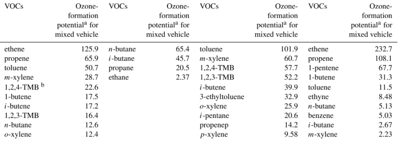
Table 5.Top 10 VOCs for ozone-forming potential of LPG, gasoline and diesel-fueled vehicles emissions estimated at Shing Mun Tunnel.
VOCs Ozone- VOCs Ozone- VOCs Ozone- VOCs Ozone-formation formation formation formation potentialafor potentialafor potentialafor potentialafor mixed vehicle mixed vehicle mixed vehicle mixed vehicle ethene 125.9 n-butane 65.4 toluene 101.9 ethene 232.7 propene 65.9 i-butane 45.7 m-xylene 60.7 propene 108.1 toluene 50.7 propane 20.5 1,2,4-TMB 57.7 1-pentene 67.7
m-xylene 28.7 ethane 2.37 1,2,3-TMB 52.2 1-butene 31.3 1,2,4-TMBb 22.6 i-butene 39.9 toluene 11.5 1-butene 17.5 3-ethyltoluene 32.9 ethyne 8.48
i-butene 17.2 o-xylene 25.9 n-butane 5.13 1,2,3-TMB 16.4 i-pentane 20.6 benzene 5.03
n-butane 12.6 propenep 14.2 i-butane 2.67
o-xylene 12.4 p-xylene 9.58 m-xylene 2.23
aOzone formation potential is calculated as emission factor of VOCs (mg veh−1km−1) multiplied by maximum incremental reactivity
(MIR) coefficient (dimensionless, gram of ozone produced per additional gram of VOCs).
bTMB represents trimethylbenzene.
VOCs is 115 mg veh−1km−1) which is similar to the results of Taipei tunnel, of 427 g (Hwa et al., 2002). Using the same calculation method, the top ten O3-forming potential of diesel-, LPG-, gasoline-fueled vehicles emission are de-termined. The largest contributors to O3production in Shing Mun Tunnel for LPG-, gasoline-, and diesel-fueled vehicles weren-butane, toluene, and ethene, respectively.
3.7.1 Comparison of tunnel results with other studies
Of studies that identified VOCs from vehicular emissions in tunnels, few have included calculations of emission fac-tors. A summary of literature data for selected VOCs are shown in Table 6. Generally, the emission factors from our study are similar or lower than other tunnel studies. The three largest abundant emission factors of VOCs in a Taipei Tunnel are toluene, ethene and 1,2,4-trimethylbenzene (29.0±4.95, 26.2±4.89 and 14.3±2.94 mg km−1veh−1, re-spectively), which are 2 to 5 times higher than our study (Hwa et al., 2002). Characteristic VOCs emissions may di-rectly reflect the specific formula of gasoline or diesel fuel used. The values of the benzene, toluene, and xylene (BTX) and i-pentane emission factors are about 20% lower than given in another tunnel studies as indicated in Table 6. This maybe due to the low fractions of gasoline-fueled vehicles in tunnels studied when compared to other studies. For propane andi-butane, the emission factors measured in our study are higher than previously measured in Taiwan and Switzerland. Due to the difference in fuel composition (i.e. 10% of LPG fueled vehicles) in Hong Kong, significantly higher emis-sion factors of propane and i-butane were anticipated and observed. This also demonstrates the need to establish local emission profiles.
4 Conclusions
Ethene, i-pentane and toluene were found to be the most abundant VOCs generated from the fueled vehicles. In this pilot vehicle source study, our observations are consistent with other studies done in Europe and Asian cities. But the average emission factor of OCS (0.8 mg veh−1km−1) was higher than previous study done by chassis dynamometer. These emission factors provide reliable estimations of VOCs introduced into the atmosphere from vehicular sources. On the basis of 100 g VOCs emitted, ozone formation is 494 g (average emission rate of total VOCs is 115 mg veh−1km−1) which is similar to the results of Taipei tunnel, of 427 g. This information will be useful in determining emission controls for different classes of vehicles. This will also allow for estimating the impact of VOC emissions from non mobile sources.
Acknowledgements. This project is supported by the study of De-termination of Suspended Particulate & VOC Emission Profiles for Vehicular Sources in Hong Kong (Tender Ref. AS 02-342) funded by Hong Kong Environment Protection Department (HKEPD), the Research Grants Council of Hong Kong (PolyU5204/07E), the Hundred Talents Program (Observation and modeling of secondary organic aerosol formation in China – KZCX2-YW-BR-10) of the Chinese Academy of Sciences.
The authors are grateful to Judith C. Chow and John G. Watson for their significant contributions to our sampling plan, and to HKEPD for provision of the data sets and permission for publication. The content of this paper does not necessarily reflect the views and policies of the HKSAR Government, nor does mention of trade names or commercial products constitute endorsement or recommendation of use.
Table 6.Comparison of emission factors of VOCs (mg veh−1km−1) with other studies.
This Study Hwa et al., Chiang et al., Staehelin et al. Staehelin et al. 2002 2007 1998 1998 Tunnel, Location Shing Mun Tai Pei Chung-Liao Gubrist Gubrist Tunnel, Hong Tunnel, Tunnel, Tunnel, Tunnel, Kong Taiwan Taiwan Switzerland Switzerland Year of Experiment 2003 2000 2005 1993 1993 Type of Vehicle LPG, gasoline, gasoline and gasoline and gasoline diesel
and diesel diesel diesel
ethene 13 26 – 24 45
toluene 12 29 29 16 21
n-butane 8.7 6.6 5.1 9.7 27
propane 5.7 2.4 0.2 0.15 5.7
i-pentane 5.6 13 40 18 43
i-butane 5.5 4.6 – 1.7 5.2
propene 5.3 12 10 14 22
benzene 4.5 12 5.9 10 15
ethyne 4.0 12 – 13 16
1,2,4-trimethylbenzene 3.0 14 12 4.6 9.6
m-xylene 2.6 9.0 8.4 11 27
p-xylene 1.1 –
i-butene 2.5 – – 8.0 11
1-pentene 1.9 1.6 0.97 0.61 3.4
2-methylpentane 1.8 5.3 13 – –
ethane 1.7 4.3 – 4.3 3.2
n-pentane 1.7 9.5 19 6.2 16
1-butene 1.6 8.3 11 1.9 5.0
o-xylene 1.6 7.9 6.4 4.8 6.3
1,2,3-trimethylbenzene 1.4 – 2.0 0.97 2.4
n-hexane 1.3 4.2 5.7 1.7 2.9
ethylbenzene 1.3 5.9 5.3 3.6 7.2
3-methylpentane 1.2 6.4 5.6 – –
2,2,4-trimethylpentane 1.0 0.29 0.77 – –
cylopentane 1.0 0.89 2.0 – –
n-heptane 0.9 1.5 1.6 0.93 2.3
n-decane 0.8 – 0.07 0.03 7.7
1,3,5-trimethylbenzene 0.8 2.3 3.7 1.5 2.7
3-methylhexane 0.8 2.9 2.8 – –
n-nonane 0.7 0.5 0.3 0.07 1.7
2-methylhexane 0.7 – 2.5 – –
trans-2-butene 0.6 1.6 0.81 1.4 2.9
n-octane 0.5 1.3 0.78 0.22 1.4
n-propylbenzene 0.5 1.7 1.7 0.68 1.9
cis-2-butene 0.5 1.8 1.6 1.3 2.5 1,3-butadiene 0.3 2.6 3.8 1.6 −1.6 2,3-dimethylbutane 0.3 1.3 13 – –
cyclohexane 0.3 0.98 0.4 4.5 6.1
References
Borbon, A., Fontaine, H., Veillerot, M., Locoge, N., Galloo, J. C., and Guillermo, R.: An investigation into the traffic-related frac-tion of isoprene at an urban locafrac-tion, Atmos. Environ., 35, 3749– 3760, 2001.
Barletta, B., Meinardi, S., Simpson, I. J., Khwaja, H. A., Blake, D. R., and Rowland, F. S.: Mixing ratios of volatile organic com-pounds (VOCs) in the atmosphere of Karachi, Pakistan, Atmos. Environ., 36, 3429–3443, 2002.
Barletta, B., Meinardi, S., Rowland, F. S., Chan, C. Y., Wang, X. M., Zou, S. C., Chan, L. Y., and Blake, D. R.: Volatile organic com-pounds in 43 Chinese cities, Atmos. Environ., 39, 5979–5990, 2005.
Carroll, M. A.: Measurements of COS and CS2in the free
tropo-sphere, J. Geophys. Res., 90, 10483–10486, 1985.
Carter, W. P. L.: Development of ozone reactivity scales for volatile organic compounds, JAWMA, 44, 881–899, 1994.
Carter, W. P. L.: VOC reactivity data as of February 5, 2003 (available at: ftp://ftp.cert.ucr.edu/pub/carter/SAPRC99/r02tab. xls, last access: 15 August 2007, 2003.
Chan, L. Y., Chu, K. W., Zou, S. C., Chan, Y. C., Wang, X. M., Barletta, B., Blake, D. R., and Guo, H.: Characteristics of non-methane hydrocarbons (NMHCs) in industrial, industrial-urban, and industrial-suburban atmospheres of the Pearl River Delta (PRD) region of south China, J. Geophys. Res., 111, D11304, doi:10.1029/2005JD006481, 2006.
Chan, C. Y., Chan, L. Y., Wang, X. M., Liu, Y. M., Lee, S. C., Zou, S. C., Sheng, G. Y., and Fu, J. M.: Volatile organic compounds in roadside microenvironments of metropolitan Hong Kong, At-mos. Environ., 36, 2039–2047, 2002.
Chiang, H.-L., Hwu, C.-S., Chen, S.-Y., Wu, M.-C., Ma, S.-Y., and Huang, Y. S.: Emission factors and characteristics of criteria pol-lutants and volatile organic compounds VOCs) in a freeway tun-nel study, Sci. Total Environ., 381, 200–211, 2007.
Duffy, B. L. and Nelson, P. F.: Non-methane exhaust composi-tion in the Sydney Harbour tunnel: a focus on benzene and 1,3-butadiene, Atmos. Environ., 30, 2759–2768, 1996.
Finlayson-Pitts, B. J. and Pitts Jr, J. N.: Atmospheric Chemistry, Wiley, New York, 1986.
Fried, A., Henry, B., Sams, R.: Measurements of carbonyl sulfide in automotive emissions and an assessment of its importance to the global sulfur cycle, J. Geophys. Res., 92, 14621–14634, 1992. Gertler, A. W., Fujita, E. M., Pierson, W. R., and Wittorf, D. N.:
Appointment of NMHC tailpipe vs non-tailpipe emissions in the Fort McHenry and Tuscarora Mountain Tunnels, Atmos. Envi-ron., 30, 2297–2305, 1996.
Guo, H., So, K. L., Simpson, I. J., Barletta, B., Meinardi, S., and Blake, D. R.: C1–C8volatile organic compounds in the
atmo-sphere of Hong Kong: Overview of atmospheric processing and source apportionment, Atmos. Environ., 41, 1456–1472, 2007. Guo, H., Wang, T., Simpson, I. J., Blake, D. R., Kwok, Y. H.,
and Li, Y. S.: Regional and local source contributions to ambi-ent NMHCs of a polluted rural/coastal site in Pearl River Delta, China, Atmos. Environ., 40, 2345–2359, 2006.
Guo, H., Lee, S. C., Louie, P. K. K., and Ho, K. F.: Characterization of hydrocarbons, halocarbons and carbonyls in the atmosphere of Hong Kong, Chemosphere, 57, 1363–1372, 2004.
Haszpra, L. and Szilagyi, I.: Non-methane hydrocarbon composi-tion of car exhaust in Hungary, Atmos. Environ., 28, 2609–2614,
1994.
Heeb, N. V., Forss, A.-M., and Bach, C.: Fast and quantitative measurement of benzene, toluene and C2-benzenes in automo-tive exhaust during transient engine operation with and without catalytic exhaust gas treatment, Atmos. Environ., 33, 205–215, 1999.
Heeb, N. V., Forss, A.-M., Bach, C., and Mattrel, P.: Velocity-dependent emission factors of benzene, toluene and C2-benzenes of a passenger car equipped with and without a regulated 3-way catalyst, Atmos. Environ., 34, 1123–1137, 2000.
Ho, K. F., Lee, S. C., Guo, H., and Tsai, W. Y.: Seasonal and diurnal variations of volatile organic compounds (VOCs) in the atmo-sphere of Hong Kong, Sci. Total Environ., 322, 155–166, 2004. Ho, K. F. and Lee, S. C.: Identification of atmospheric volatile
organic compounds (VOCs), polycyclic aromatic hydrocarbons (PAHs) and carbonyl compounds in Hong Kong, Sci. Total Env-iron., 289, 145–158, 2002.
Hsu, Y. C., Tsai, J. H., Chen, H. W., and Lin, W. Y.: Tunnel study of on-road vehicle emissions and the photochemical potential in Taiwan, Chemosphere, 42, 227–234, 2001.
Hwa, M.-Y., Hsieh, C.-C., Wu, T.-C., and Chang, L. F. W.: Real-world vehicle emissions and VOCs profile in the Taipei tunnel located at Taiwan Taipei area, Atmos. Environ., 36, 1993–2002, 2002.
Kaiser, E. W., Siegl, W. O., Cotton, D. F., and Anderson, R. W.: Ef-fect of fuel structure on emissions from a spark-ignited engine, 2, Naphthene and aromatic fuels, Environ. Sci. Technol., 26, 1581– 1586, 2002.
Kirchstetter, T. W., Singer, B. C., Harley, R. A., Kendall, G. R., and Chan, W.: Impact of oxygenated gasoline use on California light-duty vehicle emissions, Environ. Sci. Technol., 30, 661– 670, 1996.
Lee, S. C., Chiu, M. Y., Ho, K. F., Zou, S. C., and Wang, X. M.: Volatile organic compounds (VOCs) in urban atmosphere of Hong Kong, Chemosphere, 48, 375–382, 2002.
Lee, S. C., Ho, K. F., Chan, L. Y., Zielinska, B., and Chow, J. C.: Polycyclic aromatic hydrocarbons (PAHs) and carbonyl com-pounds in urban atmosphere of Hong Kong, Atmos. Environ., 35, 5949–5960, 2001.
Liu, Y., Shao, M., Fu, L. L., Lu, S. H., Zeng, L. M., and Tang, D. G.: Source profiles of volatile organic compounds (VOCs) measured in China: Part I, Atmos. Environ., 42, 6247–6260, 2008. Lonneman, W. A., Sella, R. L., and Meeks, S. A.: Non-methane
or-ganic composition in the Lincoln tunnel, Environ. Sci. Technol., 20, 790–796, 1986.
Monod, A., Sive, B. C., Avino, P., Chen, T., Blake, D. R., and Row-land, F. S.: Volatile organic compounds in some urban locations in United States, Chemosphere, 47, 863–882, 2002.
Mu, Y., Wu, H., Zhang, X., and Jiang, G.: Impact of anthropogenic sources on carbonyl sulfide in Beijing City, J. Geophys. Res., 107(D24), 4769, doi:10.1029/2002JD002245, 2002.
Mugica, V., Vega, E., Arriaga, J. L., and Ruiz, M. E.: Determination of motor vehicle profiles for non-methane organic compounds in the Mexico city metropolitan area, JAWMA, 48, 1060–1068, 1998.
Na, K., Kim, Y. P., and Moon, K. C.: Seasonal variation of the C2–
C9hydrocarbon concentrations and compositions emitted from
Nelson, P. F. and Quigley, S. M.: The m, p-xylenes: ethylbenzene ratio, a technique for estimating hydrocarbon age in ambient at-mospheres, Atmos. Environ., 17, 659–662, 1983.
Ning, Z., Polidori, A., Schauer, J. J., James, J., Sioutas, C.: Emis-sion factors of PM species based on freeway measurements and comparison with tunnel and dynamometer studies, Atmos. Envi-ron., 42, 3099–3114, 2008.
Pierson W. R. and Brachaczek W. W.: Particulate matter associated with vehicles on the road, Environ. Sci. Technol., 17, 757–760, 1983.
Pierson, W. R., Gertler, A. W., and Bradow, R. L.: Comparison of the SCAQS tunnel study with other on-road vehicle emission data, JAWMA, 40, 1495–1504, 1990.
Pierson, W. R., Gertler, A. W., Robinson, N. F., Sagebiel, J. C., Zielinska, B., Bishop, G. A., Stedman, D. H., Zweidinger, R. B., and Ray, W. D.: Real-world automotive emissions – Summary of studies in the Fort McHenry and Tuscarora Mountain Tunnels, Atmos. Environ., 30, 2233–2256, 1996.
Rogak, S. N, Pott, U., Dann, T., and Wang, D.: Gaseous emissions from vehicles in a traffic tunnel in Vancouver, British Columbia, JAWMA, 48, 604–615, 1998.
Schauer, J. J., Kleeman, M. J., Cass, G. R., and Simoneit, B. R. T.: Measurement of emissions from air pollution sources, 2, C1through C30 organic compounds from medium duty diesel
trucks, Environ. Sci. Technol., 33, 1578–1587, 1999.
Smyth, S., Sandholm, S., Shumaker, B., Mitch, W., Kanvinde, A., Bradshaw, J., Liu, S., McKeen, S., Gregory, G., Anderson, B., Talbot, R., Blake, D., Rowland, S., Browell, E., Fenn, M., Mer-rill, J., Bachmeier, S., Sachse, G., and Collins, J.: Characteri-zation of the chemical signatures of air masses observed during the PEM experiments over the western Pacific, J. Geophys. Res., 104, 16243–16254, 1999.
So, K. L. and Wang, T.: C3–C12non-methane hydrocarbons in sub-tropical Hong Kong: spatial-temporal variations, source-receptor relationships and photochemical reactivity, Sci. Total Environ., 328, 161–174, 2004.
Staehelin, J., Keller, C., Stahel, W., Schlapfer, K., and Wunderli, S.: Emission factors from road traffic from a tunnel study (Gubrist tunnel, Switzerland) Part III: results of organic compounds, SO2
and speciation of organic exhaust emission, Atmos. Environ., 32, 999–1009, 1998.
Stemmler, K., Bugmann, S., Buchmann, B., Reimann, S., and Stae-helin, J.: Large decrease of VOC emissions of Switzerland’s car fleet during the past decade: results from a highway tunnel study, Atmos. Environ., 39, 1009–1018, 2005.
Stoeckenius, T. E., Ligocki, M. P., Shepard, S. B., and Iwamiya, R. K.: Analysis of PAMS data: application to summer 1993 Hous-ton and BaHous-ton Rouge data, Draft report prepared by Systems Ap-plications International, San Rafael, CA, SYSAPP 94-95/115d, November, in: USEPA report: Receptor Modeling, 2006. Thijsse, T. R., van Oss, R. F., and Lenschow, P.: Determination of
source contributions to ambient volatile organic compound con-centrations in Berlin, JAWMA, 49, 1394–1404, 1999.
Transport Department: Annual Transport Digest 2004, The Trans-port Department of Hong Kong SAR, 2004.
Tsai, J.-H., Chiang, H.-L., Hsu, Y.-C., Weng, H.-C., and Yang, C.-Y.: The speciation of volatile organic compounds (VOCs) from motorcycle engine exhaust at different driving modes, Atmos. Environ., 37, 2485–2496, 2003.
Tsai, W. Y., Chan, L. Y., Blake, D. R., and Chu, K. W.: Vehicu-lar fuel composition and atmospheric emissions in South China: Hong Kong, Macau, Guangzhou, and Zhuhai, Atmos. Chem. Phys., 6, 3281–3288, 2006,
http://www.atmos-chem-phys.net/6/3281/2006/.
Tsai, W. Y.: Non-methane hydrocarbon characteristics of motor ve-hicular emissions in the Pearl River Delta region, PhD thesis, 2007.
Turrio-Baldassarri, L., Battistelli, C. L., Chiara, L., Conti, L., Cre-belli, R., De Berardis, B., Iamiceli, A. L., Gambino, M., and Iannaccone, S.: Emission comparison of urban bus engine fueled with diesel oil and “biodiesel” blend, Sci. Total Environ., 327, 147–162, 2004.