The market system demand curve : a fundamental distortion

1

The market system demand curve - a

fundamental distortion

Ricardo Costa Mendes

Dissertation proposal as a partial requisite to obtain the

Master degree in Statistics and Information Management

2 NOVA Information Management School

Instituto Superior de Estatística e Gestão de Informação

Universidade Nova de Lisboa

THE MARKET SYSTEM DEMAND CURVE - A FUNDAMENTAL

DISTORTION

By

Ricardo Costa Mendes

Dissertation as a partial requisite to obtain the Master degree in Statistics and Information Management, with a specialization in Information Analysis and Management

Advisors: Prof. Ana Cristina Costa and Prof. Joshua Farley

3

ABSTRACT

Since the mid-1970s, the global economy has been dominated by the spread of capitalist market economies, growing inequality and increasing ecological degradation. The latter may be the most serious of these trends. Human economic activities have reached a level that is bound to instigate irreversible change to the global environment, creating conditions likely to be less conducive to human development. The market system demand curve is distorted if inequality is sufficiently great and the purchasing power has a greater impact on allocation than preferences. If we attempt to internalize the ecological costs of essential resources into their market prices, driving up price, the best case scenario is that the poor reduce consumption by more than the rich, even though the rich have been the primary drivers of ecological degradation. The thesis focuses on the food allocation and demand curve distortion. Mainstream economists argue that it is impossible to objectively compare marginal utility across individuals, and the best we can do is equate willingness to pay with utility. However, food consumption is a physiological need, and it is quite possible to objectively compare the marginal utility it provides to different individuals. Certainly, a malnourished person gains more from additional food than an overfed one. A comprehensive econometric modeling of an aggregated and two-staged food demand systems is carried out for one hundred-seventy-seven countries. The data is retrieved from the 2011 round of the World Bank International Comparison Program. In the first stage, the Florida preference independence model is applied to the main broad groups of goods and services. In the second stage, a conditional demand system for food subcategories is estimated using the Florida Slutsky model. An Inaccuracy measure and the Stroble decomposition are used in the outliers detection procedure The system equations are corrected for both groupwise and scale heteroskedasticity. The iterated nonlinear seemingly unrelated regression (ITNLSUR) is applied in the final estimation, while the iterated nonlinear least squares (ITNLLS) produces the initial values. The gauss-newton method is used to approximate the maximums of the objective functions. Expenditures elasticities, Slutsky own price elasticities, Frisch own price elasticities and Cournot own price elasticities constitute the estimate of the elasticities structure. Expenditure and marginal expenditure shares are the most valued direct outcome of the models. In a perfect allocation system food marginal shares would be equal for every country. The discrepancies shown are an indicator of the market distortion. A redistribution towards poorer countries would increase total utility. Even if a pareto optimum is in place in every economy (normally it is not), the solution captured by the model seems to be far from a global optimum. It is of upmost importance to know what are the implications on the real income of the poor if ecological thresholds are put in place through a market based mechanism. The Cournot elasticity estimates make evident that the poorer countries have more elastic demand curves, resulting primarily from the impact of increasing prices on real income, since there are no substitutes for food. This means that in an unequal market economy, if market based instruments are used to reduce the ecological degradation caused by food production, the poor will reduce consumption by a much greater percentage than the rich in response to price increases. Since the rich are responsible for far more ecological degradation than the poor, this outcome is highly perverse. This distortion is associated with the food shares and the marginal food shares that are higher in less affluent countries.

4

KEYWORDS

Market demand distortion; Ecological economics; Market based mechanism; Florida preference independence model; Florida Slutsky model; NLLS; NLSUR; Food international consumption patterns;

5

INDEX

1. Introduction ... 7

1.1.Background and problem identification ... 8

1.2.Study objectives ... 10

2. Literature review ... 11

2.1.Two-stage budgeting ... 11

2.2.Demand models ... 11

2.2.1.Working’s model ... 12

2.2.2.Florida Slutsky model ... 12

2.2.3.Florida Preference Independence model ... 14

2.2.4.First stage expenditure and price elasticities ... 16

2.2.5.Second stage expenditure and price elasticities ... 16

2.3.Econometrics ... 17

2.3.1.Estimation methods ... 17

2.3.2.Minimization methods ... 22

2.3.3.Outliers detection in cross-country demand analysis ... 24

2.3.4.Heteroskedasticity modeling ... 25

3. International comparison program data ... 28

4. Methodologic framework ... 30

5. Results and discussion ... 31

5.1.First stage and second stage aggregation ... 31

5.2.Outliers ... 32

5.3.First stage results ... 34

5.4.Second stage results... 37

5.5.First stage discussion ... 38

5.6.Second stage discussion ... 42

6. Conclusions ... 45

7. Limitations and recommendations for future works ... 47

8. Bibliography ... 48

9. Annexes ... 52

9.1.Annex I – first stage dataset ... 52

9.2.Annex II – second stage dataset ... 55

7

1.

INTRODUCTION

Since the mid-1970s, the global economy has been dominated by three trends: the spread of capitalist market economies (Frieden, 2006); growing economic inequality (Piketty, 2014); and increasing ecological degradation driven by economic activity (Rockström et al., 2009; W. Steffen, Grinevald, Crutzen, & McNeill, 2011).

The spread of capitalism has been widely praised and strenuously promoted by national governments, trade organizations, international organizations (in particular, the IMF and World Bank), free trade agreements, academia, and others. Academics have provided strong theoretical justifications for markets. The dominant theories claim that in a free market economy, the decentralized, utility-maximizing decisions of producers and consumers drive the economy towards an economic equilibrium in which it would be impossible to make anyone better off without harming others, a condition known as Pareto efficiency or Pareto optimality. This outcome is based on the realistic assumption that Individuals experience diminishing marginal utility, and the more questionable assumption that they maximize their own subjective utility within a budget constraint by allocating their income so that the last dollar spent on any good or service provides the same marginal utility (Akerlof & Shiller, 2015; Keen, 2011; Thaler, 2015). Based on decentralized information and free choice, the market supposedly allocates factors of production to those products with the greatest value, then apportions those products to those who value them most, as measured by willingness to pay (Hayek, 1945). If we accept willingness to pay as an objective measure of utility received, and if all consumers in a competitive market economy pay the same price for a given commodity, then markets will equalize marginal utility per dollar spent across all consumers, thus maximizing total utility as well. Unfortunately, market optimality, in theory and practice, is seriously undermined by both inequality and environmental degradation.

Inequality was long ignored by neoclassical economists. Many early economists recognized that if individuals experience diminishing marginal utility, then rich people presumably experience lower marginal utility from consumption than the poor, suggesting that redistributing income from the rich to the poor would increase total utility (Marshall, 1890; Pigou, 1932). However, at the turn of the 20th century, Vilfredo Pareto, for whom the market outcome of Pareto efficiency is named, argued that it is not possible to meaningfully quantify utility, or compare the utility experienced by different individuals, who experience pleasure and pain in different ways. One cannot therefore claim that redistribution would improve utility, and economists should not be concerned with inequality (Pareto, 1971). During the 1960s, when Nobel laureate Joseph Stiglitz entered the field, he found that “most [economists] were unconcerned about inequality; the dominant school worshiped at the feet of (a misunderstood) Adam Smith, at the miracle of the efficiency of the market economy.” At the time inequality in the US was at its nadir. Even after soaring inequality over the subsequent four decades, another Nobel laureate, Robert Lucas, could acknowledge the US current “staggering and unprecedented income inequality”, but also argue that we should pay it no mind, since free markets’ “limitless potential of increasing production” leads to “sustained, exponential growth in living standards”; in fact, he writes, “of the tendencies that are harmful to sound economics, the most seductive, and in my opinion the most poisonous, is to focus on questions of distribution.” (Lucas, 2004). Economic growth would solve the problem of poverty.

8 Steadily increasing inequality however has forced economists to pay attention. The richest eight individuals in the world now control the same wealth as the poorest 3.75 billion (OXFAM, 2017). In the United States, the top 1% has captured over half the increase in GDP since the great recession (Saez, 2016). Picketty’s (2014) bestselling Capital in the 21st Century argued not only that inequality was reaching levels not seen in centuries, but also that capitalism was the cause. In a capitalist economy, returns on capital generally exceed the growth rate of the economy as a whole, inevitably concentrating wealth in the hands of the few in the absence of government intervention. It is no longer plausible to argue that we cannot be certain that an additional $1.000 of income would improve utility more for a destitute person than a rich one. The only remaining justification for extreme inequality is that it increases economic growth, and that a larger pie will benefit everyone. However, there is also abundant evidence that relative wealth matters more than absolute wealth, and increasing income for the few makes reduces subjective utility for the many (Frank, 2005, 2007; Lane, 2001). Furthermore, compelling evidence shows that inequality contributes to a host of social and individual ills, ranging from homicide rates to obesity, and even the rich citizens of unequal countries may be worse off than lower income individuals in more equal ones (Wilkinson & Pickett, 2009).

Ecological degradation may be the most serious of these trends. Human economic activities have reached a level that is bound to instigate irreversible change to the global environment, creating conditions likely to be less conducive to human development. The thresholds for climate change, biodiversity and the nitrogen cycle have already been exceeded and the thresholds for freshwater, land use change, ocean acidification and global phosphorous cycle are being approached (Rockström et al., 2009; Will Steffen et al., 2015). This presents serious challenges for market economies for several reasons. First, economic growth is the main driver of ecological degradation. Not only can we no longer rely on continued growth to end poverty, we will likely need to reduce the physical size of the economy in order to return to the safe operating space for the global economy (Kallis, Kerschner, & Martinez-Alier, 2012; Martinez-Martinez-Alier, 2016; Wackernagel et al., 2002). Given finite resources created by nature, we must pay attention to their equitable distribution. Second, ecological degradation is destroying ecosystems services, most of which are non-excludable and/or non-rival. Markets are not viable for non-excludable resources, and are inefficient for non-rival ones (Farley & Costanza, 2010). Third, all economic production requires raw materials from nature, most of which alternatively serve as the structural building blocks of ecosystems, and energy, primarily fossil fuels. Removing ecosystem structure and emitting waste, particularly from fossil fuels, both degrade global ecosystem services. Since all economic production has negative impacts on others, all economic activities improve the welfare of some and leave others worse off, and Pareto efficiency is a meaningless criterion.

1.1.

B

This thesis will focus on an issue that illustrates the importance of these three trends: the allocation of food in a market economy. Food production poses one of the most serious threats to global ecosystems (Foley et al., 2011; Rockström et al., 2009; Tilman, Balzer, Hill, & Befort, 2011) but is essential for human wellbeing. Essential resources with limited possibilities for substitution exhibit highly price inelastic demand, meaning that demand is insensitive to changes in price, and a small decrease in supply will therefore lead to a large increase in price. The lower the share of the budget for which a resource accounts, the more inelastic the demand, which means that the rich are particularly insensitive to price increases. Nevertheless, market-based instruments are being

9 increasingly used as a conceptualized framework to tackle the latent incompatibility between economic activity and ecological thresholds (McCauley, 2006). Because markets weight preferences by purchasing power, market-based “solutions” are particularly problematic in a highly unequal world. If inequality is sufficiently great, purchasing power will have a greater impact on allocation than preferences. If we attempt to internalize the ecological costs of essential resources into their market prices, driving up price, the best case scenario is that the poor reduce consumption by more than the rich, even though the rich have been the primary drivers of ecological degradation. The worst case scenario is that the poor cannot purchase enough essential resources to survive, while the rich fail to even notice rising prices. This is precisely what happened when food prices soared in 2007-2008 (Farley, Schmitt Filho, Burke, & Farr, 2015).

While mainstream economists have historically argued that it is impossible to objectively compare marginal utility across individuals, this is not true for food consumption, which is a physiological need with scientifically measurable marginal benefits. Certainly, a malnourished person gains more utility from additional food than an overfed one. This thesis defines an economic demand curve as the marginal value of an essential commodity for any quantity consumed. The marginal value of essential resources becomes immeasurably large for an individual as the quantity consumed approaches the minimum required for survival. For food, this might be about 1200-1500 calories per day for an average female and male, respectively. Marginal value approaches zero as all physiological and psychological needs are satisfied, and arguably goes below zero as additional consumption makes people less healthy, above perhaps 3000-3500 calories per day for an active female and male, respectively. Since physiological needs for food are roughly similar for all groups of individuals, the aggregate economic demand curve is just the individual one scaled up.

In contrast, the individual’s market demand curve tells how much a consumer will buy of any given commodity at any given price, and is therefore a measure of consumer preferences weighted by purchasing power. The aggregate market demand curve is the sum of the individual curves. In theory, markets allocate resources to their highest value uses, and as prices increase, markets will ensure that lowest value uses are eliminated first. For food, energy, and other essential resources, we can objectively state that the highest value use is satisfying basic needs, and the lowest value use is food waste. However, with an unequal distribution of wealth and income, markets will prioritize the preferences of the rich over those of the poor. With sufficiently unequal income, markets will allocate food to the rich who throw 30-40% in the garbage (Gunders, 2012; Gustavsson, J. Cederberg, Sonesson, Otterdijk, & Meybeck, 2011) rather than to the poor who need it to stave off malnutrition (FAO, IFAD, & WFP, 2015). For example, when food prices skyrocketed in the 2007-2008 and 2011-2012 food crises, consumption in the wealthiest countries was essentially unchanged, while it declined in the poorest countries (Farley, Schmitt Filho, Burke, & Farr, 2015). This empirical evidence reveals a fundamental and endogenous bias in the market resource allocation process.

The commonly accepted aim of economics is the efficient allocation of resources, where ‘efficient’ implies utility maximizing. It is widely acknowledged that market prices fail to reflect many ecological costs and benefits, leading to excessive ecological degradation. Among economists, the widely accepted solution is to ‘internalize’ ecological costs into market prices, which would dramatically increase the price of food. Before pursuing such an option, it is important to empirically examine how markets allocate food and other essential resources. Estimating the price and income elasticity of

10 demand for food in different countries will allow us to determine by how much different populations will reduce food consumption in response to price increases, and hence evaluate the impact on food security. Furthermore, in spite of ecological limits to growth, endless economic growth remains a near universal goal among both politicians and economists, and is included in the UN’s Sustainable Development Goals. As people rise into the global middle class, they demand more grain fed animal protein. This not only threatens to worsen the ecological impacts of agriculture, it also increases the demand for staple grains, and hence their price. Unequal growth may make it more difficult for the basic needs of the poor to compete against the luxury preferences of the rich. Estimating the price and income elasticity of demand for different foods will allow us determine the impacts of unequal economic growth on food security.

1.2.

S

Is market allocation addressing the claims of wealthier consumers with an inherent minor marginal utility before poorer consumers with an inherent major marginal utility? If so, what are the fundamental factors behind that distortion?

The thesis objective is to develop the market demand distortion concept and contribute to the ongoing debate over the inadequacies of market-based instruments on tackling the ecological thresholds issue. A comprehensive econometric modeling of a two staged aggregated and food demand systems will be carried out (Barnett & Serletis, 2008; Seale, Regmi, & Bernstein, 2003). The parametric demand modelling literature will be reviewed. The data will be retrieved from the 2011 rounds of the World Bank International Comparison Program.

The market demand distortion is more obvious when the utility function is directly linked to a metabolic process strongly uncorrelated to cultural, anthropological, psychological or conceptual aspects. In this case the similarity of the individual utility functions is such that the optimum solution should not be far from elasticities parity. This fact was the main reason food was chosen.

11

2.

LITERATURE REVIEW

2.1.

T

-

Two-stage budgeting occurs when the consumer allocates the expenditure in two stages. At the first stage, the total expenditure is allocated to broad groups of goods and services. Here, each group expenditure depends on both the total expenditure and on some appropriate group price index. At the second stage, first stage group expenditures are further allocated to either individual or subgroups of goods and services. Second stage expenditures depend on both the group expenditure and on the prices within. These two allocations have to be made in such a way that guarantees a final result identical to an one step allocation with full information (Deaton & Muellbauer, 1980).

The second stage is intrinsically linked to the assumption of weak separability of preferences. (Henri Theil, 1980) named them blockwise dependent preferences. Under weak separability, preferences within a group are independent of the quantities that are consumed elsewhere in other groups and therefore the substitutes and complements should be kept together. As a result, each group has a sub-utility function dependent on its own expenditure and own individual prices or subgroups price indexes, specific group demand systems can be conceptualized and separately estimated with potential huge gains in terms of degrees of freedom and, at last, the global utility can be interpreted as a combination of the subsequent sub-utilities functions. Although there isn’t any restriction on price substitution within groups, the price substitution between groups is equal to all elements of the same group and so a group level Slutsky matrix can be calculated (Deaton & Muellbauer, 1980).

In the first stage, it is common to postulate strong or additive separability of preferences. (Henri Theil, 1980) named it block independence. Under strong separability the utility function is a mere addition of the subsequent sub-utilities functions and the Slutsky matrix includes neither complements nor inferior goods and services. Despite its large restrictiveness, there are substantial gains in terms of degrees of freedom. Empirical evidence strongly disapproves its usage in low aggregated groups. Even in highly aggregated groups substantial care must be taken. In particular, close related goods should join the same group (Deaton & Muellbauer, 1980; Seale & Regmi, 2006).

2.2.

D

In the first stage, the Florida Preference Independence model is used to estimate an aggregate demand system over nine categories of goods and services: food, beverages and tobacco; clothing and footwear; education; gross rent and fuel; house furnishings and operations; medical care; transport and communications; recreation; other expenditures. In the second stage, the Florida Slutsky model is used instead to estimate a food demand system over eight food sub-categories: bread and cereals; meat; fish; dairy products; oils and fats; fruits and vegetables; beverages and tobacco; other food products.

The Florida Slutsky model is an extension of Working’s model and the Florida Preference Independence model is a particular case of the Florida Slutsky model (Muhammad, Meade, Regmi, & Seale, 2011; Seale & Regmi, 2006; Henri Theil, 1980; Henry Theil, Chung, & L. Seale, 1989; Henry Theil, Suhm, & Meisner, 1981; Working, 1943).

Both demand models assume constant tastes across countries. The impact of this restriction should be minimized by broad groups of goods and services that are more bound to encompass significant

12 international tastes fluctuations (Reimer & Hertel, 2004).

2.2.1. Working’s model

The Working’s model was first applied to the analysis of U.S. household expenditure data in the 1930’s. The model main assumption is that each household faces the same price vector so that the quantity demanded only depends on expenditure (Working, 1943).The Working’s model can be expressed as follows,

= + . . + = 1, … , (1)

= is the budget share of good i, Ei = pi. qi is the expenditure on good i and = ∑ . is the total consumption expenditure, pi is the price of good i, qi is the quantity of good i, and is a residual term.

The following additivity constraints are met, ∑ = 1 and ∑ = 0 (2)

Let us multiply both sides of equation (1) by total expenditure, = . + . " . (3)

Then differentiate equation (3) with respect to E, $ =%_{% = + . "} + (4)

$ =%_{% =} + (5)

$ is the marginal share of good i. It measures the increase in expenditure on good i induced by a unitary increase in total expenditure, ceteris paribus. Income elasticities are simply the product of

(

( and or the ratio between the marginal share and the budget share of good i, that is,

$ ₌%

% . = 1 + (6)

Through equation (6) good i is a luxury good if > 0 as its income elasticity is greater than unity. On the other hand, good i is a necessity if < 0 as its income elasticity is less than unity. If = 0, good i has a unitary elasticity.

2.2.2. Florida Slutsky model

In international cross countries demand analysis, the price vector varies freely. As Working’s model presupposes the same price vector, (Henry Theil et al., 1989) augmented it by assuming prices as explanatory variables.

Following (Henry Theil et al., 1989), let , - be the budget share of good i at the geometric mean price ./, for = 1, … , , and at the observed real expenditure per capita of country c (0-), where c represents the countries (- = 1, … , 1). Accordingly, the equation (1) is modified as follows,

2 - = + . 0- + - (7)

13 as,

- = + . 0- + ( - − .-5 ) + - (8)

Where ( - − 2 -) represents the variation in the budget share of good i as the price vector changes from ̅ to -.The Florida Slutsky model introduces it through total differentiation.

Hence, differentiate =8 .9 :; = <(=>?8 @=>?9 A=>? ) , % = . %( ) + . %(log ) − . %( ) (9)

A change in the budget share can be subdivided in a price, a quantity and an income component. Add and subtract . %( F) to the right-hand side of equation (9) and obtain:

% = . (%( ) − %( F)) + %( ) − . G%( ) − %( F)H (10)

Where %( F) is the Divisia price index, %( F) = I . %( ) (11)

Noting that %( ) − %( F) = %( 0) replace %( ) − %( F) in equation (10) by %( 0) which is the Divisia volume index,

%( 0) = I . %( ) (12)

The term . %( ) is the dependent variable of the general differential demand equation that defines the Rotterdam demand model (Henry Theil et al., 1989),

. %( ) = J . %( 0) + I K L

MN

%( L) (13)

Where the K L is the Slutsky price coefficient and J is the marginal share, K L =O ( , P)_{O L +}O ( , P)_OP . L( , P) (14)

Where ( , P) and L( , P) are the Walrasian demand functions of good i and j respectively and P is wealth.

The Slutsky matrix QK LR corresponds to the Hessian of the expenditure function <( , S) relative to prices or alternatively to the Jacobian matrix of the Hicksian demand function vector. Its elements are compensated price effects (Mas-Colell, Whinston, & Green, 2006).

If the neoclassical rational preferences axioms hold, the Walrasian demand functions would be continuous, differentiable, homogeneous of degree zero, observing the Walras law, and having a symmetric and negative semidefinite Slutsky matrix QK LR of rank n-1. The negative semidefiniteness implies that the elements of the diagonal, the compensated own price effects, are nonpositive. The homogeneity of degree zero implies a Slutsky matrix that is singular with rank n-1 (Mas-Colell et al.,

14 2006).

In the Florida Slutsky Model both the Slutsky symmetry property, K L = KL and the demand homogeneity property, ∑_MN K L = 0T U = 1, … , are imposed. Meanwhile, the additivity constraints also imply that ∑ K L = 0_N T U L = 1, … , .

We can express equation (13) in terms of equation (8),

% = . Q%( ) − %( F)R + $ . %( 0) + I K L. %( L) − . %( 0) (15)

MN

As real income is fixed at Qc, %( 0) is null,

% = . Q%( ) − %( F)R + I K L. %( L) (16)

MN

Replace with the initial + . 0-, the budget share of good i at the geometric mean price ./ and interpret %( ) as the difference between - and ./ =

V∑VWN -, the log of the

geometric mean price of the good i. By applying the mean value theorem of calculus, we can now substitute equation (16) into equation (8) and obtain the Florida-Slutsky model,

- = + . - + ( + . -). { _{̅ − I( L + L. -).}- _{/ } + I K L}L-_Y MN MN . _/L-_Y + - (17) Where - = 0-.

The Florida Slutsky model has a linear real income term, a quadratic pure price term, and a linear substitution term. The parameters are , and K L.

It is applied to estimate the food and nonalcoholic beverages conditional demand system in the second stage under assumption of weak separability of preferences.

2.2.3. Florida Preference Independence model

The Florida Preference Independence (PI) Model assumes preferences independence. Under strong separability or additivity of preferences, the utility function corresponds to the addition of the n goods sub-utility functions. The marginal utility of good i is independent from the quantity of good j and so the Hessian of the utility function and its inverse are both diagonal matrices.

The marginal budget shares are given by J L =(μ. . μ L. L)_\. (18)

Where μ L is the term (i,j) of the Hessian of the utility function, is the total expenditure and \ is the income flexibility, that is the reciprocal of the income elasticity of the marginal utility of income:

15 \A ₌ O]_μ OP] Oμ OP P ^ (19)

As the Walras law is supposed to hold, income and expenditure are used here interchangeably. The estimation procedure uses also actual expenditures.

In the Florida PI Model, the elements of the Slutsky matrix can be expressed as follows: K L = \. (J L − J . JL) (20).

Since the Hessian of the utility function Qμ LR is diagonal, the matrix QJ LR of the marginal budget shares is also diagonal. We can rewrite (20) as follows:

K L = \. J . (1 − J ) ; = L K L = −\. J . JL; ≠ L (21).

From (21) we conclude that complements are not possible and that for the negative semidefiniteness of the Slutsky matrix to hold \ must be negative.

Thus, the Florida Slutsky model can be simplified to

- = + . - + ( + . -). { 8 W_8̅ − ∑ ( L + L. -).MN 8MW_8abbbb} + \. J . 8 W_8̅ − \. J . ∑MN JL. 8MW_8abbbb + - (22).

(Henry Theil et al., 1989) demonstrate that J - = + . c- (23)

Where c- = (1 + -).

The simplification of the Florida Slutsky model leads us to the Florida PI model - = + . - + ( + . -). { 8 W_8̅ − ∑ ( L + L. -).MN 8MW_8abbbb} +∅. (( + . c-). { 8 W_8ebbb − ∑ ( L + L. cfN -). 8MW_8̅M} + - (24).

The Florida PI model has a linear real income term, a quadratic pure price term, and a cubic substitution term. The parameters are each and plus ∅.

The Florida PI model is applied to estimate the broad categories demand system of the first stage. Despite the assumption of strong separability being very restrictive, it decreases substantially the number of parameters delivering a solution with more degrees of freedom. Nevertheless, note that in a clear partition between essential and non-essential resources the strong separability is totally inappropriate because the greatest role non-essentials can have is to be complements of essentials and under strong separability complementarity is not possible. While the marginal utilities of essentials have an existence on their own the marginal utilities of non-essentials are inexistent if the adequate physiological threshold of the former is not met.

16

2.2.4. First stage expenditure and price elasticities

The first stage (aggregate) expenditure and price elasticities are calculated through the Florida PI model.

The expenditure elasticities are calculated as follows, Ƞ - = J -_{2 - = 1 + 2 - (25)}

Where g refers to the first stage group. Three own price elasticities are calculated:

The Frisch own price elasticity presupposes that changes in prices are compensated to ensure a constant marginal utility of income,

ℱ - = \.J -_{2 - = \. i1 + 2 -j = \. Ƞ - (26)}

The Slutsky (compensated) own price elasticity presupposes that changes in prices are compensated to ensure a constant real income,

k - =\. (2 - + ). (1 − 2 - −_{2 -} )= ℱ -. (1 − 2 - − ) (27)

The Cournot (uncompensated) own price elasticity comes as follows,

l - =\. (2 - + ). (1 − 2 - −_{2 -} )− (2 - + ) = k - − (2 - + ) (28)

The Cournot elasticity is the most relevant to real-world consumers, who are rarely guaranteed a constant real income or constant marginal utility of income in response to price changes.

2.2.5. Second stage expenditure and price elasticities

The second stage disaggregated conditional expenditure and price elasticities are calculated through the Florida Slutsky model. Conditional expenditures assume that the expenditure allocated to a block (aggregated group) will be reallocated among commodities within the block in response to a price change within those commodities.

The unconditional expenditure and price elasticities are computed combining first and second stage expenditure and price elasticities. Unconditional expenditures assume that consumers will reallocate expenditures across blocks.

The conditional expenditure elasticities are calculated as follows, Ƞm - = J.-m

2.-m = 1 + . m

2.-m (29)

The unconditional expenditure elasticities are computed as the product of (25) and (29), Ƞn _{- = Ƞ -. Ƞm - ℇ (30)}

17 ℱm - = ℱ -.J.-_2.-m_{m ℇ (31)}

The unconditional Frisch own price elasticity is, ℱn _{- = \. Ƞ}n _{- (32)}

The conditional Slutsky own price elasticity is calculated as, km - = _2.-K..p_{m (33)}

The unconditional Slutsky own price elasticity is, kn _{- = \. Ƞm -. Ƞm -} 2.-m

2 - . (1 − Ƞ -. 2 -) +2.-K..m ℇ (34)p The conditional Cournot own price elasticity is,

lm - = _2.-K.._{m − 2.-}p m = km - − 2.-m (35)

In turn, the unconditional Cournot own price elasticity comes as follows, ln _{- = k}n _{- − Ƞm -. 2.-m .Ƞ -. 2 - ℇ (36)}

2.3.

E

2.3.1. Estimation methods

2.3.1.1. General Nonlinear Simultaneous Equations model

(SAS, 2014) notation is nearly followed throughout the econometric literature review. The nonlinear model specification can be written as

ɛrs= r(Prs, trs, ɵr)

ṽs= x(trs)

y U z;. { = 1, … , (37).

The disturbance vector ɛr_s ℇ ʀ?, where is the system equations number, has the following general properties:

1. (ɛr_s) = 0} (38) 2. (ɛr_s. ɛr_s~) = •} (39).

The r ℇ ʀ? is a real function vector of Pr_s ℇ ʀ?, tr_s ℇ ʀ= and ɵr ℇ ʀ8, where is the number of exogenous variables and is the number of parameters.

The ṽ_s ℇ ʀ€is a vector of instruments.

18 In the general simultaneous equations models, there is reverse causation and the disturbance vector ɛrs ℇ ʀ? is correlated with the right-hand side endogenous variables Prs ℇ ʀ?. The violation of the

respective Gauss-Markov assumption1 _{produces biased Ordinary Least Squares (OLS), Feasible} Generalized Least Squares (FGLS) and Seemingly Unrelated Regression (SUR) estimators (Kennedy, 2008).

2.3.1.1. Nonlinear Linear Least Squares (NLLS)

The NLLS can be applied If the structural equations obey the Gauss-Markov theorem conditions, the model function is smooth and the objective function Hessian is positive definite somewhere (local minimum) in the unknown parameters space. In case the disturbances density is gaussian, the NLLS coincides with the maximum likelihood estimator. In other cases, the NLLS is consistent and converges asymptotically to a gaussian distribution (Amemiya, 1985).

The iterated version of the NLLS (ITNLLS) iterates the estimation of •} (k•). The applied minimization method algorithm stops estimation when both parameters and k• convergence criteria are simultaneously met (SAS, 2014).

The NLLS estimates ɵr‚ are achieved by minimizing the following objective function: kƒ = Ũ~_{. Ũ/ (43)}

Where Ũ ℇ ʀ .? is a vector of residuals for the g equations stacked together. The ITNLLS objective function is:

kƒ = Ũ~_{. G% : (k•)}A _{⊗ †•H. Ũ/ (44)}

Where †• ℇ ʀ is an identity matrix, k• is a ( t ) matrix that estimates •}, ⊗ is the Kronecker product and †• is an ( t ) identity matrix.

The NLLS and ITNLLS ( t ) variance-covariance matrix of ɵr‚ comes as follows: ẟ‚ɵr= Gˆ}~. (% : (k•)A ⊗ †•H. ˆ})A (45)

Where ˆ} is an ( t ) matrix of residuals partial derivatives with respect to the parameters.

2.3.1.2. Nonlinear Seemingly Unrelated Regression (NLSUR)

If each structural equation obeys the Gauss-Markov theorem conditions and equation disturbances are not independent from each other, the Seemingly Unrelated Regression (SUR) can be applied instead of OLS.

The SUR method consists in estimating by OLS the •} matrix and then apply to the full system the Joint Feasible Generalized Least Squares (JFGLS). Bear in mind that the efficiency gain relative to OLS is only

1 _{In the Classical Regression Model (CRM) the Gauss-Markov theorem assumptions hold and the OLS is} therefore the best linear unbiased estimator. In the simultaneous equations model at least one endogenous variable is an independent variable that cannot be considered fixed in repeated samples, violating assumption four of the CRM and biasing the OLS estimator. In the nonlinear case, the simultaneous bias is apparent whenever the Jacobian of the disturbances relative to the parameters are not independent from at least one endogenous variable (Amemiya, 1985; Dhrymes, 1994).

19 materialized if the sample is large (Pindyck & Rubinfeld, 1998).

The NLSUR and SUR are alike. The NLSUR uses the Nonlinear Least Squares (NLLS) and the Nonlinear Joint Feasible Generalized Least Squares (NLJFGLS) to estimate the •} matrix and then the system global equation which is formed by stacking together all equations.

The Iterated Nonlinear Least Squares (ITNLLS) iterates the estimation of •} (k•), applying the NLJFGLS until it converges.

The NLSUR estimates ɵr‚ are achieved by minimizing the following objective function: kƒ = Ũ~_{. Gk•}

V‰‰ŠA ⊗ †•H. Ũ/ (46)

Where 1""k refers to the Nonlinear Least Squares estimator. The ITNLSUR objective function is:

kƒ = Ũ~_{. Gk•}A _{⊗ †•H. Ũ/ (47)}

The NLSUR and ITNLSUR ( t ) variance-covariance matrix of ɵr‚ comes as follows: ẟ‚ɵr= Gˆ}~. (k•A ⊗ †•H. ˆ})A (48)

2.3.1.3. Nonlinear Two Stage Least Squares (NL2SLS)

The Two Stage Least Squares (2SLS) estimator is a single equation estimation method.

The Theil’s interpretation of the 2SLS estimator split the procedure as follows (Dhrymes, 1994): 1. Undertake an OLS regression to each right-hand side endogenous variable in the equation on

the available instrumental variables. To the instrumental set of variables should belong all exogenous variables in the simultaneous equation model and other hypothetical variables which are uncorrelated with the disturbance vector ɛr_s ℇ ʀ? and highly correlated with each endogenous variable. Compute the estimated values for each of these endogenous variables. 2. _{In the relevant equation, replace each endogenous right-hand side variable by its first stage}

estimated values and proceed to the second stage OLS estimation of the entire equation. In the NL2SLS, it is the first derivatives of the model with respect to the parameters that are replaced with estimated values. (Amemiya, 1985) called it the Best Nonlinear Two Stage Least Squares (BNL2S). In this matter, it can be said that the 2SLS is no more than a special case of the general approach embedded in the NL2SLS.

The iterated version of the NL2SLS (ITNL2SLS) encompasses the iterated estimation of •} (k•). Here the applied minimization method algorithm stops estimation when both parameters and k• convergence criteria are simultaneously met (SAS, 2014).

The NL2SLS is biased in finite samples, but consistent in large samples. Its asymptotical efficiency is dependent on the spherical quality of the disturbances ɛ_?s (homoskedasticity and inexistence of autocorrelation). The NL2SLS gaussian asymptotical distribution is not coincidental with the maximum likelihood estimator distribution (Amemiya, 1985; Dhrymes, 1994).

20 The NL2SLS estimates ɵr‚ are computed by minimizing the following objective function:

kƒ = Ũ~_{. G†• ⊗ , H.}Ũ ₍₄₉₎

Where:

• , = x}. (x}~. x})A . x}~ is the ( t ) projection matrix; • x} is an ( t‹) matrix of instrumental variables; The ITNL2SLS objective function to be minimized is: kƒ = Ũ~_{. G% : (k•)}A _{⊗ , H.}Ũ ₍₅₀₎

The NL2SLS and the ITNL2SLS ( t ) variance-covariance matrix of ɵr‚ comes as follows: ẟ‚ɵr= (ˆ}~. (% : (k•)A ⊗ , ). ˆ})A (51)

2.3.1.4. Nonlinear Three Stage Least Squares (NL3SLS)

The Three Stage Least Squares (3SLS) is a system estimation method as two or more equations are jointly estimated. It uses the actual correlation among the disturbances across equations to produce more precise parameter estimates. It has the inconveniences of requiring more data and being more sensitive to model specification errors.

The 3SLS estimator procedure can be split as follows (Kennedy, 2008): 1. Apply the 2SLS to estimate the equations;

2. Use the 2SLS structural equations residuals to estimate •}, the variance-covariance matrix across equations;

3. _{Apply the SUR estimator to the transformed system, that is, the JFGLS to the transformed} global equation using the 2SLS estimate for •}. In the transformed system each right-hand endogenous variable is replaced by its 2SLS first stage estimated values.

In the NL3SLS, NL2SLS and NLSUR are used instead of 2SLS and SUR (Amemiya, 1985). As with the NL2SLS, the NL3SLS is a general approach encompassing the 3SLS.

In the NL3SLS, it is the first derivatives of the model with respect to the parameters that are replaced with estimated values. (Amemiya, 1985) called it the Best Nonlinear Three Stage Least Squares (BNL3S).

The iterated version of the NL3SLS (ITNL3SLS) encompasses iterated estimation of •} (k•). In the third stage, the Iterated Nonlinear Seemingly Unrelated Regression (ITNLSUR) is applied. As for the ITNL2SLS, the applied minimization method algorithm stops estimation when both parameters and k• convergence criteria are simultaneously met (SAS, 2014).

Although the NL3SLS is biased in finite samples, it is both consistent and asymptotically more efficient than NL2SLS. Its asymptotical efficiency is dependent on the spherical quality of the disturbances ɛ_?s (homoskedasticity and inexistence of autocorrelation). As for the NL2SLS, the NL3SLS gaussian asymptotical distribution does not depend on the disturbances density. This robustness is very attractive (Amemiya, 1985; Dhrymes, 1994).

21 The NL3SLS estimates ɵr‚ are computed by minimizing the following objective function:

kƒ = Ũ~_{. Gk•}

V‰]Š‰ŠA ⊗ , H.Ũ (52)

The ITNL3SLS objective function to be minimized is: kƒ = Ũ~_{. Gk•}A _{⊗ , H.}Ũ ₍₅₃₎

The NL3SLS and the ITNL3SLS ( t ) variance-covariance matrix of ɵr‚ comes as follows: ẟ‚ɵr= (ˆ}~. (kA ⊗ , ). ˆ})A (54)

2.3.1.5. Nonlinear Full Information Maximum Likelihood (NLFIML)

The NLFIML is considered a system estimation method because all equations are jointly estimated. The NLFIML assumes that the disturbances vector ɛr_s ℇ ʀ? follows a multivariate normal density with (ɛrs) = 0} and (ɛrs. ɛrs~) = •} that is full characterized by the ɵr ℇ ʀ8 and Œr]ℇ ʀ? parameters vectors.

As the Œr]ℇ ʀ? can be expressed as a function of ɵr ℇ ʀ8, a concentrated multivariate normal density is used. The NLFIML consists in estimating the ɵr ℇ ʀ8 that maximizes the concentrated likelihood function over the parameter space Θ l ʀ8. The concentrated likelihood function is the joint normal density of ɛr_s ℇ ʀ? expressed as a function of ɵr ℇ ʀ8 and •}(ɵr). Due to computational convenience, the log likelihood function is normally used in the estimation procedure (Amemiya, 1985; SAS, 2014). The NLFIML just guarantees that the estimates upon convergence correspond to a likelihood function local maximum. It ensures the global maximum only if the likelihood function is strictly concave (Amemiya, 1985; Dhrymes, 1994).

The NLFIML estimates of ɵr‚ and Œr‚] are computed by maximizing the following likelihood function: † (ɵr, Œr]_{) = −} . 2 . " (2K) + I " Ž•_sN O r(PrOPrs, trs~s, ɵr)••− 2." G‘•}(Œr ]_{)‘ H} −1_{2 . ’U “ •}}(Œr]₎A _{. I r(Pr} s, trs, ɵr). r~ sN (Prs, trs, ɵr)” (55)

Where the straight vertical parenthesis and the ’U function represent the determinant and the trace of the argument matrix respectively.

The •}(ɵr) variance-covariance matrix across equations can be expressed as follows: •}(ɵr) =1. I r(Prs, trs, ɵr). r~

sN

(Prs, trs, ɵr) (56)

The concentrated log likelihood function is reached using •}(ɵr) instead of •}(Œr]) in equation (48): † (ɵr) = − _{2 . G1 + " (2K)H + I " Ž•}. Or(Pr_OPrs, trs, ɵr)

s~ ••

sN − 2." G‘•}(ɵr)‘ H (57)

Take note that the developed SAS estimation code minimizes the symmetric of the concentrated log likelihood function.

22 The FIML ( t ) ɵr‚ variance-covariance matrix estimator is (Wooldridge, 2002):

ẟ‚ɵr= G−•,ɵr‚HA (58)

Where •,_ɵr‚ is the Hessian of the concentrated log likelihood function. •,ɵr‚=O

]_{† (ɵr)}

Oɵr‚. Oɵr‚~ (59)

As the expected Hessian when evaluated at the true parameters values is equal to the symmetric of the expected gradient vector outer product, another estimator can be used:

ẟ‚ɵr= (;̃ɵr‚. ;̃ɵr‚~)A (60)

Where ;̃_ɵr‚ is the gradient vector of the concentrated log likelihood function. ;̃ɵr‚=O† (ɵr)_Oɵr‚ (61)

If the ɛr_s have a jointly normal density, the NLFIML is consistent, asymptotically normal and has a smaller variance-covariance matrix than NL3SLS. However, if not the case, the NLFIML is generally not consistent (Amemiya, 1985).

To test for the normality of the disturbances, a Shapiro-Wilk test (Shapiro & Wilk, 1965) is carried out for each equation:

• : s~1(0, Œ]) (62)

•1: 1 { • (63)

After sorting the equation residuals U in ascending order, the following test statistic is computed: =_{∑ (U − U̅)}z] _] N (64) z = I : . (U A @ − U ) ] N T ; <˜< (65) z = I : . (U A @ − U ) ] N T ; %% (66) ™<L<-{ •š T >›œ< W• s Wž= (67)

Where : and _{W• s Wž=} are tabulated and if n is odd the median observation is dropped.

2.3.2. Minimization methods

The nonlinear optimization methods can be subdivided in local and global methods. Local methods just guarantee local optimization. Although global methods such as simulating annealing or genetic algorithms can reach the global optimum, their huge computation effort reinforces the local methods attractiveness (Nelles, 2001).

23 The class of gradient based algorithms is a class of local optimization methods. It can be synthesized by the following expression:

ɵr€= ɵr€A − Ƞ€A . r€A {ℎ r€A = ™}€A . ;̃€A (68)

Where k represents actual iteration, Ƞ the step size, r the ( t1) direction vector, ™} the ( t ) scaling and rotation matrix and ;̃ the ( t1) objective function gradient vector.

As the objective functions, kƒ in least squares and −† (ɵr) in maximum likelihood, are meant to decrease in each iteration, the scaling and rotation matrix ™} ought to be positive definite.

The gradient based algorithms differ from one another in the specific choices that are made on the step size Ƞ and the scaling and rotation matrix ™}.

2.3.2.1. Newton method

In the Newton method, Ƞ_€A and ™}_€A are defined as follows (Amemiya, 1985; Nelles, 2001; Wooldridge, 2002):

™}€A = •,€AA (69)

Ƞ€A = 1 (70)

Where •,_€A is the objective function Hessian relative to vector parameter ɵr_€A .

Setting the step size to one is the optimal choice for a linear optimization problem that just requires one iteration to reach the solution. It is a direct consequence of the second order Taylor expansion of the objective function. However, in a nonlinear problem it is not generally possible to reach the solution in a single iteration. As a fixed step size here can be too small or too large, it is therefore common to use a line search in each iteration. Its aim is to find the optimal step size Ƞ_€A that minimizes the objective function in the direction of r_€A . (Nelles, 2001).

The Newton method requires at each iteration the computation of the objective function second derivatives relative to the parameters and the subsequent inversion of the Hessian, restricting its application to simple problems with low computational effort. Another non-neglectable drawback is the fact that in each iteration the objective function decreases only if the Hessian •,_€A is positive definite. In the optimum neighborhood that is always true. However, in the first iterations it can easily fail (Nelles, 2001; Wooldridge, 2002).

2.3.2.2. Gauss-Newton method

The Gauss-Newton method , an adaptation of the general Newton method, was especially designed to calculate the nonlinear least squares estimator (Amemiya, 1985; Nelles, 2001).

In the nonlinear least squares minimization problem the objective function gradient and Hessian relative to the parameters can be expressed as follows (Nelles, 2001):

;̃€A = 2. •€A~ . 0}U€A (Prs, trs, ɵr) (71)

Where •_€A is the ( t ) Jacobian Matrix of the model residuals relative to the parameters and 0}U€A is the ( t1) packed residuals vector both evaluated at iteration ‹ − 1.

24 k•9_{= I U} €A ,(Prs, trs, ɵr). ’},€A .? N (73)

Where U_{€A ,} is the ith _{element of the} 0}U

€A vector and ’},€A is the ( t ) ith residual Hessian relative

to the parameters both evaluated at iteration ‹ − 1.

In the Gauss-Newton method the residuals U_{€A ,}(Pr_s, tr_s, ɵr) are assumed to be small and therefore it neglects the k•9matrix when setting the scaling and rotation matrix ™}_€A :

;̃€A = •€A~ . 0}U€A (Prs, trs, ɵr) (74)

™}€A = ( •€A~ . •€A )A (75)

Ƞ€A = 1 (76)

ɵr€= ɵr€A − Ƞ€A . r€A {ℎ r€A = ( •€A~ . •€A )A . •€A~ . 0}U€A (Prs, trs, ɵr) (77)

As the scale and direction remain equivalent, the factor 2 is dropped in (74) and (75).

As long as k•9→ 0, the Gauss-Newton method has the same properties of the general Newton method without demanding the computation of second derivatives. The classical version sets the step size Ƞ€A to 1. However, it is common to perform a line search at each iteration to optimize the step size

Ƞ€A (Amemiya, 1985; Nelles, 2001).

2.3.2.3. Levenberg-Marquardt method

The Gauss-Newton method cannot be applied if the matrix •_€A~ . •_€A in (77) is singular or ill conditioned. The smaller the least eigen value of •_€A~ . •_€A is, the worse is the convergence rate (Nelles, 2001).

The Levenberg-Marquardt method overcomes the problems associated with an ill conditioned •€A~ . •€A matrix, modifying the equation (77) as follows:

ɵr€= ɵr€A − Ƞ€A . r€A {ℎ r€A = G •€A~ . •€A . €A . †•8HA . •€A~ . 0}U€A (Prs, trs, ɵr) (78)

Where †•₈ is a ( t ) identity matrix.

The Gauss-Newton method second order approximation is powerful when close to the optimum and a small _€A should be adequate. However, when far from the optimum the convergence of the Gauss-Newton method may not occur and a larger _€A should be chosen to guarantee a positive definite scale and rotation matrix ™}_€A and a descent direction for the objective function.

Initially a positive value for _€A should be chosen. At each further iteration, _€A normally decreases as the optimum is bound to be approached. However, even in further iterations and whenever a downhill direction is not achievable _€A will always increase. (Nelles, 2001).

2.3.3. Outliers detection in cross-country demand analysis

The information inaccuracy measure and the Stroble decomposition can be used to detect outliers in a cross-country demand analysis (Henri Theil, 1996). The formulation is as follows:

†W= I †,W N

25 †,W = £,W− ,W+ ,W. " Ž_£,W

,W• (80)

†W is the information inaccuracy measure, †,W is the ( , -) Stroble component, ,W and £,W are

respectively the actual and estimated expenditure share.

If the fit is perfect and _,W is equal to £_,W for every ( , -), the information inaccuracy measure †_W is zero. As the fit precision decreases, the †_W increases. Since the estimated £_,W can be negative in the Florida Models, sometimes the †_W cannot be calculated. In these cases, the Stroble component is replaced with a value that is indifferent in terms of outlier classification.

2.3.4. Heteroskedasticity modeling

The presence of heteroskedasticity has a negative and non-negligible impact on the asymptotic properties of the least squares estimators. It is therefore useful to perform statistical tests for heteroskedasticity and if it is the case to model and modify the estimation procedure accordingly (Greene, 2012).

2.3.4.1. Statistical tests for heteroskedasticity

In the Simultaneous Equations Model, a specific statistical test is undertaken for each equation.

2.3.4.1.1. White’s general test

•¤: Œ]= Œ] ∀ (81)

• : 1 { •¤ (82)

The test is undertaken for each equation as follows (Greene, 2012; SAS, 2014; White, 1980):

A. Regress the square of equation residuals U] on a constant and on every unique variable (column) contained in the ( ]t ]) • ⊗ • matrix where the ( t ) • is the Jacobian of the residuals U relative to the estimated parameters. In the linear simultaneous equations model the columns of • are constituted by all unique variables, by their squares and cross products. B. Compute the test statistic . ™] in the regression of U]. Use the density under null, a

Chi-squared with ¢ − 1 degrees of freedom where ¢ is the number of parameters, and perform the test.

The White’s test is general and very sensitive to model specification errors. In case the null is rejected, it does not deliver any clue about the actual form of the heteroskedasticity (Greene, 2012; White, 1980).

2.3.4.1.2. The Breusch-Pagan Lagrange Multiplier test

Œ]_{= Œ}]_{. (}

¤+ r~. x} ) ∀ (83)

•¤: r~= 0} (84)

• : 1 { •¤ (85)

26 The test statistic is (Greene, 2012; SAS, 2014):

"¦ =1_{˜ . GŨ}?− U̅?. 1}H~. x}. Gx}~. x}HA . x}~GŨ?− U̅?. 1}H (86)

Where Ũ_?is the ( t1) vector of square residuals, U̅_? is the mean square residual, 1} is a ( t1) vector of ones, x} is a ( t ) matrix of independent variables observations and

˜ =1. I ŽU?,] −Ũ? ~_{. Ũ}

?_•] N

(87)

As the Breusch-Pagan test is sensitive to the assumption of normality of the original disturbance term, a more robust estimator ˜ of the <_?,] is used to compute the Lagrange multiplier statistic. Under the null, the test statistic has a Chi-squared asymptotic density with degrees of freedom. The Breusch-Pagan test can be applied to various variance models (Greene, 2012).

2.3.4.2. Heteroskedasticity model

(Henry Theil et al., 1989) found group heteroskedasticity in their ICP cross-country demand analysis. The countries were divided in two groups. The first group included the countries that participated in phase II and phase III of the ICP and the second group the countries that didn’t participate in neither. Fitting the Florida PI model to each group separately, the estimated covariance matrix of the second group was almost two-fold larger than the estimated covariance matrix of the first group.

Following (Seale & Regmi, 2006), three groups of heteroskedasticity were formed. The group I includes the countries that joined the ICP in the first three phases. The group III includes the countries that were added in 2011. The group II includes the remaining countries.

The final step is to evaluate the T-tests for the statistical significance of the variance parameterization. As in cross section econometric analysis the existence of scale heteroskedasticity is very often, the country per capita expenditure natural logarithm _s was introduced in the modeling.

The heteroskedasticity model is: ɛrs= r(Prs, trs, ɵr) (88) ɛrs= •,s. §̃s (89) •,s= ¨ © © ª«ℎs, ⋯ 0 ⋮ ⋱ ⋮ 0 ⋯ ¯ℎs,?_°± ± ² (90) Œs,] = Œ]. (1 + ∅ . ³1 + ∅]. ³2 + ∅´. s) + ˜s, ℎs, = GŒs,]HA (91) §̃s ~1G0}, •}H (92)

³1 and ³2 are dummy variables that address the group heteroskedasticity.

27 NL3SLS the Nonlinear Feasible Generalized Least Squares (NLFGLS) is used instead of NLLS whenever applicable and a pseudolikelihood procedure is undertaken in the heteroskedasticity model estimation (SAS, 2014).

In the NLFIML, the heteroskedasticity modeling changes the concentrated log likelihood function to:

† Gɵr, ∅,H = − _{2 . G1 + " (2K)H + I " Ž•}. Or(Pr_OPrs, trs, ɵr) s~ •• sN − 1_{2 . I I Ž" Gℎ}s,H + (Prs, trs, ɵr) ] ℎs, • ? N sN (93)

28

3.

INTERNATIONAL COMPARISON PROGRAM DATA

The expenditure and price data are retrieved from 2011 round of the World Bank International Comparison Program (ICP). The ICP 2011 gathered 199 countries and its ultimate objective is to allow international comparisons for the different GDP components. As the national GDPs are computed in local currency prices, a conversion to a common unit must be made before a direct comparison can be undertaken. The use of exchange rates is not satisfactory. Two reasons assist here. Firstly, the non-traded goods and services are not taken-into-account. Most construction, government and market services for instance do not act on the international trade stage. As non-traded goods and services prices are normally higher in high income economies, this distortion is bound to lead to the overestimation of the gap between low-income and high-income countries. Secondly, exchange rates are susceptible of being influenced by erratic short-term capital flows such as speculation, interest rates and monetary policy, decoupling its pricing from medium term international trade economic fundamentals. To tackle these issues, the ICP delivers Purchasing Power Parities (PPPs). A PPP is equal to the local currency units needed to buy a specific basket of goods and services that can be exactly bought in the base country with just one unit of its currency. As the baskets used comprise non-traded goods and services, PPPs are supposed to be sounder currency converters than exchange rates. PPPs are first calculated for individual goods and services, and then for the various levels of aggregation up to GDP (International Comparison Program, 2011; World Bank, n.d.).

PPPs are not comparable because they are denominated in national currencies. Comparing the price levels of two countries requires the conversion of PPPs to the same currency unit. Here, the ICP standardizes the PPPs into Price Level Indexes (PLIs) by dividing them by the U.S. dollar exchange rate. As we use them as research inputs, it is advisable to retain that PLIs changes are normally instigated by exchange rates fluctuations. Finally, the real expenditures per capita research inputs come from using PPPs to convert nominal into real expenditures (International Comparison Program, 2011). The ICP split GDP into 155 basic headings. Within each basic heading, individual product PPPs are calculated for each pair of countries. The ICP uses multilateral PPPs ensuring that direct and indirect computation via a base country produces the same result. Furthermore, a change in the group of countries included will induce a change in each pair PPP (International Comparison Program, 2011). There are several multilateral PPPs computational methods. The choice criteria focus on two main characteristics. Firstly, PPPs are transitive whenever the PPP between two countries does not change with the type of computation, either direct or indirect through a third country. Secondly, PPPs are base country invariant if the PPP between two countries is independent from the base country choice (International Comparison Program, 2011).

From basic headings aggregation level on, the PPPs are weighted by expenditures. In each step two PPP are computed, first using the weights of the base country (Laspeyres index) and then using the weights of the other (Paasche index). The ICP takes the geometric mean of the two aggregated PPPs (Fisher index) to undertake the comparisons, allowing countries to be treated symmetrically. More precisely, the multilateral PPP is the geometric mean of the direct and indirect Fisher indexes. However, symmetry of treatment does not go with additivity. Indeed, the real expenditure computed from PPPs does not equal to the simple sum of each real expenditure belonging to the very same

29 aggregate (International Comparison Program, 2011).

Ensuring the PPPs and real expenditures per capita are compatible throughout the first and the second stage demand systems estimation requires using and additive method. Thus, the Paasche PPPs are computed for the first stage.

The ICP analytical categories that are aggregated in the first stage demand system are Food and nonalcoholic beverages; Alcoholic beverages, tobacco and narcotics; Clothing and footwear; Housing, water, electricity, gas and other fuels; Furnishings, household equipment and maintenance; Health; Transport; Communication; Recreation and culture; Education; Restaurants and hotels; Miscellaneous goods and services.

In the second stage, the aggregation involves the twenty-nine ICP Food and Nonalcoholic Beverages basic headings.

30

4.

METHODOLOGIC FRAMEWORK

The estimation general procedure encompasses an estimation method, the algorithm initial values and the minimization method used to approximate the minimum of the objective function. The Levenberg-Marquardt method is used in case the Gauss Newton method fails to converge.

The additivity constraint ∑ = 1 implies that the cross equations covariance matrix is singular. To overcome this issue, one equation is dropped from estimation and their estimates are computed from the output given by the others. (A. P. Barten, 1969) proved that the estimates are invariant to the chosen equation.

In the right side of the structural model equations there is not any dependent variable. Therefore, the NL2SLS and NL3SLS are not appropriate.

When not explicitly mentioned, the level of significance of the statistical tests is 5%. The code was developed in SAS 9.4.

The estimation of the two-stage demand system for food and non-alcoholic beverages from the ICP 2011 data has the following methodologic steps:

A. _{Choose the first stage broad categories of goods and services by aggregating the ICP analytical} categories. Then choose the second stage subcategories of ICP Food and Non- alcoholic beverages analytical category by aggregating Food and Non- alcoholic beverages basic headings;

B. Fit the Florida-PI model to the first stage aggregated data using the ITNLSUR. Take the ITNLLS to estimate the initial parameters values. Drop from the dataset those countries with an information inaccuracy measure greater than 0.1 (Seale & Regmi, 2006);

C. Repeat the estimation procedure of the latter step without outliers in the dataset. Compute the mean of square residuals for each ICP joining date groups and across equations. Compare the results and decide about the final heteroskedastic group aggregation;

D. Repeat the estimation procedure again including now the heteroskedasticity correction described in section 2.3.4.2 Heteroskedasticity model. Analyze the T-test of statistical significance of the estimated parameters and evaluate the goodness of the group and the scale heteroskedasticity model (SAS code in Annex III);

E. _{Observe the empirical distributions of the residuals produced in the latter step and perform a} Shapiro-Wilk test for the normality of the equations disturbances. In case the null is not rejected, fit the Florida-PI model to the first stage aggregated data without outliers using NLFIML. Take as initial values the estimates of the latter step. Include the heteroskedasticity model;

F. _{Assume the same outliers and heteroskedastic model of first stage and fit the Florida Slutsky} model to the second stage subcategories. Use the ITNLSUR, taking ITNLLS to estimate the initial parameters values.

G. _{Observe the empirical distributions of the residuals produced in the latter step and perform a} Shapiro-Wilk test for the normality of the equations disturbances. In case the null is not rejected, fit the Florida-Slutsky model to the second stage aggregated data without outliers using NLFIML. Take as initial values the estimates of the latter step and include the heteroskedasticity model;

H. With first stage and second stage estimates compute the countries expenditure and price elasticities of the food subcategories.

31

5.

RESULTS AND DISCUSSION

5.1.

F

Table I shows the first stage aggregation:

The joining of Transport and Communication into the 6th _{group is natural. The group 8}th _{is made of} luxury categories. The assumption of strong separability of preferences does not seem to be contradicted by any specific feature of the groups structure.

As the second stage aggregation is undertaken under weak separability of preferences, the restrictions on grouping are minor. Table II shows the second stage groups:

First stage group

1 1 Food and nonalcoholic beverages

2 3 Clothing and footwear

3 4 Housing, water, electricity, gas and other fuels 4 5 Furnishings, household equipment and maintenance

5 6 Health

7 Transport 8 Communication

7 10 Education

2 Alcoholic beverages, tobacco, and narcotics 9 Recreation and culture

11 Restaurants and hotels

12 Miscellaneous goods and services Table I

6

8

32 Group I is the most important: staple grains, plus sugar. While grains are primary source of nutrition for most people, sweetness is among the most universally preferred flavors (Reed & McDaniel, 2006). The ongoing debate over whether or not sugar is addictive (Avena, Rada, & Hoebel, 2008). is at the very least strong evidence that it exhibits highly price inelastic demand, and should therefore be grouped with staple grains. Group IV groups together dairy products and eggs, as well as oil, which was done because preliminary examination of the data suggested similar consumption patterns.

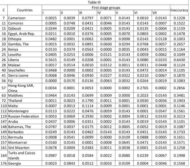
5.2.

O

Table III shows the twenty-seven outliers that were detected (see section 2.3.3). Second stage group

1101111 Rice

1101112 Other cereals, flour and other products 1101181 Sugar

1101113 Bread

1101114 Other bakery products 1101115 Pasta products 1101121 Beef and veal 1101122 Pork

1101123 Lamb, mutton and goat 1101124 Poultry

1101125 Other meats and meat preparations 1101131 Fresh, chilled or frozen fish and seafood 1101132 Preserved or processed fish and seafood 1101141 Fresh milk

1101142 Preserved milk and other milk products 1101143 Cheese

1101144 Eggs and egg-based products 1101151 Butter and margarine

1101153 Other edible oils and fats 1101161 Fresh or chilled fruit

1101171 Fresh or chilled vegetables other than potatoes 1101172 Fresh or chilled potatoes

1101162 Frozen, preserved or processed fruit and fruit-based products

1101173 Frozen, preserved or processed vegetables and vegetable-based products

1101182 Jams, marmalades and honey

1101183 Confectionery, chocolate and ice cream 1101191 Food products nec

1101211 Coffee, tea and cocoa

1101221 Mineral waters, soft drinks, fruit and vegetable juices Table II

ICP food and nonalcoholic beverages basic headings

1 2 3 4 5 6 7