Effect of temperature in oxygen consumption and body mass condition during a starvation period in the Peppery furrow shell – Scrobicularia plana (da Costa)

d

Ef

consu

during

S

ffect o

umptio

a star

Scrobic

D

F

of tem

on and

rvatio

furro

cularia

issertaç

Engenh

FILIPE C

VILA

peratu

d body

on peri

ow sh

ia

plan

ção de

haria Zoo

CORRE

A REAL, 2

ure in

y mas

iod in

hell –

na

(da

Mestrad

otécnica

EIA LINO

2010

oxyg

ss con

the P

Costa

do

O

en

dition

Pepper

a)

n

ry

Júri de Apreciação

Acknowledgements

I would like to express my gratitude to Silvia Santos and Dr. Henk van der Veer, and all the other research colleagues who made my internship at NIOZ a very nice experience.

I am very grateful to my teacher Dr. Paulo Rema, who coordinated the thesis preparation, for the involvement, support, help and patience.

At last and the most important gratefulness, to my mother and to my father that always encourage me despite the difficulties and arguments.

Preface

This report is the result of an internship at the Dutch Royal Institute for Sea Research (NIOZ), Texel, the Netherlands. It was an integrate part of the PhD project titled “Physiological performance of the Peppery furrow shell Scrobicularia plana (da Costa 1778) along the European coast”. This project aims to fill the gap in the scientific knowledge about how the species will be affected by environmental changes such as the ones associated with climate change (increased temperature stress).

The first part of the report consists in the state of the art of estuarine and coastal zone ecosystems. The second is a bibliographic review about Scrobicularia plana (da Costa, 1778) taxonomy, morphology, habitat, life cycle and ecological significance. In the third part, the experimental study about the effect of temperature in oxygen consumption and body mass condition is presented and the results described. The fourth and last part presents the discussion of the results and conclusions.

Table of Contents

Page number

Summary

Sumário

I.

Introduction

1. State of the Art……… 3

2. Taxonomy………... 5

3. Morphology………. 5

4. Habitat………. 6

5. Life Cycle……… 9

6. Ecological Significance………... 11

II.

Experimental study

1. Introduction………. 12

2. Material and Methods……….………….…………. 13

2.1. Sampling………. 13

2.2. Acclimation period……….……… 13

2.3. Feeding solution……….. 14

2.4. Water baths……….. 14

2.5. Sterilized sediment……….. 14

2.6. NO2; NO3; NH3/NH4+ water control tests………... 14

2.7. The setup………. 15

2.8. Water collection……….. 15

2.9. Glass bottles……… 15

2.10. Chemicals preparation………. 16

2.11. Absorbance measurements.………. 16

2.12. Ash-free dry matter determination……….. 17

2.13 Statistical analysis 17 3. Results………. 18

3.1 Relation between oxygen concentration in water (µmol/L) and oxygen consumption (µmol/h) over days of starvation, at the temperatures of

8ºC, 12 ºC, 15 ºC, 20 ºC and 24 ºC……… 19

3.2. Relation between body mass (mgAFDM.cm-3) over starvation period (days) at different temperatures (ºC)……….

24

4. Discussion / Conclusion………. 25

III.

References

Tables

Effect of temperature (ºC) in body mass condition (mgAFDM.cm-3) – ANOVA 24

Charts

Chart 1 - Means of overall oxygen consumption (µmol/h) at different temperatures (°C)  ₁₈ Chart 1 - Means of oxygen concentration (µmol/L) in water at 8ºC, during starvation

period. 

19

Chart 3 - Average oxygen consumption (µmol/h) at 8ºC, during starvation period.  ₁₉ Chart 4 - Means of oxygen concentration (µmol/L) in water at 12ºC, during starvation

period. 

20

Chart 5 - Average oxygen consumption (µmol/h) at 12ºC, during starvation period.  ₂₀ Chart 6 - Means of oxygen concentration (µmol/L) in water at 15ºC, during starvation

period 

21

Chart 7 - Average oxygen consumption (µmol/h) at 15ºC, during starvation period. 21

Chart 8 - Means of oxygen concentration (µmol/L) in water at 20ºC, during starvation period 

22

Chart 9 - Average oxygen consumption (µmol/h) at 20ºC, during starvation period 22

Chart 10 - Means of oxygen concentration in water (µmol/L) at 24ºC, during starvation period.

23

Chart 11 - Average oxygen consumption (µmol/h) at 24ºC, during starvation period. ₂₃ Chart 12 - Body mass (mgAFDM.cm-3) variation with temperature (ºC) 24

S

ummary

Oxygen consumption and body mass condition were studied in 30 animals during a starvation period. Animals were divided in 5 groups, 6 individuals each and a blank, and submitted to temperatures of 8ºC, 12ºC, 15ºC, 20ºC and 24ºC. Water samples were taken and oxygen concentration in water was measured, after an 8 hours period of enclosure, following the Winkler method (1888). To test differences between treatments, data were subjected to a one-way analysis of variance (ANOVA).

Results show oxygen consumption incresing with the increase of temperature with the highest consumption mean registered at 24ºC (5,559 µmol/h) and the lowest at 8ºC (0,780 µmol/h). At 8ºC, 12ºC, 15ºC and 20ºC, differences between oxygen consumption do not seem to be distinguishable for the short period of starvation. At 24ºC a peak of oxygen consumption was noticed at day 8 of starvation followed by a gradual decrease over time. Considering body mass condition (mgAFDM.cm-3), results show that temperature affects S. plana performance. It is shown that at higher temperatures, animals body mass have a higher decline over starvation than at lower temperatures, with no significant (p<0,05) changes in body mass condition detected for temperatures of 8ºC, 12ºC, 15ºC and 20ºC. Only at 24ºC, the changes were significant (p>0,05), with the body mass condition being influenced by temperature at the starvation period.

Sumário

O consumo de oxigénio e a condição corporal foram estudados para um grupo de 30 animais submetidos a um período de jejum. Os animais foram divididos em 5 grupos, 6 indivíduos cada grupo, a temperaturas de 8ºC, 12ºC, 15ºC, 20ºC e 24ºC. Foram colhidas amostras de água e medidas as respectivas concentrações de oxigénio, após 8 horas de consumo, seguindo o procedimento sugerido por Winkler (1888), “Winkler method”. Os dados obtidos foram tratados e submetidos a ANOVA.

Os resultados mostram que o consumo de oxigénio aumenta com o aumento da temperatura. A média de consumo mais elevada foi detectada a 24ºC (5,559 µmol/h) e a mais baixa a 8ºC (0,780 µmol/h). Às temperaturas de 8ºC, 12ºC, 15ºC e 20ºC, as diferenças registadas entre consumos de oxigénio não são significativas. À temperatura de 24ºC, registou-se um pico de consumo de oxigénio ao oitavo dia sem alimento seguido de um abaixamento gradual ao longo do tempo. Tendo em conta a condição da massa corporal (mgAFDM.cm-3), os resultados mostram que a S. plana é afectada pela temperatura. A temperaturas mais altas, a condição de massa corporal dos animais apresenta um decréscimo mais acentuado do que a temperaturas mais baixas, durante o período de jejum, não se registando alterações significativas (p>0,05) as temperaturas de 8ºC, 12ºC, 15ºC e 20ºC. Apenas a 24ºC foram detectadas diferenças significativas (p<0,05), e a condição de massa corporal foi influenciada pela temperatura durante o período de jejum.

I – Introduction

1. State of the Art

Among the most ecologically and socio-economically important environments on Earth are coastal zone ecosystems. They constitute valuable resources for agriculture, fisheries, navigation routes, industry settlement and recreational purposes (Kennish, 2002; Paerl, 2006). Many of the most important industrial, commercial and highly densely populated urban centres have been established, for many centuries, near estuaries along coastlines all over the world. Coastal zone ecosystems have high productivity, are crucial in the life histories of many fish, invertebrates, birds, etc. (McLusky, 1989) but are extremely fragile due to increasing stress from urbanization in coastal areas, intensive agriculture, mass tourism and pollution (Martinez et al., 2007). Human activities often lead to severe ecological stress and endangering the ecosystems and the disappearance of species from coastal marine environments is increasing. Nowadays, eutrophication is one of the major threats that these habitats have to face (Paerl, 2006). As a result of high nutrient input derived from urban, agricultural and industrial effluents, phytoplankton and macroalgal growth is stimulated, due to the particular characteristics of these systems (Kennish, 2002; Mclusky and Elliott, 2004; Lillebø et al., 2005, 2007; Dolbeth et al., 2007). In fact, one of the most frequent symptoms/consequences of eutrophication is the occurrence of macroalgal blooms (Raven and Taylor, 2003; Lillebø et al., 2005; Cardoso et al., 2008; Dolbeth et al., 2007). These events usually result in oxygen depletion, both in the water column and in the sediment, and consequent hypoxia and anoxia conditions, related to algal death and decay, having severe impacts on the system (Bolam et al., 2000; Pardal et al., 2000; Raven and Taylor, 2003; Verdelhos et al., 2005; Cardoso et al., 2008).

Declines in seagrass beds are often associated with increased eutrophication, resulting from the complex interaction of mechanisms such as changes in water and sediment quality (Bolam et al., 2000), smothering by algal mats (den Hartog and Phillips, 2000) and light and nutrients competition (Niehuis, 1996). Global awareness upon these problems has increased during the last decades, focussing on the assessment and protection of the ecological status of these ecosystems. Conservation and restoration have then become a priority, in order to return a system from an altered or

disturbed condition to a previously existing stable state condition (de Jong and de Jong, 2002; Kendrick et al., 2002; Webster and Harris, 2004). These ecosystems face another worldwide major problem: the increased climate variability associated with global warming. Climate is expected to affect the performance of individuals, populations and communities, with diverse geographical distributions (Short and Neckles, 1999; Simas

et al., 2001; Adams, 2005; Harley et al., 2006). It is then extremely important to

understand the wide complexity of the climate change problem, its causes, the mechanisms involved and worldwide impacts. Studies on population and community level processes are thus required for a holistic and integrative view of the ecosystems response to global climate change.

In recent years there has been an upsurge of interest in climate change impacts in marine systems, and some studies have been conducted focusing on temperature (Harley

et al., 2006), and on the impact of large scale weather events, such as flooding, droughts

and heat waves, on the functioning of macrobenthic communities (Norkko et al., 2002; Salen-Picard and Arlhac, 2002; Salen-Picard et al., 2003). According to Norkko et al. (2002), catastrophic clay deposition associated with severe flooding, can have markedly deleterious effects on estuarine macrobenthic communities. Other studies have shown an increase in the density of opportunistic species after flood events (Salen-Picard and Arlhac, 2002; Salen-Picard et al., 2003).

Benthic fauna living in close contact with sediments are particularly exposed to chemical stress. In direct contact with sediments, through ingestion of sediment particles and physical contact, benthic fauna species are a suitable indicator of sediment-associated contaminants (Bryan et al., 1985; Byrne and O’Halloran, 2001). Bivalves are among the most productive groups of infaunal organisms (Mistri et al., 2000; Cusson and Bourget, 2005; Dolbeth et al., 2007). They play a key role on the ecosystem, as an essential link between the primary producers and epibenthic consumers, filtering organic matter, purifying the water column and influencing the food availability and energy flow on the entire community (de Montaudouin et al., 1999). Moreover, they form an important part of the diet of wading birds, crabs and benthic fish (Hughes, 1969) and if contaminants are available, they can be transferred through the food chain. Therefore, studies about biological cycle and how the climate changes will affect the maintenance, growth and development of benthic species need to be formulated in order to achieve the desire knowledge about the performance of these species in the future.

This is the case of Scrobicularia plana which has disappeared from many locations during the past two decades (Thiel et al., 1998). Scrobicularia plana (da Costa, 1778) is a bivalve specie very important in shallow water benthic communities (Keegan, 1986), with a wide distributional range and commercially exploited in several countries (Hughes, 1970). It ranges from the Norwegian Sea to the Iberian Peninsula, into the Mediterranean, along the Atlantic coast of Morocco, the Canary Isles and south to Senegal (Tebble, 1976). S. plana is also characterized by a high tolerance to physical and chemical changes in the sediment and rapid demographic adaptability to variations in the environment (Hughes, 1970; Nott, 1980).

2. Taxonomy

Scrobicularia plana, commonly named as peppery furrow shell, is inserted in the

Phylum Molusca, Class Bivalvia. Bivalves have a shell consisting of two asymmetrically rounded halves called valves, typically bilaterally symmetrical, with the hinge lying in the sagittal plane. It belongs to the Order Veneroida, as some other well-known bivalves such as saltwater clams and cockles, which are characterized as thick-valved, equally thick-valved, and adductor muscles of the same size (Scarlato, 1979).

Scrobicularia plana belongs to the Superfamily Tellinoidea, but there is not a general

consensus about the taxonomy of this specie. Some authors integrate S. plana in the Family Semelidae (ITIS, NHM) and others refer to it as a sole genus belonging to the Family Scrobiculariidae (MarLIN, WoRMS).

3. Morphology

The peppery furrow shell is a bivalve mollusc with a thin, flattened and rounded shell that grows up to 6.5 cm in length. The outer surface of the shell may be white, grey or yellowish, and has fine concentric lines; the inside is always white (Pizzolla, 2002). Internal features for identification are the hinge of the valves (the right valve has two teeth and the left valve one tooth), each one supported by a direct chondophore (Hayward and Ryland, 1990), and a broad and almost circular pallial sinus, a U-shaped dip in the pallial line near the posteroventral margin of the shell which represents the attachment scar of the siphon retractor muscles. It allows the siphons to be withdrawn into the shell before closing the shell (Pizzolla, 2002). The adductor scars and pallial

line are not clearly visible in fresh material. Pallial line is linked with the lower edge of a wide pallial sinus, although cruciform muscle scars may be apparent (Hayward and Ryland, 1990)

According to Pizzolla (2002), S. plana almost perfect flatness is a distinguishable morphological characteristic to other bivalve species.

4. Habitat

The Peppery furrow shell, Scrobicularia plana, is a long-lived deposit-feeding bivalve species with a broad geographic distribution, being present in several European estuaries (Hughes, 1970; Guelorget and Mazoyer-Mayére, 1983; Essink et al., 1991; Sola, 1997; Guerreiro, 1998). It has a wide distributional range, being present from the Norwegian Sea to Senegal, in the Atlantic Coast, and also in the Mediterranean Sea (Tebble, 1976). It inhabits the intertidal coastal waters in great abundance and is often the dominant species of shallow water benthic communities (Tebble, 1976; Keegan 1986). S. plana shows highest densities in the intertidal muddy and muddy sand zones (Borja, 1988), being an abundant and important species in the estuarine trophic chain (Ruiz et al., 1995). It can also be an important link in the food chains of estuaries and coastal lagoons (Hughes, 1970; Bachelet, 1982; Guerlorget and Mazoyer-Mayere, 1983). Scrobicularia plana is an important prey species for several fish and marine birds (Hughes, 1970; Zwarts and Wanink, 1989). A significant percentage of mortality among juveniles is due to predation by flatfish, shrimp, crabs (Zwarts and Wanink, 1989) and birds (Hughes, 1970). This bivalve burrows into the sediment to depths of around 20 cm. When covered by the tide, it feeds by extending its inhalant siphon to the surface; a current of water passes down the siphon and into the body of the bivalve, where particles are removed. The water is then expelled via the exhalant siphon. It feeds on surface matter of the sediment, and leaves star-shaped marks where it has been feeding (Fish and Fish, 1996). Although they primarily suck up surface deposits, S.

plana obtain some of the food by filtering suspended matter from the water column

(Hughes, 1970; Hughes, 1973). Many estuarine bivalves loose the siphon tips because of "cropping" predators. Crabs and fishes often feed on the inhalant siphon when it is extended, but the damaged tissue is replaced quickly, in around 5 days (Fish and Fish, 1996). Their most effective means of protection is to increase burial depth and, as a

result, quick growth to increase siphon mass seems to take priority over reproduction (Zwarts and Wanink, 1989).

In many coastal waters, benthic macrophytes form large dense stands from late spring to early autumn. Often only a small proportion of this biomass is directly consumed by herbivores; the remaining part enters the detritical pool and becomes available to deposit-feeders. Living micro-organisms are commonly much better absorbed than detritus, suggesting that they constitute the main food source of deposit-feeding bivalves (Matthews et al., 1989). S. plana plays an important role in the coupling between the benthic and pelagic systems by removing large amounts of particulate material from the water column (Alpine and Cloern, 1992), partly sequestrating the nitrogen and phosphorus (Nalepa et al., 1991) and releasing inorganic nutrients into the water column from direct excretion and production of pseudofaeces (Prins and Smaal, 1994). The sediment enrichment with biodeposits provides a nutrient source for other biotic components such as macrophytes and epibenthic deposit-feeders (Casagranda and Boudouresque, 2005).

Environmental factors affect the marine invertebrates’ distribution (Peterson, 1991; Warnick et al. 1991). Food availability (Beukema et al. 1977; Peterson and Black, 1987) influenced by shore elevations (Peterson and Black, 1987; Beukema and Flach, 1995), as well as physiological stress (Peterson, 1991), water temperature (Beukema et al., 1985) and sediment grain size (Beukema and Flach, 1995) have been reported as the main factors of the variations in distribution and biomass of S. plana in intertidal areas (Thrust et al., 1989; Turner et al., 1995). Also predation (Holland et al., 1980) and intra- and interspecific competition (Beukema and Flach, 1995) can have an effect on these populations. Furthermore, Hughes (1970) suggests that S. plana has no territorial effect due to the frequently overlap and close juxtaposition while deposit feeding with no effect on each other’s activities.

S. plana is characterized by a high tolerance to physical and chemical changes in

the sediment and rapid demographic adaptability to variations in the environment (Hughes, 1970; Nott, 1980). Temperature is considered to be the most significant physical factor and has an important role in distribution patterns, physiological rates and reproductive cycles, being the air temperature as influent as the water temperature (Hayward and Ryland, 1995). In the winter, when the growth is stopped or very slow (Jensen, 1992; Guillou and Tartu, 1994), it buries twice deeper in the sediment than in

summer (Zwarts and Wanink, 1989). Scrobicularia plana reaches higher abundances in more southern areas, like Aiguillon Bay in France (Bocher et al., 2007).

On the other hand, S. plana has high tolerance to salinity variances that can range from 1-2‰ (Green, 1957) to 34.5‰ (Freeman and Rigler, 1957), although it closes the valves at salinity values of approximately 20‰ (Akberali and Davenport, 1981). This demonstrates the greater tolerance to salinities variations comparing with other estuarine species like Macoma balthica, Mytilus edulis and Cerastoderma edule (Bryan and Hummerstone, 1977). The bivalve molluscs Scrobicularia plana (da Costa) and Mytilus edulis L. both respond to falling external salinities by detecting changes in the concentration of a group of ions (rather than to osmotic pressure changes or changes in the concentration of a single ion). Scrobicularia is sensitive to Na+, Mg2+, Ca2+ (and possibly Cl−). The salinity sensing structures are deeply situated in S. plana, in contrast to the peripheral location in Mytilus (Akberali and Davenport, 1981). Hughes (1970) suggests that S. plana can tolerate such conditions by clamping the shell valves together, isolating the tissues and body fluids from the water column, until better conditions become available. These characteristics show the adaptive ability of the animal to survive in varying salinity, even considering their low mobility (Akberali, 1978).

Notwithstanding, S. plana have a wide distribution over the North Atlantic and Mediterranean coastal zones, with higher densities at southern areas observed. Bocher et

al. (2007) reported a 3,055 individuals.m-2 in Gironde estuary (France), Sola (1997)

found 5.892 indivuduals.m-2 in Bidasoa estuary (North Spain), whilst Casagranda and Boudouresque (2005) calculated mean densities of 299 to 400 individuals.m-2 in Ichkeul wetlands (Tunisia), during a ten month period study. Some authors defend local factors for these results, such as: sediment stability (Sola, 1994), very significant for the development of deposit-feeding species (Wolff, 1973; Bachelet, 1980); sediment richness on organic matter, benefiting the bacterial development (Dale, 1974), basis of deposit-feeding diet (Lopez and Levington, 1987); and the small proportion of predators and bivalve competitors (Sola, 1997; Casagranda and Boudouresque, 2005).

Langston et al. (1987) and Essink et al. (1991) reported a decreasing tendency over Scrobicularia plana populations. An increment of severe winters, sediment instability and pollution should be seen as major threats to this phenomenon (Essink et

al., 1991; Thiel et al., 1998). Ruiz et al., (1994) discover that tributyltin (TBT), the

European estuaries, should be responsible for the abnormal development of embryonic and larvae stages of S. plana, delaying their reproductive cycle. Therefore, the chances of a successful reproductive cycle decrease, while predation, dispersal and diseases increase.

5. Life Cycle

S. plana is often characterized as a gonochoristic specie (Hughes, 1971;

Guerreiro, 1991; Ruiz, 1991; Sola, 1994), however Paes-da-França (1956) and Raleigh and Keegan (2006) reported a few cases of hermaphroditism. According to Lammens (1967), in gonochoristic bivalve species, hermaphroditism can occur but in a very low percentage.

Regarding the reproductive cycle, S. plana only reaches sexual maturity in the second summer of life (Hughes, 1971), corresponding to an approximately shell length of 20cm (Paes-da-França, 1956; Bachelet, 1981; Sola, 1997; Guerreiro, 1998; Rodríguez-Rua et al., 2003; Raleigh and Keegan, 2006). The gonadal development occurs after a year of sexual reserves storage, mainly during summer and autumn and maintained during winter. The spawning takes place in the following spring and summer (Paes-da-França, 1956; Hughes, 1971). However, Scrobicularia’s reproductive cycle varies with latitude, in which the southern populations present more than one annual period (Paes-da-França, 1956; Hughes, 1971; Bachelet, 1981; Guerreiro, 1998). Studies reveal three different patterns of reproduction along the European Coast: one period per year, mostly in northern areas (Lebour, 1938; Stopford, 1951; Hughes, 1971; Rasmussen, 1973; Warwick and Price, 1975; Worrall et al., 1983), two periods per year, in the Gironde estuary, Bay of Arcachon (Bachelet, 1981) and Tagus (Paes-Da-Franca, 1956), and one prolonged period per year, in the Mira and Tagus estuaries (Silva, 1991). Worall et al. (1983) suggests that differences in the breeding cycle timing and length are due to food availability. Thus, the lowest the food is available, the fastest the gametes develop and the earliest the spawning occur. Also temperature is reported as an influencing factor, whereat the increasing of temperature after winter can be a factor of the gametogenesis’ inception (Sastry, 1970).

S. plana spawns to the water column, in a continuous process and not all at once

(Raleigh and Keegan, 2006), although the number of eggs produced and spawned is not studied yet or is not available in literature. The larvae have a planktotrophic

development with a long pelagic stage (Hughes, 1970). The larval development is divided in two stages: from hatching to pediveliger larvae, wherein veligers dwells in pelagic environment, and from settlement to complete metamorphosis, when individuals appear buried in the sediment top millimeters, although, they often return to the water column. These are the stages where colonization of other areas is more presumable (Ruiz et al., 1995). They undergo metamorphosis into adults and settle after this planktonic stage, which lasts for 2 or 3 weeks (Fish and Fish, 1996). At this time, they develop the siphons and start to grow through deposit-feeding (Ruiz et al., 1994). Due to the short siphon size, they settle within the top 5cm of the surface, what makes them vulnerable for predators and extreme cold or heat, turning mortality rates higher (Hughes, 1970; Ruiz et al., 1994; Casagranda and Boudouresque, 2005).

Growth patterns are not entirely clear and can vary with age, location and season. In South Wales, Green (1957) reported a growth of 5mm.year-1 in the first three years, an increase to 7mm.year-1 in the next two years, and a progressive decline till 2mm.year-1 _{at the tenth winter. On the other hand, in Spain, Sola (1997) observed a fast}

growth in the first 16 month, with shells reaching approximately 21mm length and, within a year, growing up to 30mm. Verdelhos et al. (2005) estimated a growth rate of 10mm.year-1 in Mondego estuary (Portugal). Energy balance between energy intake, relative to food availability and consumption, and energy demands, depending mostly on temperature, is the cause of seasonal variations (Zwarts, 1991).

Despite having vast longevity, populations in southern areas have a shorter lifespan, wherein Verdelhos et al. (2005) and Coelho et al. (2006) recorded an approximately five years’ life span. Also age determination is more difficult in these areas because winters are not as rigorous as in northern countries, with an insufficient decrease in metabolic rates, responsible for the yearly rings formation (Hughes, 1970; Sola, 1997).

6. Ecological Significance

Deposit-feeders bivalves base their diet on bacterial population, whose development depend on the sediment’s organic matter content (Lopez, 1987). But S.

plana can also be a filter-feeder who, at high tide, feed on suspended matter such as

phytoplankton (Hughes, 1969). According to Riera et al. (1999), Scrobicularia have a diet based on 2/3 of deposit-feeding and 1/3 of suspension-feeding. When feeding, S.

plana extend the siphon up to 5cm in the sediment, taking the risk of being eaten by

predators, although whenever there is a vibration on the mud, they quickly withdraw the siphon (Hughes, 1969). However, sometimes this reaction is not quick enough, and some wading birds, mostly the oystercatcher Haematopus ostralegus L. can crop the siphon (Hughes, 1969; Zwarts, 1991). Cod and fresh-water eels (Hughes, 1970), as well as black-tailed godwits, dunlins, black-header and black-backed gulls (Moreira, 1997) are other predators examples.

Bivalves are able to regenerate the siphon (Trevallion, 1971; de Vlas, 1979; Hodgson, 1982), but it brings plenty of negative consequences. Reproduction and gonadal development (Trevallion et al, 1970; Trevallion, 1971), body condition (Trevallion et al, 1970; Trevallion, 1971; Hodgson, 1982) and somatic growth (Peterson and Quammen, 1982) are the most affected physiological activities. The amputation of the siphon obliges bivalves to live closer to the surface, what put them in a higher risk of being eaten by birds (Zwarts and Warnick, 1989).

II - Experimental study

1. Introduction

The objective of the experimental study was to measure Scrobicularia plana (da Costa, 1778) oxygen consumption rates, at different fixed temperatures, during a starvation period. Animals were collected to the laboratory and data was registered and analysed. The methodology choice was based in resources availability, accuracy and cost-effectiveness, whence the Winkler method (Winkler 1888) seemed to be the most appropriated to measure dissolved oxygen in water.

In the Winkler method, manganese chloride is added to a known amount of seawater, followed by the addition of an alkaline sodium hydroxide-potassium iodide solution. The resulting manganous hydroxide precipitate reacts with the dissolved oxygen in the water and forms a hydrated tetravalent oxide of manganese. Upon acidification, the manganese hydroxides dissolve, and the tetravalent manganese acts as an oxidizing agent and liberates iodine from the iodide ions. The iodine is equivalent to the dissolved oxygen in seawater and present as free iodine (I2) and tri-iodide (I3–)

(Burger and Liebhafsky, 1973).

In the Winkler method, the iodine is determined titrimetrically with standard thiosulfate; however, despite improved automation of the end-point detection (Bryan et

al., 1976; Williams and Jenkinson, 1982; Furuya and Harada, 1995), it commonly takes

4 to 6 min to titrate a sample. A faster spectrophotometric approach to determine O2

was introduced by Broenkow and Cline (1969) and is based on measuring the absorbance of the colour I2 and I3–. The concentration of oxygen is then calculated by

comparing the absorbance in a sample against standards of known oxygen content made from potassium iodate (KIO3) solutions.

2. Material and Methods

2.1 Sampling

Animals were collected in Westerschelde, Terneuzen, the Netherlands (51° 24′ 0″ N, 3° 43′ 0″ E). Individuals were collected by digging out (hand digging) the top 20cm of the sediment. Only animals with shell length size between 25.59 and 27.36mm were taken. The size class range was calculated from a starting length of 26.50mm, which was then converted to volume using the equation:

V = (δ*L)3

where V is the volume (ml), δ is the shape factor for the species in Terneuzen and L is the length (mm) (van der Veer et al., 2006); the final range was determined by considering +/- 10%V.

Thirty animals were collected and transported, in a cooler (± 5ºC), to the laboratory. Animals were randomly divided in 5 groups of 6 animals. Each group was placed in different aquariums inside five water baths, and fed ad libitum.

2.2 Acclimation period

The experiment took place in two climate rooms at pre-set air and water temperatures of 8° and 15°C. In the room at 8°C, two water baths were set (8ºC and 12ºC), while the remaining three were in the room at 15°C (15ºC, 20ºC and 24ºC). To achieve the desired temperatures, water baths were heated with commercial aquariums heating system (Hydor Theo® 100W): from 8°C to 12°C and from 15°C to 20°C and 24°C. Temperatures were controlled with commercial aquarium thermometers (MORE®), one in each water bath. The water was continuously aerated with oxygen pumps available in the climate rooms. The feeding solution flow was adjusted to 1 litre per day per aquarium in order to fulfil the nutritional requirements. The animals were kept like it was described, about 10 days before the starvation period and the water collection start.

2.3 Feeding solution

The feeding solution was released to each aquarium by a pump (Gilson Miniplus 2), from a 5 litres Erlenmeyer. The feed used was a mix of four marine microalgae labelled as Shellfish Diet 1800® (Instant Algae®) that can be used as a complete live algae replacement (1 quart of Shellfish Diet replace the equivalent to 1800 litres of dense algae culture). The cell count is roughly 2 billion cells per ml. The feeding solution was: 2.5ml of the algae mix to 5 litres of filtered seawater. Each aquarium was fed 1 litre of this solution per day.

2.4 Water baths

The water baths consisted in a big container (≈40 m3) filled with filtered sea water. The temperature was previously increased, until the temperatures of 8°, 12°, 15°, 20° and 24°C were reached for each bath. The water had a continuous flow, allowing overflowing. An aquarium of about 3 litres was placed inside each container during the acclimation period. In the aquarium, a 5cm layer of sediment was placed to allow the animals to bury themselves.

2.5 Sterilized sediment

Since the animals needed to be kept under starvation conditions after the acclimation period, the sediment could not have any organic matter. The sediment was collected at the beach in Den Hoorn (Texel) and, in order to remove any organic matter, it was burned at 580°C in a vacuum oven for 4 hours and kept under sterilized conditions (to prevent contamination) until the experimental setup.

2.6 NO2; NO3; NH3/NH4+ water control tests

During the experiment, tests were performed to assess water quality. The tests used were the commercial control tests (SERA®) for NO2, NO3, and NH3/NH4+. These

tests were performed once a week and all the results were in the ideal range for the specie.

2.7 The setup

For the measurements, length, width and height of each individual were registered. Then, each animal was removed from the aquariums to an individual numbered flask with 800ml volume. The flasks had a 5cm layer of sterilized sediment (± 546 g) and the animal was buried into the sediment. The flasks were then placed inside the correspondent water bath, 6 per temperature plus one control flask (blank). The control flask consists on the same quantity of sterilized sediment but without animal inside. At this time, the feeding solution was taken out and the animals start the starvation period.

2.8 Water collection

Collections were performed during a 4 weeks period, with an average of two per week. For each sample, the flasks were closed with a cap for a period of 8 hours. The cap was drilled in the middle and sealed with a plastic cork. The drilling was necessary to remove the water from the flasks through an 8mm PVC tube (TYGON®), without air contamination. The water was collected to glass bottles with a volume of about 120 ml, allowing the overflowing before capping. After the 8 hours period, water samples were collected from inside the flasks. Two replicates of each flask were collected.

2.9 Glass bottles

Custom-made oxygen bottles made from borosilicate glass with a nominal volume in the range of 116 to 122 cm3 were calibrated to the mm3 level according to the recommendations of the World Ocean Circulation Experiment (WOCE) (Culberson, 1991). Each borosilicate glass bottle and the corresponding ground-glass stopper were engraved with a unique number for later identification of the exact volume. About one hundred bottles were used to prepare the calibration standards.

2.10 Chemicals preparation

Common Winkler reagents were used to determine oxygen concentrations: manganese chloride (MnCl2·4H2O; 600 g dm–3; 3 mol L–1) (reagent A), alkaline iodide

reagent (NaOH; 250 g dm–3; 6 mol L–1 + KI; 350 g dm–3; 2 mol L–1) (reagent B), and sulphuric acid (H2SO4; 10 mol L–1) (reagent C). After preparation, the reagent-grade

chemicals were filtered through Whatman GF/F filters and subsequently stored in polycarbonate bottles at ~20°C in the dark. The standard stock solution was prepared with potassium iodate (KIO3) (Malinckrodt Baker; primary standard). KIO3 was dried at

180°C for 6 hours, and 2.5 g KIO3 was dissolved in 250 cm3 ultrapure Milli-Q water. The prepared stock solution was divided into small 50-mL polycarbonate bottles and stored in a chamber with 100% humidity to prevent evaporation of water and therefore an increase in the concentration of the stock solution over long storage periods.

2.11 Absorbance measurements

Water was siphoned into the glass bottles through a laboratory grade PVC tubing (TYGON®), overflowing each bottle by at least 2 times its volume. The oxygen content in a bottle was fixed with 1 cm3 reagent A, followed by 2 cm3 reagent B, both added near the bottom of the bottle with high-precision dispensers (Fortuna Optifix basic; precision ± 0.1%). The precise addition of chemicals (A) and (B) is important because they dilute the sample. After adding the reagents, the bottles were stoppered and hand-shaken vigorously to mix the chemicals. The addition of reagents and stoppering of the bottles were done as quickly as possible to prevent contamination of undersaturated samples by atmospheric oxygen. For incubation and storage, the bottles were immersed in water baths (kept at in situ temperature) to avoid drying of the stopper seal. About 20 minutes after, the fixed bottles were shaken again to ensure complete reaction of the chemicals. Before starting the absorbance measurements, 1 cm3 reagent (C) was added to the fixed samples. Subsequently, a small magnetic stirring bar was introduced carefully, and the bottle openings were covered with parafilm to avoid loss of volatile compounds. The samples were gently stirred for a few seconds with an external magnetic stirrer (Metrohm) until the precipitate in the bottles was dissolved. Then, the absorbance was measured in a spectrophotometer (LKB Biochrom - England) at a wavelength of 456nm (Labasque et al., 2004). Data were registered and quantified.

2.12 Ash-free dry matter determination

Ash-free dry mass (AFDM) was determined to the nearest 0.01 mg, as the difference in dry and ash mass by first drying each part for 48 hours at 60°C followed by incineration for 2 hours at 580°C.

2.13 Statistical analysis

Data are presented as means ± standard deviation. To test differences between treatments, data were subjected to a one-way analysis of variance (ANOVA) and when appropriate, means were compared by the Newman-Keuls multiple range test. Statistical significance was tested at a 0.05 probability level. All statistical tests were performed using the XLSTAT statistical package.

3. Results

Oxygen concentrations (µmol/L) were calculated via software (Microsoft Access®) with the following simplified equation:

[O2] (µmol/L) = (Esamp – Eturb) / k * Vc / (Vc – Vr) – 0.65 – “chemical” blank; where:

Esamp = absorbance of the sample

Eturb = absorbance of the glass bottle

Vc = glass bottle volume

Vr = total volume of reagents A + B

The absorbance of the glass bottle (Eturb), the “chemical” blank and the k value

were already calculated and included in the software database.

On the other hand, oxygen consumption (µmol/h) was calculated for each group and means of each group (n=6) at different temperatures (ºC) were compiled in chart 1.

Chart 1- Means of overall oxygen consumption (µmol/h) at different temperatures (°C)

The highest mean of oxygen consumption (µmol/h) observed was 5,559 at 24°C, and the lowest was 0,780 at 8°C. The relation between data seems to be linear, with the oxygen consumption incresing with the increase of temperature.

For the statistical analysis, means of oxygen concentration in water were calculated for each group (animals and blanks), at different temperatures and increasing days of starvation.

3.1 Relation between oxygen concentration in water (µmol/L) and oxygen consumption (µmol/h) over days of starvation, at the temperatures of 8ºC, 12 ºC, 15 ºC, 20 ºC and 24 ºC

Chart 2- Means of oxygen concentration (µmol/L) in water at 8ºC, during starvation period.

Chart 3- Average oxygen consumption (µmol/h) at 8ºC, during starvation period.

Animals at 8ºC presented oxygen concentration (µmol/L) values between 275,140 and 297,342 for a period of 25 days of starvation. The highest value was at day 15 and the lowest at day 12. Considering oxygen consumption (µmol/h), the values range is from 0,805 at day 12, to 0,075 at day 6.

Chart 4- Means of oxygen concentration (µmol/L) in water at 12ºC, during starvation period.

Chart 5- Average oxygen consumption (µmol/h) at 12ºC, during starvation period.

In this group, oxygen concentrations (µmol/L) range from 221,742 (day 12) and 266,534 (day 1) showing a superior range between values comparing to the previous group. Also oxygen consumption (µmol/h) had a higher variation, with values between 0,248 and 1,229, although the pattern is still not very clear.

Chart 6- Means of oxygen concentration(µmol/L) in water at 15ºC, during starvation period.

Chart 7- Average oxygen consumption (µmol/h) at 15ºC, during starvation period.

This group of animals shows values of oxygen concentration between 259,363µmol/L at day 11, and 232,638 µmol/L at day 1. The oxygen consumption (µmol/h) pattern is similar to the one presented by the group of animals at 12ºC, with values varying from 1,215 at day 1, to 0.598 at day 11.

Chart 8- Means of oxygen concentration (µmol/L)in water at 20ºC, during starvation period.

Chart 9- Average oxygen consumption (µmol/h) at 20ºC, during starvation period

At 20ºC, the oxygen concentrations (µmol/L) present a range with a higher value of 238,161 at day 1 and a lowest value of 177,620 at day 3. Considering the oxygen consumption (µmol/h), a superior variation is noticed, but the pattern is still not very clear. Values vary from 0,429 to 1,883 µmol/h.

Chart 10- Means of oxygen concentration in water (µmol/L) at 24ºC, during starvation period.

Chart 11- Average oxygen consumption (µmol/h) at 24ºC, during starvation period.

At 24ºC, oxygen concentration (µmol/L) in water present values between 191,819 at day 17, and 148,210 at day 8. The oxygen consumption (µmol/h) is higher than for other temperatures and it seems like there is a decrease over time, with a steep decline after day 8. Values range is from 2,973 at day 8, and 0,802 at day 21.

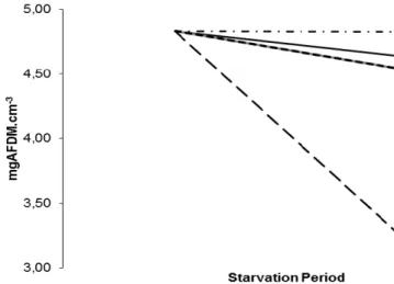
3.2. Relation between body mass (mgAFDM.cm-3) over starvation period (days) at different temperatures (ºC)

Table 1- Effect of temperature (ºC) in body mass condition (mgAFDM.cm-3) – ANOVA

Control 8ºC 12ºC 15ºC 20ºC 24ºC Body mass (mgAFDM.cm-3) 1 4,83a 4,64a 4,83a 4,54a 4,54a 3,26b

Standard deviation 0,57 1,20 0,48 0,60 0,37 0,25

1- mgAFDM.cm-3 = (AFDM*1000)/(lenght/10)3

Values are means ± standard deviation (n=6).

Within a row, means with different superscript letters differ significantly (P<0.05).

Considering the effect of temperature (ºC) in body mass condition (mgAFDM.cm-3), means range from 3,26 to 4,83 (Table 1). The group at 24ºC presents a significant decrease (p<0,05) of body mass condition comparing to all the other groups at inferior temperatures. This means that during a starvation period, at 24ºC, animals have higher weight losses than the ones at lower temperatures.

The groups at lower temperatures (8º, 12º, 15º and 20ºC) show no significant differences (p>0,05) comparing to the control group, which was kept under natural conditions.

  To compile this data, a chart with the information in Table 1 was delineated.

4. Discussion / Conclusion

The disappearance of species from coastal marine environments is a cause for concern. This is the case of Scrobicularia plana which has disappeared from many locations during the past two decades. Pollution has been discussed as the most important factor causing the local extinction of S. plana (Ruiz et al., 1994), but also predation (Holland et al., 1980) and global warming (Peterson and Black, 1987; Beukema et al., 1985; Beukema and Flach, 1995) have been considered. To better understand the mechanisms behind the disappearance of S. plana’s populations, knowledge about the physiological performance of the species in relation to environmental conditions is essential. However, at present, there is still a lack of basic information in that field.

One of the main environmental factors affecting physiological processes in marine species is temperature, with an important role in distribution patterns, physiological rates and reproductive cycles, being the air temperature as influent as the water temperature (Hayward and Ryland, 1995). In this work, the effect of water temperature (ºC) on Scrobicularia plana’s maintenance over a starvation period was studied in order to establish a relation on how temperature can affect oxygen consumption and body mass condition. That knowledge is essential to know how the species will react to environmental changes in temperature, namely the ones associated with climate change.

During the experiment all animals were consuming oxygen, denoted by the difference between blanks and the group mean water oxygen concentrations (µmol/L) at all temperatures. The group means of oxygen concentration in water ranges from 275,140 µmol/L to 297,342 µmol/L at the lowest temperature (8ºC), and from 148,210 µmol/L to 191,819 µmol/L at the highest temperature (24ºC); the blank ranges from 283,700 µmol/L to 302,090 µmol/L at 8ºC, and from 192,165 µmol/L to 215,990 µmol/L at 24ºC. A quick overlook after these results shows that the difference between blanks and group means is higher at 24ºC than at 8ºC. Since the filtration process removed all other organisms present in the seawater, and given that this was oxygen saturated, we can conclude that animals were consuming oxygen at different rates, with the lowest rate measured at the lowest temperature (8ºC). A likely explanation is that at low temperatures, animals reduce their metabolic rate, so they need less oxygen to fulfil

their requirements. Zwarts (1991) found a consistent relationship between temperature and metabolic rates with metabolic rates decreasing with a decrease in temperature. Our results seem to be in agreement with those findings with animals consuming less oxygen at 8ºC likely due to a lower metabolic rate. At temperatures of 12ºC, 15ºC, and 20ºC, an increased mean difference in oxygen concentration between group and blanks was detected, confirming the gradually increase of oxygen consumption (µmol/h) with temperature, which is expected to be related with an increase in metabolic rates.

When analysing each group over the time of the experiment, oxygen consumption (µmol/h) at these temperatures seems to be constant, and the differences between them do not seem to be distinguishable for the short period of starvation that animals were subjected. However, at 24ºC a peak of oxygen consumption (µmol/h) was noticed at day 8 of starvation followed by a gradual decrease over time. This suggests that at this temperature, the energy reserves of the animals allowed them to maintain a constant metabolic rate for 8 days after which a depletion of the reserves occurred and a decrease in the oxygen consumption rate (µmol/h) was observed. A similar pattern was expected for the groups at lower temperatures but later in time since maintenance costs are lower at lower temperatures. However that was not observed most likely due to the short duration of the experiment which did not allow the complete depletion of reserves at lower temperatures.

In conclusion, it seems that animals at temperatures of 8ºC have very low oxygen consumption (µmol/h) due to their low metabolic rate and, therefore, metabolic requirements. As the temperature increase, until 20ºC, the oxygen consumption increase gradually as well as metabolic requirements, but the differences do not seem to affect animals’ performance. At 24ºC, differences in oxygen concentration in water (µmol/L) between blank and group means are the highest. Also, at this temperature it took the animals around 8 days under starvation to deplete their reserves. Thus, animals were consuming more oxygen confirming that, at higher temperatures, the metabolic rate increase and the oxygen requirements are superior, in order to fulfil maintenance requirements. Moreover, under starvation conditions, the reserves are more rapidly consumed to the point when the animals do not have enough reserves to maintain a constant metabolic rate. Therefore, it seems that S. plana’s oxygen consumption (µmol/h) increase with the increase of temperature. Additionally, at a given temperature, animals keep their metabolic rates relatively constant until energy reserves are not enough anymore and rates begin to drop.

Considering body mass condition (mgAFDM.cm-3), results show that temperature (ºC) affects S. plana performance. It is shown that at higher temperatures, animals body mass have a higher decline over starvation than at lower temperatures. A decrease over time was observed for almost all temperatures. The decrease in body mass condition seems to be higher with increased temperature: at 8°C a minor decrease over time was observed; at 15°C and 20°C the values are very similar but presents a slight decrease when compared with the lowest temperature; the highest body mass losses were observed at the highest temperature (24°C). Only at 12ºC a very slightly increase in body mass was registered. As the initial values were taken from a control group, a possible explanation is that these animals presented an initial better condition than the control animals. However, all animals were collected at the exact same location and period, and corrected for shell size; therefore that explanation may not be very likely.

The decrease in body mass was expected, over a starvation period, due to lack of food the animal would use its reserves to obtain energy for maintenance (Hughes, 1970). Therefore, over time, reserves were used and consequently the body mass decrease. At higher temperatures, a more accentuated decrease was expected since the maintenance costs for the animal are also higher (Hughes, 1970).

In conclusion, no significant (p>0,05) changes in body mass condition (mgAFDM.cm-3) were detected for temperatures of 8ºC, 12ºC, 15ºC and 20ºC. Only at 24ºC, the difference was significant (p>0,05), and the decrease of body mass condition was influenced by temperature at the starvation period. This fact can be important, in terms of production and depuration, for molluscs’ farmers, as animals do not have significant weight losses in a wide temperature range (from 8ºC to 20ºC) and can be kept under starvation conditions, for at least 21 days, with the same performance.

Although some valuable information was obtained from this experiment, some setbacks happened with material availability and with setup arrangement that affected its outcome. Oxygen concentrations were calculated according to the Winkler method (Winkler, 1888) due to its accuracy and cost-effectiveness. However, the methodology is slow and involves plenty of time per each collection and measurement, and as a result only a small number of samples per week (about 2) were collected. Moreover, the short period of the experiments influenced the results, which did not allow making more realistic conclusions. Further studies should be made, with longer starvation periods,

higher temperatures and an easier and faster procedure to calculate oxygen consumption, in order to obtain better results.

III. References

Adams, S.M. (2005) “Assessing cause and effect of multiple stressors on marine systems”. Marine Pollution Bulletin vol.51 pp.649–657

Akberali, H.B. (1978) “Behaviour of Scrobicularia plana (Da Costa) in water of various salinities”. J. Exp. Mar. Biol. Ecol. vol.33(3) pp.237-249

Akberali, H.B., Davenport, J. (1981) “The responses of the bivalve Scrobicularia plana (Da Costa) to gradual salinity changes”. J. Mar. Biol. Ecol. vol.53(2-3) pp.251-259 Alpine, A.E., Cloern, J.E. (1992) “Trophic interactions and direct physical effects

control phytoplankton biomass and production in an estuary”. Limnol. Oceanogr.

vol.37 pp.946–955

Bachelet, G. (1980) “Growth and recruitment of the tellinid bivalve Macoma balthica at the southern limit of its geographical distribution, the Gironde estuary”. Mar. Biol.

vol.59 pp.105-117

Bachelet, G. (1982) “Quelques problèmes liés à l'estimation de la production secondaire. Cas des bivalves Macoma balthica et Scrobicularia plana”. Oceanol. Acta 5 pp.421–431

Beukema, J.J., Cadée, G.C., Jansen, J.J.M. (1977) “Variability of growth rate of

Macoma balthica (L.) in the Wadden Sea in relation to availability of food”. In:

Keegan, B.F., Ceidig, P.O., Boaden, P.J.S. (Eds) Biology of benthic organisms. 11th Eur Mar Biol Symp. Pergamon Press, Oxford, pp.69–77

Beukema, J.J., Flach, E.C. (1995) “Factors controlling the upper and lower limits of the intertidal distribution of two Corophium species in the Wadden Sea”. Mar Ecol

Beukema, J.J., Knol, E., Cadée, G.C. (1985) “Latitudinal variation in linear growth and other shell characteristics of Macoma balthica”. Mar.Biol. vol.90 pp.27-33

Bilyard, G. R., (1987) “The value of benthic infauna in marine pollution monitoring species”. Mar Pollut Bull vol.18 pp.581–585

Bocher, P., Piersma, T., Dekinga, A., Kraan, C., Yates, M.G., Guyot, T., Folmer, E.O., Radenac, G. (2007) “Site- and species-specific distribution patterns of molluscs at five intertidal soft-sediment areas in northwest Europe during a single winter”.

Marine Biology vol.151 pp.577-594

Bolam, S.G., Fernandes, T.F., Read, P., and Raffaelli, D. (2000) “Effects of macroalgal mats on intertidal sandflats: an experimental study”. Journal of Experimental

Marine Biology and Ecology vol.249 pp.123-137

Borja, A. (1988) “Estudio de los moluscos bivalvos de la ria de Fuenterrabia (N. Espafia), en mayo de 1987”. Iberus vol.8 pp.187-202

Broenkow, W.W., Cline, J.D. (1969). ”Colorimetric determinations of dissolved oxygen at low concentrations”. Limnol. Oceanogr. vol.14 pp.450-454

Bryan, G.W., Hummerstone, L.G. (1977) “Indicators of heavy-metal contamination in Looe Estuary (Cornwall) with particular regard to silver and lead” J. Mar. Biol. Ass.

U.K. vol.57 pp.75-92

Bryan, G.W., Langston, W.J., Hummerstone, L.G., Burt, G.R. (1985) “A guide to the assessment of heavy metal contamination in estuaries using biological indicators. J.

Mar. Biol. Assoc. U.K. vol.4 pp.92

Bryan, J.R., Riley, J. P., Williams, P.J.B. (1976) “A Winkler procedure for making precise measurements of oxygen concentration for productivity and related studies”.

Burger, J.D., Liebhafsky, H.A. (1973) “Thermodynamic data for aqueous iodine solutions at various temperatures. Exercise in analytical chemistry”. Anal. Chem.

vol.45 pp.600–602

Byrne, P.A., O’Halloran, J.O. (2001) “The role of bivalve molluscs as tools in estuarine sediment toxicity testing: a review”. Hydrobiologia vol.465 pp.209–217

Cardoso, P.G., Raffaelli, D., Lillebø, A.I., Verdelhos, T., Pardal, M.A. (2008) “The impact of extreme flooding events and anthropogenic stressors on the macrobenthic communities’ dynamics”. Estuarine, Coastal and Shelf Science vol.76 pp.553-565 Casagranda, C., Boudouresque, C. F., (2005) “Abundance, population structure and

production of Scrobicularia plana and Abra tenuis (Bivalvia: Scrobicularidae) in a Mediterranean brackish lagoon, Lake Ichkeul, Tunisia”. Int. Rev. Hydrobiol. vol.90 pp.376–391

Coelho, J.P., Rosa, M., Pereira, M., Duarte, A., Pardal, M.A. (2006) “Pattern and anual rates of Scrobicularia plana Mercury bioaccumulation in a human induced mercury gradient (Ria de Aveiro, Portugal)”. Est. Coast. Shelf Sci. vol.69 pp.629-635

Culberson, C.H. (1991). “Dissolved oxygen” In WOCE Hydrographic Operations and Methods. T. M. Joyce [ed.] Woods Hole, Massachusetts, USA pp.15

Cusson, M., Bourget, E. (2005) “Global patterns of macroinvertebrate production in marine benthic habitats”. Marine Ecology Progress Series vol.297 pp.1–14

Dale, N.G. (1974) “Bacteria in intertidal sediments: factors related to their distribution”.

Limnol. Oceanogr. vol.19 pp.509-518

Dolbeth, M., Cardoso, P.G., Ferreira, S.M., Verdelhos, T., Raffaelli, D., Pardal, M.A. (2007) “Anthropogenic and natural disturbance effects on a macrobenthic estuarine community over a 10-year period”. Marine Pollution Bulletin, vol.54 pp.576–585

Essink, K., Beukema, J.J., Coosen, J., Craeymeersch, J.A., Ducrotoy, J.P., Michaelis, H., Robineau, B. (1991) “Population dynamics of the bivalve mollusc Scrobicularia

plana (da Costa): comparisons in time and space”. In: Elliot, M., Drucrotoy, J.P.

(Eds.), Estuaries and Coasts: Spatial and Temporal Intercomparisons. Olsen and Olsen, Fredenborg, Denmark, pp.167-172

Fish, J.D., and Fish, S., (1996) A student's guide to the seashore. Second Edition, Cambridge University Press, Cambridge

Freeman, R.F., Rigler, F.H. (1957) “The responses of Scrobicularia plana (Da Costa) to osmotic pressure changes”. J. Mar. Biol. Ass. U.K. vol.36 pp. 553-567

Furuya K., Harada K., (1995) “An automated precise Winkler titration for determining dissolved oxygen on board ship”. J Oceanogr vol.51 pp. 375–383

Green, J. (1957) “The growth of Scrobicularia plana (Da Costa) in the Gwendraeth estuary” J. Mar. Biol. Ass. U.K. vol.36 pp.41-47

Guelorget, O., Mazoyer-Mayére, C. (1983) “Croissance, biomasse et production de

Scrobicularia plana dans une lagune méditerranéenne: l'étang du Prévost à

Palavas”. Vie Mar. vol.5 pp.13–22

Guerreiro, J. (1998) “Growth and production of bivalve Scrobicularia plana in two Southern European estuaries”. Vie Milieu vol.48 pp.121-131

Guillou, J., Tartu, C. (1994) “Post-larval and juvenile mortality in a population of the edible cockle Cerastoderma edule (L.) from northern Brittany”. Neth J Sea Res

vol.33 pp.103–111

Harley, C.D.G., Hughes, A.R., Hultgren, K.M. (2006) “The impacts of climate change in coastal marine systems”. Ecology Letters vol.9 pp.228–241

Hartog den, C., Phillips, R.C. (2000) “Seagrasses and benthic fauna of sediment shores”. In: Reise, K. (Ed.), Ecological Comparisons of Sedimentary Shores. Springer, Berlin, pp.195–212

Hayward, P.J., Ryland, J.S. (1990) The marine fauna of the British Isles and North-West

Europe, Clarendon Press: Oxford, UK pp.627

Hodgson, A. N. (1982) “Studies on wound healing, and an estimation of the rate of regeneration, of the siphon of Scrobicularia plana (da Costa)”. J. Exp. Mar. Biol.

Exp. vol.62 pp.7-128

Holland, A.F., Mountford, N.K., Hiegel, M.H., Kaumeyer, K.R., Mihursky, J.A. (1980) “Influence of predation on infaunal abundance in upper Chesapeake Bay, USA”.

Mar Biol Ecol vol.57 pp.117-235

Hughes, R.N. (1969) “A study of feeding in Scrobicularia plana”. J. Mar. Biol. Assoc.

vol.49 pp.805–823

Hughes, R.N., (1970) “Population dynamics of the bivalve Scrobicularia plana (Da Costa) on an intertidal mud-flat in north Wales”. J. Anim. Ecol. vol.39 pp.333–356 Hughes, R.N. (1971) “Reproduction of Scrobicularia plana Da Costa (Pelecypoda:

Semelidae) in North Wales”. The Veliger vol.14 pp.77-81

Hughes, T.G., (1973) “Deposit feeding in Abra tenuis (Bivalvia: Tellinacea)”. J. Zool.

vol.171 pp.499–512

Jensen, K.T. (1992) “Dynamics and growth of cockle, Cerastoderma edule on an intertidal mud-Xat in the Danish Wadden Sea: effects of submersion time and density”. Neth J Sea Res vol.28 pp.335–345

Jong de, V.N., de Jong, D.J. (2002) “Ecological restoration in coastal areas in the Netherlands: concepts, dilemmas and some examples”. Hydrobiologia vol.478 pp.7-28

Keegan, B.F. (1986) “Long-term changes in coastal benthic communities. Proceedings of a symposium, held in Brussels, Belgium, 1985”. Hydrobiologia vol.142 pp.1-130

Kendrick, G.A., Aylward, M.J., Hegge, M.L., Cambridge, K., Hillman, K., Wyllie, A., Lord, D.A. (2002) “Changes in seagrass coverage in Cockburn Sound, Western Australia between 1967 and 1999”. Aquatic Botany vol.73 pp.75-87

Kennish, M.J. (2002) “Environmental threats and environmental futures of estuaries”.

Environmental Conservation, vol.29 pp.78–107

Kooijman, S.A.L.M., (2001) “Quantitative aspects of metabolic organization; a discussion of concepts”. Philosophical Transactions of the Royal Society vol.356 pp.331–349

Labasque, T., Chaumery, C., Aminot, A., Kergoat, G. (2004). “Spectrophotometric Winkler determination of dissolved oxygen: re-examination of critical factors and reliability”. Mar. Chem. vol.88 pp.53-60

Lammens, J.J. (1967) “Growth and reproduction in a tidal flat population of Macoma

Balthica (L.)”. Neth J. Sea Res. vol.3 pp.315-382

Langston, W.J., Butt, G.R., Zhou, M. (1987) “Tin and organotin in water, sediments and benthic organisms of Poole Harbour”. Mar. Pollnt. Bull. vol.18 pp.634-639

Lebour, M.V. (1938) “Notes on the breeding of some lamellibranches from Plymouth and their larvae”. J. Mar. Biol. Ass. U.K. vol.23 pp.119-144

Lillebø, A.I., Neto, J.M., Martins, I., Verdelhos, T., Leston, S., Cardoso, P.G., Ferreira, S.M., Marques, J.C., Pardal, M.A. (2005) “Management of a shallow temperate estuary to control eutrophication: The effect of hydrodynamics on the system’s nutrient loading”. Estuarine Coastal and Shelf Science, vol.65 pp.697-707

Lillebø, A.I., Teixeira, H., Pardal, M.A., Marques, J.C. (2007) “Applying quality status criteria to a temperate estuary before and after the mitigation measures to reduce eutrophication symptoms”. Estuarine Coastal and Shelf Science, vol.72 pp.177–187 Lopez, G.R., Levington, J.S. (1987) “Ecology of deposit-feeding animals in the marine

sediments”. Ouar. Rev. Biol. vol.62 pp.235-260

Martínez, M.L., Intralawan, A., Vázquez, G., Pérez-Maqueo, O., Sutton, P., Landgrave, R. (2007) “The coasts of our world: ecological, economic and social importance”.

Ecological Economics, vol.63 pp.254–272.

Matthews, S., Lucas, M.I., Stenton-Dozey, J.M.E., Brown, A.C. (1989) “Clearance and yield of bacterioplankton and particulates for two suspension-feeding infaunal bivalves, Donax serra and Mactra lilacea”. J. Exp. Mar. Biol. Ecol. vol.125 pp.219–234

McLusky, D.S. (1989) The Estuarine Ecosystem, second ed. Chapman and Hall, New York, pp.215

McLusky, D.S., Elliott, M. (2004) The estuarine ecosystem: ecology, threats and

management. 3rd Edition. Oxford, University Press, United Kingdom, pp.213

Mistri, M., Rossi, R., Fano, E.A. (2000) “Structure and Secondary Production of a Soft Bottom Macrobenthic Community in a Brackish Lagoon (Sacca di Goro, North-Eastern Italy)”. Estuarine, Coastal and Shelf Science vol.52 pp.605–616

Montaudouin de, X., Audemard, C., Labourg, P.J. (1999) “Does the slipper limpet (Crepidula fornicata, L.) impair oyster growth and zoobenthos biodiversity? A revisited hypothesis”. Journal of Experimental Marine Biology and Ecology vol.235 pp.105–124

Moreira, F. (1997) “The importance of shorebirds to energy fluxes in a food web of a south European estuary”. Estuarine, Coastal and Shelf Science vol.44 pp.67-78

Nalepa, T. F., Gardner, W.S., Malczyk, J.M. (1991) “Phosphorus cycling by mussels (Unionidae: Bivalvia) in Lake St. Clair”. Hydrobiologia vol.219 pp.239–250

Nienhuis, P.H., (1996) “The North Sea coasts of Denmark, Germany and the Netherlands”. In: Schramm, W., Nienhuis, P.H. (Eds.), Marine Benthic Vegetation.

Recent Changes and the Effects of Eutrophication. Springer, Berlin, pp.187–222

Norkko, A., Thrust, S.F., Hewitt, J.E. (2002) “Smothering of estuarine sandflats by terrigenous clay: the role of wind-wave disturbance and bioturbation in site dependent macrofaunal recovery”. Marine Ecology Progress Series vol.234 pp.23– 41

Nott, P.L. (1980) “Reproduction in Abra alba (Wood) and Abra tenuis (Montagu) (Tellinacea: Scrobicularidae)”. J. Mar. Biol. vol.60 pp.465–479

Paerl, H.W. (2006) “Assessing and managing nutrient-enhanced eutrophication in estuarine and coastal waters: Interactive effects of human and climate perturbations”. Ecological Engineering, vol.26 pp.40–54

Paes-da-França, M.L. (1956) “Variação sazonal das gónadas em Scrobicularia plana (Da Costa) ”. Arquivos do Museu Bocage vol.27 pp.107-124

Pardal, M.A., Marques, J.C., Metelo, I., Lillebø, A., Flindt, M.R. (2000) “Impact of eutrophication on the life cycle, population dynamics and production of Amphitoe

valida (Amphipoda) along an estuarine spatial gradient (Mondego Estuary,

Portugal)”. Marine Ecology Progress Series vol.196 pp.207-219

Peterson, C.H., Quammen, M.L. (1982) “Siphon nipping: its importance to small fishes and its impact on growth of the bivalve Prothaca staminea (Conrad)”. J. Exp. Mar.

Biol. Ecol. vol.63 pp.249-268

Peterson, C.H., Black R. (1987) “Resource depletion by active suspension-feeders on tidal flats: influence of local density and tidal elevation”. Limnol Oceanogr. vol.32 pp.143-166

Peterson, C.H. (1991) “Intertidal zonation of marine invertebrates in sand and mud”.

Am Sci. vol.19 pp.236-249

Pizzolla, P.F. (2002) “Scrobicularia plana. Peppery furrow shell. Marine Life Information Network: Biology and Sensitivity Key Information Sub-programme [on-line]. Plymouth: Marine Biological Association of the United Kingdom. [Cited 15/10/2009].

Available from: http://www.arkive.org/peppery-furrow-shell/scrobicularia-plana Prins, T.C., Smaal, A.C. (1991) “Selective ingestion of phytoplankton by the bivalves

Mytilus edulis and Cerastoderma edule”. Hydrobiol. vol.25 pp.93–100

Raleigh, J., Keegan, B.F., (2006) “The gametogenic cycle of Scrobicularia plana”. J.

Mar. Biol. Ass. U.K. vol.86 pp.1157-1162

Rasmussen, E. (1973) “Systematics and ecology of the Iseflord marine fauna (Denmark)”. Ophelia vol.11 pp.1-507

Raven, J.A., Taylor, R. (2003) “Macroalgal growth in nutrient enriched estuaries: biogeochemical and evolutionary perspective”. Water, Air and Soil Pollution, vol.3 pp.7–26

Reise, K., Goullasch, S., Wolff, W. J., (1998) “Introduced marine species of the North Sea coasts”. Helgol. Meeresunters. vol.52 pp.219-234

Riera, P., Stal, L.J., Nieuwenhuize, J., Richard, P., Blanchard, G., Gentil, F. (1999) “Determination of food sources for benthic invertebrates in a salt marsh (Aiguillon Bay, France) by carbon and nitrogen stable isotopes: importance of locally produced sources” Mar. Ecol. Prog. Ser. vol.187 pp.301-307

Riisgård, H.U., Seerup, D.F. (2003) “Filtration rates in the soft clam Mya arenaria: effects of temperature and body size”. Sarsia vol.88 pp.415–428