The Credibility of Cabo Verde’s Currency Peg
∗
Jorge Braga de Macedo and Luís Brites Pereira
∗**September 5, 2006
Abstract
This paper studies the credibility of the currency peg of Cape Verde (CV) by assessing the impact of economic fundamentals, our explanatory variables, on the stochastic properties of Exchange Market Pressure (EMP), the dependent variable, using EGARCH-M models. Our EMP descriptive analysis finds a substantial reduc-tion in the number of crisis episodes and of (uncondireduc-tional) volatility after the peg’s adoption. Moreover, our estimation results suggest that mean EMP is driven by fundamentals and that conditional variability is more sensitive to negative shocks. We also find evidence that the expected return from holding CV’s assets is lower under the currency peg for the same increase in monthly volatility. The reason is that the return’s composition is “more virtuous”, as it results from the strengthen-ing of CV’s foreign reserve position and is not due to either a larger risk premium or favourable exchange rate movements. We take this to be a sign of the credi-bility of the peg, which apparently reflects the intertemporal credicredi-bility of CV’s economic policy and so has successfully withstood international markets’ scrutiny.
Keywords: Currency Peg, Exchange Market Pressure, EGARCH-M. JEL-Code: C22, F31, F33.
∗This is a working paper version of a report being prepared for the Central Bank of Cape Verde
as part of the project on Sino-Lusophone Partnerships funded by the Portuguese Development Agency (IPAD). It will be distributed at the 16th Lisbon Meeting organised by the Bank of Portugal on 11 September, 2006.
∗∗Affliations: Faculdade de Economia, Universidade Nova de Lisboa, Campus de Campolide,
Travessa Estêvão Pinto, P-1099-032 Lisboa, Portugal. Phone: 21 380 1600. Fax: +351-21 388 6073; Instituto de Investigação Científica Tropical, Rua da Junqueira, 86-1o, 1300-344, Lisboa, Portugal. Phone: +351-21 361 6364. Fax: +351-21 363 1460.
Non-Technical Summary
In a country with established financial reputation, global capital markets judge the interaction between its economic and political governance to be credible. In particular, the credibility of the interaction between the degree of financial-market integration, exchange rate arrangements and the accompanying policy responses is of paramount importance. Under increasing financial-market integration, the commitment of authorities who seek exchange rate stability, through the adoption of fixed but adjustable exchange rate regimes, is not only the subject of close scrutiny by international lenders and credit rating agencies but is also likely to be tested. The observation that acquiring financial reputation necessarily implies a positive interaction between financial-market integration, exchange rate regime and economic policy motivates the present paper.
Specifically, our study seeks to infer the credibility of this interaction for Cape Verde’s currency peg to the Euro, which is unique among the members of the Community of Portuguese Speaking Countries, also called lusophone countries. In doing so, we pursue a line of research that has previously looked at the Por-tuguese currency’s entry into the Euro and the currency board arrangement of Macau’s Pataca. We ascertain the credibility of Cape Verde’s currency peg by analysing the impact of economic fundamentals, our explanatory variables, on the stochastic properties of exchange market pressure (EMP), the dependent variable, using suitable econometric modelling techniques.
Our choice of model is determined by the nature of EMP dynamics with re-spect to the conditional variance, namely a time-varying variance, the clustering of volatility and leverage effects associated with asymmetric responses shocks. We also allow mean EMP to depend on its conditional variance in order to capture the basic insight that risk-averse agents require compensation for holding risky assets. Given that an asset’s riskiness can be measured by the variance of returns, the risk premium is an increasing function of the returns’ conditional variance. In the context of EMP, the risk-return relationship implies that holding assets of a country in which EMP-volatility is high should be compensated by a greater return (lower EMP).
As for EMP, we measure it as a weighted linear combination of changes in the exchange rate, in foreign exchange reserves and in the interest rate differential. Our initial descriptive analysis of EMP finds a substantial reduction in the number
of crisis episodes and of (unconditional) volatility after the currency peg’s adop-tion. Our econometric estimation results suggest that mean EMP is driven by the usual economic fundamentals and that conditional variability is more sensitive to “bad EMP news” than to “good EMP news”. We also find evidence that the expected return from holding assets from Cape Verde under the currency peg is lower for the same increase in volatility.
We explain this finding by the fact that the composition of the expected return under the currency peg is “more virtuous” in that it is due to the strengthening of Cape Verde’s foreign reserve position and does not result from either a larger risk premium or favourable exchange rate movements. This finding is reinforced if one bears in mind that there has been a strong and gradual build-up of foreign reserves since 2001, partly as a result of the Cape Verdian government’s formal recognition of the need to consolidate monetary and fiscal policy through the adoption of the Maastricht criteria as reference values. We take this to be a sign of the credibility of the currency peg, which apparently reflects the intertemporal credibility of Cape Verde’s economic policy and so has successfully withstood international markets’ scrutiny.
1
Introduction
In a country with established financial reputation, global capital markets judge the interaction between its economic and political governance to be credible. This im-plies that both aspects of governance are sufficiently known for their interaction to be credible over time. The negative interaction between economic and polit-ical reforms may delay financial reputation, especially if past efforts have been reversed. The range of reforms, which are the subject of scrutiny by international lenders and credit rating agencies, is very broad, but multilateral surveillance usu-ally focuses on monetary and fiscal issues.1 Among these, the credibility of the interaction between the degree of financial-market integration, exchange rate ar-rangements and the accompanying policy responses is paramount.2
This scrutiny is consistent with the observation that “bad news” has a greater impact than “bad news” under the normal functioning of markets. It also motivates what one of us called a “Eurocentric” view, which essentially extends an interpre-tation of the first European attempts at promoting a multilateral payments systems into an argument for improving regional monetary and fiscal surveillance. While the quantitative relevance of multilateral surveillance to international lenders and credit rating agencies’ scrutiny has not been tested directly, the European experi-ence does signal when it is bound to be especially intense.
Under increasing financial-market integration, the commitment of authorities who seek exchange rate stability, through the adoption of fixed but adjustable ex-change rate regimes, is likely to be tested.3 This policy debate has become more prominent in connection with the so-called “benign peg” of the Chinese currency 1Three related points come to mind in this connection. First, the design of reforms may help
speed up the process of earning financial reputation, not least by sustaining the growth process, see Braga de Macedo and Oliveira Martins (2006). Second, the scrutiny mentioned in the text has been close enough to reveal a positive relationship between globalisation and governance, measured by trade flows and corruption indices in Bonaglia, Braga de Macedo & Bussolo (2001). Third, the international monetary system may help or hinder the process: an historical perspective between the gold and the euro standards is provided in Braga de Macedo, Eichengreen and Reis (1996).
2For a central bank, credibility is usually associated with the perception of inflation aversion,
even though other meanings such as incentive compatibility or pre-commitment have been pointed out. See Goldberg and Klein (2006).
3The relevance of the European Payments Union is pointed out in Braga de Macedo and
Eichengreen (2001c). The “Eurocentric” view has been presented as evidence of an intermedi-ate exchange rintermedi-ate system which helps acquire financial reputation and is applied to the Franc zone and to Latin America in Braga de Macedo, Cohen & Reisen (2001b).
to the US dollar. Indeed, a possible explanation of the current international mon-etary system goes back to the Bretton Woods system.4
Thus, contrary to the dominant conventional wisdom of the late 1990s, inter-mediate regimes can be justified in spite of the logic behind the so-called “im-possible trinity” dilemma, which holds that a country can only attain two of the following three goals simultaneously: exchange rate stability, monetary indepen-dence and financial-market integration. In other words, when the exchange rate regime is chosen based on a social concern for financial reputation, the choice is not necessarily restricted to the two corner solutions of a hard peg or a pure float.5 Intermediate solutions do raise the issue of how effective are capital controls, and how lasting is their effectiveness, an issue we do not pursue here.
Limiting exchange rate variability is often seen as a key element in acquiring financial reputation, especially when market access is contingent on currency sta-bility. However, almost all currency crises in the past decade took place against a background of exchange rate regimes that were fixed but adjustable. In addition, the currency crises often then became financial crises as sovereign credit ratings plummeted and access to international capital was lost following a currency’s col-lapse. In this regard, the East Asian “twin” financial and currency crashes of the 1990s underscored the relative ease with which it was possible to implement the “wrong” combination of currency pegs and economic policy under an increasing degree of financial-market integration. For the countries affected, the easier ac-cess to foreign capital coupled with the pursuit of exchange rate stability proved disastrous given their lack of financial reputation.
For any country, establishing financial reputation is important for two rea-sons: First, it leads to a low-risk borrower profile and improved credit terms when 4This was discussed at a conference at the University of Santa Cruz in May 2006 on “The
Euro and the Dollar in a Globalized Economy”, where one of us commented on a presentation by Michael Dooley on Interest rates, Exchange Rates and International Adjustment based on a joint paper with David Folkerts-Landau and Peter Garber. The argument that, under a fixed ex-change rate between the renminbi and the dollar, China becomes a periphery of the US is based on the persistence of effective capital controls between the two currency areas and on perfect sub-stitutability between euro and dollar denominated assets. As discussed in Kouri and Braga de Macedo (1978) and Krugman (1981), these assumptions are questionable to the extent that there is imperfect substitutability between euro and dollar denominated assets and that capital controls are quickly eroded under financial globalisation.
5Monetary transitions on the part of the new EU member states are thus described as “float in
seeking foreign capital, as reflected in its international credit rating. Second, it is conducive to low and more stable domestic interest rates, especially under a credible currency-peg. Given that interest rates are an intertemporal price, and, as such, heavily influenced by agent’s expectations, low interest rate spreads are con-sidered to be an indicator of financial reputation. For policymakers, the need to acquire financial reputation has highlighted the importance of pursuing economic policies that accord with an economy’s degree of international financial-market integration and with its prevailing exchange rate arrangements.
The observation that acquiring financial reputation necessarily implies a pos-itive interaction between financial-market integration, exchange rate regime and economic policy has been applied to the Portuguese currency’s entry into the Euro. In conformity with the objective of better understanding the relative importance of foreign exchange market intervention and regime change, we have also sought to infer the credibility of the interaction between financial-market integration, ex-change rate regime and economic policy in the currency board arrangement of Macau’s Pataca.6 Against this background, we now look at Cape Verde’s cur-rency peg, which was adopted in January 1999. The peg of the Cape Verde Escudo (CVE) to the Euro is unique among the members of the Community of Portuguese Speaking Countries (CPLP), also called lusophone countries.
The rest of the paper is as follows. In the next section, we first review the his-tory of the CVE’s exchange rate arrangements and outline the currency peg’s eco-nomic impact. We then measure the currency’s exchange market pressure (EMP) in order to identify crisis episodes before and after the peg’s adoption. In section 3, we assess the stochastic properties of EMP and explore to what extent these can be explained by economic fundamentals. This allows us to infer the credibil-ity of the interaction between financial-market integration, exchange rate regime and economic policy in Cape Verde. Section 4 contains our agenda for deepen-ing and widendeepen-ing this research in support of Cape Verde’s development strategy as a CPLP country that is graduating from aid-dependence and whose political governance has been praised by the international community.
6Braga de Macedo, Braz, Brites Pereira and Catela Nunes (2006). See also Braga de Macedo
(1996, 2001), Braga de Macedo, Catela Nunes and Covas (1999, 2004a), and, using intervention data, Braga de Macedo, Catela Nunes & Brites Pereira (2003), and Brites Pereira (2005a, b).
2
Cape Verde’s Currency Peg
2.1
Brief Overview
In order to facilitate the reader’s understanding of the ensuing analysis, we begin by briefly review Cape Verde’s monetary history and the currency peg’s impact upon the Cape Verdian economy.7 As of January 1999, the CVE has been pegged to the Euro at the nominal exchange rate of 110.27 CVE/EUR. The CVE was first issued on July 1, 1977 by the Banco Central de Cabo Verde (BCV), the country’s central bank. At that point in time, the CVE was pegged to a basket of currencies following its unlinking from the Portuguese Escudo (PTE) in the wake of the lat-ter’s depreciation. The CVE was again pegged to PTE at a rate of 0.50 CVE/PTE following of the signing of the Acordo de Cooperação Cambial (Exchange Coop-eration Accord) between Cape Verde and Portugal on March 13, 1998. Prior to the agreement becoming operational in July 1998, the CVE was devalued to the rate of 0.55 CVE/PTE on March 30, 1998.
As for Cape Verde’s economy, Weber (2005) finds that the main economic and financial indicators reveal a strong performance in terms of real and nominal growth. Cape Verde has enjoyed high economic growth, low inflation and gen-erally favourable macroeconomic conditions. The fiscal slippages that occurred in 2000 were not repeated subsequently, and the government has formally recog-nised the need to consolidate monetary and fiscal policy through the adoption of the Maastricht criteria as reference values. Foreign reserves have increased gradu-ally since 1999, large attributable to increased foreign grants and, since 2001, less expansionary fiscal policies.
The analysis of Cape Verde’s balance of payments situation, reveals that the existence of a structural account deficit. The trade deficit has been relatively un-changed since 1996, at roughly 35-37% of Gross Domestic Product (GDP), which mainly reflects Cape Verde’s dependence on imports, most of which are from the Eurozone. Indeed, such imports have increased more than five fold in value during the period 1990-2003, and from 52.9% to 77.7% of total imports.
Exports, meanwhile, are mostly directed at Portugal, whose share has risen from an average of 65.9% during 1990-97 to an average of 84.8% since 1998. 7The exposition that follows draws primarily on Weber’s (2005) study of Cape Verde’s current
exchange policy and its alternatives. A complete description of Cape Verde’s monetary history is given in Schuler (2004).
The financial account exhibits near zero portfolio investment, indicative of the fact that Cape Verde currently engages in little trading in international financial and capital markets. In addition, there is low foreign direct investment (FDI) and some capital inflows in the form of foreign loans.
The geographical distribution of emigrant’s remittances is skewed towards Euro transfers, which make up almost 70% of total remittances. Needless to say, the importance of these remittances for Cape Verde is paramount as the current exchange rate regime is difficult to sustain without substantial monetary transfers by private individuals. Indeed, remittances are the major channel through which the BCV’s interest rate policy attracts foreign capital and, as such, they are instru-mental in sustaining the peg. As a result, Cape Verde’s monetary authorities have sought to improve the peg’s credibility in order to attract these private transfers.
As for the economic impact of the peg itself, Weber (2005) finds that the ex-change rate anchor has lead to benefits such as lower inflation and price volatility, a steady build-up of foreign reserves and an increased degree of integration with the Eurozone, as evidenced by the changes in Cape Verde’s trade pattern and the geographical distribution of remittances. The peg’s impact on price stability is also reflected in the depreciation of the real effective exchange rate, which is tan-tamount to a rise in external competitiveness.
Weber (2005) notes, however, that these benefits come at the cost of hav-ing to leave domestic interest rates high so as to attract foreign capital, which inhibits private investment and economic growth somewhat. Based on his analy-sis, he concludes that Cape Verde’s prevailing currency peg is capable of reaping more economic benefits, some akin to those only achievable under full Eurosation, given its significant room for manoeuvre and scope for further improvement.
2.2
Measuring Exchange Market Pressure
EMP is defined as the magnitude of international money-market disequilibrium that arises when the total value of foreign goods and assets demanded by domestic residents is not equal to that demanded by foreigners at the prevailing exchange rate. In a floating exchange rate regime, this excess currency demand is removed entirely by changes in the exchange rate while, under fixed exchange rates, the burden of adjustment falls on foreign reserve changes. In intermediate regimes, the excess demand is relieved by some combination of changes in the exchange rate, in forex reserves and in domestic credit.
The literature identifies two main ways of measuring EMP.8The first, follow-ing Girton & Roper’s (1977) contribution, uses a summary statistic calculated as a weighted sum of changes in foreign reserves and exchange rate changes. This approach’s basic insight is that exchange rate changes necessarily reflect a central bank’s passive adjustment to EMP while its purchases/sales of foreign assets are its active response. The weights used in the measure are typically estimated from a structural model of the economy, implying that the EMP measures are there-fore model-dependent. Moreover, these measures do not explicitly allow for the interest rate channel for relieving EMP.
The second approach, proposed by Eichengreen, Rose & Wyplosz (1995, 1996), holds that model-dependency is undesirable given the tenuous connection between the exchange rate and economic fundamentals. As a result, a model-independent EMP measure is adopted based on the channels through which EMP is relieved, including the interest rate channel. In practice, EMP is measured as a weighted linear combination of these changes, where the weights are chosen so as to equalise the conditional volatilities of the EMP measure’s constituent com-ponents.
Given the importance of the interest rate channel in altering the relative sup-ply of domestic money vis-à-vis foreign monies under a currency peg, we adopt the second approach. Specifically, the EMP measure used here assumes that the strain on a country’s external imbalance is absorbed by changes in the exchange rate( et), in foreign exchange reserves ( rt) and in the interest rate differential (it − it∗). It is calculated as a weighted linear combination of these observed changes, hence:
E M Pt = et+ ηr rt+ ηi (it − it∗) where ηr = −sd( et)
sd( rt) andηi =
sd( et)
sd( (it−it∗)) are the conversion factors chosen so
as to equalise the conditional volatilities of the EMP measure’s constituent com-ponents. Note that et is chosen as the reference variable and that sd denotes the standard deviation of the variable under consideration. The conversion factors take on the signsηr < 0 and ηi > 0, implying that a central bank sells (purchases) foreign reserves in response positive (negative) EMP while the interest rate dif-8For a comprehensive review of the EMP literature, refer to Weymark (1995 and 1998) and
ferential increases (decreases) as domestic interest rates are raised (lowered).9 In spite of the ad-hoc nature of this measure, it allows for both a descriptive analysis and for decomposition of EMP, as discussed in section 3, which allows us to have some understanding of the impact of the change in exchange rate regime on EMP dynamics.
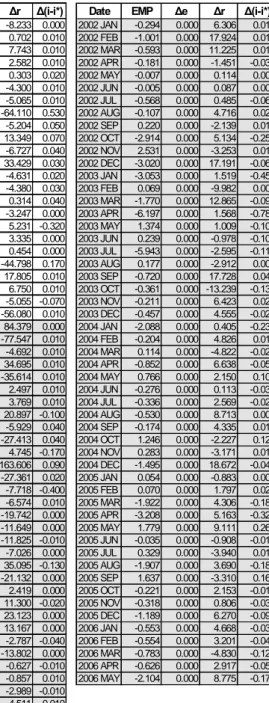
Our estimated measures of EMP for the period January 1992-May 2006 are given in Table 1 and are also depicted graphically in Figure 1. Our first observation is that the monthly EMP values appear to be quantitatively plausible through this period. As is clear from EMP’s descriptive statistics (see Appendix 1), negative EMP is much more prevalent after the change in exchange rate regime in January 1999. Indeed, average EMP for this period is -6.34% p.a. Prior to the peg’s adoption, EMP is generally positive at +8.76% p.a. and, accordingly, the CVE depreciates by 3.35% p.a. on average under that exchange rate regime.
-1 5 -1 0 -5 0 5 10 92 93 94 95 96 97 98 99 00 01 02 03 04 05 06
E MP % E xc ha nge Rate Change
Figure 1
9Using the data for the whole sample period, we calculate the following conversion factors:
Next, we proceed to identify crisis episodes, which we take to refer to an EMP value that exceeds average EMP by one and a half times EMP’s standard devia-tion.10 Under this definition, we find that the EMP measure correctly indicates some known crises periods (e.g. ERM crises, the run-up to, and the wake of, the currency peg’s adoption).11 Other crises episodes, however, need to be further in-vestigated in order to understand the exact nature of the economic and institutional factors that might explain their occurrence. Bubula and Otker-Robe’s (2003) study also sought to identify crises episodes for numerous countries using a similar methodology, including Cape Verde. Based on our results, we found no support for their identification of May 1995 and October 2000 as crises episodes, respec-tively characterised by reserve loss/depreciation and devaluation/reserve loss.
0 1 0 2 0 3 0 4 0 5 0 6 0 7 0 9 2 9 3 9 4 95 9 6 9 7 98 9 9 0 0 01 02 0 3 0 4 05 E MP V ol ati l i ty (% p.a.) Figure 2
10In other words, a crisis episode is characterised by EMP values that satisfy the condition
E M Pt > E M P + 1.5sd, where E M P and sd respectively denote the EMP series’ unconditional
mean and standard deviation.
Table 1 - EMP Estimates & Constituent Components (%)
Date EMP ∆e ∆r ∆(i-i*) Date EMP ∆e ∆r ∆(i-i*) Date EMP ∆e ∆r ∆(i-i*)
1992 JAN 2.437 2.699 4.301 0.000 1997 JAN 5.176 -0.080 -8.233 0.000 2002 JAN -0.294 0.000 6.306 0.010 1992 FEB -0.083 -0.431 -5.714 0.000 1997 FEB -0.577 -0.983 0.702 0.010 2002 FEB -1.001 0.000 17.924 0.010 1992 MAR -0.841 -0.853 -0.198 0.000 1997 MAR 0.466 0.309 7.743 0.010 2002 MAR -0.593 0.000 11.225 0.010 1992 APR -0.632 -0.705 0.277 0.010 1997 APR -4.574 -4.776 2.582 0.010 2002 APR -0.181 0.000 -1.451 -0.030 1992 MAY -0.452 -0.361 1.501 0.000 1997 MAY 4.939 4.688 0.303 0.020 2002 MAY -0.007 0.000 0.114 0.000 1992 JUN -2.408 -2.620 -3.490 0.000 1997 JUN 0.313 -0.128 -4.300 0.010 2002 JUN -0.005 0.000 0.087 0.000 1992 JUL 2.024 2.154 2.130 0.000 1997 JUL 0.969 0.392 -5.065 0.010 2002 JUL -0.568 0.000 0.485 -0.060 1992 AUG -2.071 -0.979 13.513 -0.030 1997 AUG 3.318 -0.941 -64.110 0.530 2002 AUG -0.107 0.000 4.716 0.020 1992 SEP 0.841 0.661 -2.958 0.000 1997 SEP 0.694 0.378 -5.204 0.050 2002 SEP 0.220 0.000 -2.139 0.010
1992 OCT 4.050 3.930 -0.502 0.010 1997 OCT -3.678 0.006 13.349 0.070 2002 OCT -2.914 0.000 5.134 -0.250 1992 NOV -3.240 -3.070 2.802 0.000 1997 NOV 0.623 0.214 -6.727 0.040 2002 NOV 2.531 0.000 -3.253 0.010 1992 DEC -0.213 0.000 3.496 0.000 1997 DEC -1.320 0.714 33.429 0.030 2002 DEC -3.020 0.000 17.191 -0.060
1993 JAN 3.876 4.076 3.280 0.000 1998 JAN 2.685 0.878 -4.631 0.020 2003 JAN -3.053 0.000 1.519 -0.450 1993 FEB 2.180 1.629 -6.099 0.020 1998 FEB -0.720 -1.076 -4.380 0.030 2003 FEB 0.069 0.000 -9.982 0.000 1993 MAR -0.002 -0.376 -0.235 0.040 1998 MAR -0.053 -0.124 0.314 0.040 2003 MAR -1.770 0.000 12.865 -0.090 1993 APR 0.426 0.279 3.484 0.040 1998 APR -0.103 0.327 -3.247 0.000 2003 APR -6.197 0.000 1.568 -0.780 1993 MAY 1.656 0.712 -5.182 0.070 1998 MAY 4.635 4.863 5.231 -0.320 2003 MAY 1.374 0.000 1.009 -0.100
1993 JUN 4.454 3.673 -5.466 0.050 1998 JUN -0.778 -0.575 3.335 0.000 2003 JUN 0.239 0.000 -0.978 -0.100 1993 JUL 1.502 1.048 2.864 0.070 1998 JUL 0.584 0.522 0.454 0.000 2003 JUL -5.943 0.000 -2.595 -0.110 1993 AUG -2.309 -2.767 2.795 0.070 1998 AUG 2.127 -0.688 -44.798 0.170 2003 AUG 0.177 0.000 -2.912 0.000 1993 SEP 2.002 1.030 -5.665 0.070 1998 SEP -0.663 0.330 17.805 0.010 2003 SEP -0.720 0.000 17.728 0.040
1993 OCT 3.852 3.426 4.795 0.080 1998 OCT -0.543 -0.223 6.750 0.010 2003 OCT -0.361 0.000 -13.239 -0.130 1993 NOV 0.064 -1.648 -16.336 0.080 1998 NOV -0.049 -0.446 -5.055 -0.070 2003 NOV -0.211 0.000 6.423 0.020 1993 DEC 0.585 0.073 -5.476 0.020 1998 DEC 3.763 0.262 -56.080 0.010 2003 DEC -0.457 0.000 4.555 -0.020 1994 JAN -0.827 -1.723 -7.353 0.050 1999 JAN -6.244 -0.214 84.379 0.000 2004 JAN -2.088 0.000 0.405 -0.230 1994 FEB -0.607 -0.177 10.006 0.020 1999 FEB 4.952 -0.124 -77.547 0.010 2004 FEB -0.204 0.000 4.826 0.010 1994 MAR 0.494 0.675 5.927 0.020 1999 MAR 0.644 0.000 -4.692 0.010 2004 MAR 0.114 0.000 -4.822 -0.020 1994 APR 1.227 1.006 -2.155 0.010 1999 APR -3.636 0.000 34.695 0.010 2004 APR -0.852 0.000 6.638 -0.050 1994 MAY 0.137 -0.429 -7.834 0.010 1999 MAY 2.974 0.000 -35.614 0.010 2004 MAY 0.766 0.000 2.150 0.100 1994 JUN 1.151 0.300 -11.045 0.020 1999 JUN 0.028 0.000 2.497 0.010 2004 JUN -0.276 0.000 0.113 -0.030 1994 JUL 0.072 -0.254 -5.364 0.000 1999 JUL -3.818 0.000 3.769 0.010 2004 JUL -0.336 0.000 2.569 -0.020 1994 AUG 0.175 -0.575 -10.861 0.010 1999 AUG -1.182 0.000 20.897 -0.100 2004 AUG -0.530 0.000 8.713 0.000 1994 SEP 0.447 0.331 -1.912 0.000 1999 SEP 0.361 0.000 -5.929 0.040 2004 SEP -0.174 0.000 4.335 0.010 1994 OCT 2.367 2.278 -1.460 0.000 1999 OCT 1.668 0.000 -27.413 0.040 2004 OCT 1.246 0.000 -2.227 0.124 1994 NOV 1.407 1.423 0.249 0.000 1999 NOV -0.378 0.000 4.745 -0.170 2004 NOV 0.283 0.000 -3.171 0.010 1994 DEC -0.455 -0.440 0.249 0.000 1999 DEC -9.953 0.000 163.606 0.090 2004 DEC -1.495 0.000 18.672 -0.040
1995 JAN 8.793 -0.276 -0.117 1.010 2000 JAN 0.498 0.000 -27.361 0.020 2005 JAN 0.054 0.000 -0.883 0.000 1995 FEB 0.635 0.645 1.629 0.010 2000 FEB 0.470 0.000 -7.718 -0.400 2005 FEB 0.070 0.000 1.797 0.020 1995 MAR -1.099 -0.844 2.708 -0.010 2000 MAR 0.400 0.000 -6.574 0.010 2005 MAR -1.922 0.000 4.306 -0.185 1995 APR 1.324 1.256 0.365 0.010 2000 APR 1.022 0.000 -19.742 0.000 2005 APR -3.208 0.000 5.163 -0.323 1995 MAY 0.322 0.141 -1.512 0.010 2000 MAY 0.709 0.000 -11.649 0.000 2005 MAY 1.779 0.000 9.111 0.260 1995 JUN -0.592 -1.099 -8.335 0.000 2000 JUN 0.719 0.000 -11.825 -0.010 2005 JUN -0.035 0.000 -0.908 -0.010 1995 JUL 1.084 0.879 -3.363 0.000 2000 JUL 0.069 0.000 -7.026 0.000 2005 JUL 0.329 0.000 -3.940 0.010 1995 AUG 0.162 0.542 6.245 0.000 2000 AUG -2.135 0.000 35.095 -0.130 2005 AUG -1.907 0.000 3.690 -0.188 1995 SEP -1.464 -1.437 1.929 0.010 2000 SEP 1.196 0.000 -21.132 0.000 2005 SEP 1.637 0.000 -3.310 0.160 1995 OCT 2.186 1.764 -6.945 0.000 2000 OCT -0.057 0.000 2.419 0.000 2005 OCT -0.221 0.000 2.153 -0.010 1995 NOV 1.498 1.644 2.402 0.000 2000 NOV -0.777 0.000 11.300 -0.020 2005 NOV -0.318 0.000 0.806 -0.030 1995 DEC -0.367 -0.953 -8.162 0.010 2000 DEC -1.317 0.000 23.123 0.000 2005 DEC -1.189 0.000 6.270 -0.090 1996 JAN 3.205 0.085 -51.300 0.000 2001 JAN -0.891 0.000 13.167 0.000 2006 JAN -0.553 0.000 4.668 -0.030 1996 FEB 1.760 0.216 -25.378 0.000 2001 FEB 0.259 0.000 -2.787 -0.040 2006 FEB -0.554 0.000 3.201 -0.040
1996 MAR 3.860 1.201 -42.249 0.010 2001 MAR 0.929 0.000 -13.802 0.000 2006 MAR -0.783 0.000 -4.830 -0.120 1996 APR 0.510 0.929 5.415 -0.010 2001 APR 1.922 0.000 -0.627 -0.010 2006 APR -0.626 0.000 2.917 -0.050 1996 MAY -0.902 -0.219 12.706 0.010 2001 MAY -0.038 0.000 -0.857 0.010 2006 MAY -2.104 0.000 8.775 -0.175 1996 JUN 1.039 1.183 2.367 0.000 2001 JUN 0.451 0.000 -2.989 -0.010 1996 JUL 1.922 0.123 -28.094 0.010 2001 JUL 3.404 0.000 4.511 0.010 1996 AUG 0.390 0.653 5.792 0.010 2001 AUG 0.005 0.000 2.871 -0.010 1996 SEP -2.239 -0.902 23.454 0.010 2001 SEP -0.096 0.000 4.532 0.010 1996 OCT 1.049 0.313 -9.154 0.020 2001 OCT -0.283 0.000 7.594 0.010 1996 NOV 0.330 -0.177 -6.853 0.010 2001 NOV 0.264 0.000 0.078 0.210 1996 DEC -3.856 1.173 84.154 0.010 2001 DEC -1.908 0.000 35.783 -0.010
We find that the pre-peg period witnessed ten crisis episodes, all associated with positive EMP pressures, whilst only two occurred afterward. This finding suggests that two distinct EMP states might be present over our sample period, each characterised by a different volatility level. To see if this is the case, we calculate the mean annual EMP-volatility using the (unconditional) standard de-viation of the monthly EMP values.
As can be seen in Figure 2, we observe that EMP volatility has declined dra-matically since 1999, during which it peaked at 61.4%. Moreover, volatility has remained low and relatively stable over the period 2000-2005, averaging 9.44% p.a.. In contrast, volatility averages 20.35% p.a. for the remaining period. This last observation clearly points to a secular change of EMP dynamics during 1999, which clearly needs to be further explored. In the next section, therefore, we study the stochastic properties of EMP’s conditional mean and variance so as to better understand the behaviour of Cape Verde’s exchange rate arrangements over time.
3
Econometric Analysis
3.1
Model Specification
Following Braga de Macedo et al. (2004a, 2006) and Brites Pereira (2005a), we propose an E G A RC H( p, q) process for the conditional variance equation in order to capture possible heteroskedasticity effects, volatility clustering and leverage effects associated with asymmetric responses shocks:
t = σtzt zt ∼ Dϑ(0, 1) lnσ2t = λst+ p ; j =1 βjlnσ2t− j+ q ; i =1 t αi n n n nσt−it−i n n n n + γi t−i σt−i u
where t is the mean EMP equation’s disturbance term, assumed to have a zero mean and to be serially uncorrelated, while Dϑ(0, 1) is a probability density func-tion with zero mean and unit variance.12 Moreover, stis an r ×1 vector of explana-tory variables, including a constant term, andλ is the respective 1 × r coefficient 12Optionally,ϑ are additional distributional parameters that can be used to describe a
distribu-tion’s skew and shape. For a full discussion of this class of models, refer to Engle (1982) and Bollerslev (1986).
vector. Note that the left-hand side above is the logarithm of the conditional vari-ance, which implies that the associated leverage effect is exponential rather than quadratic. In addition, forecasts of the conditional variance are guaranteed to be non-negative under this specification.
As for the mean EMP equation, we follow Engle, Lilien & Robins (1987) in allowing mean EMP to depend on its own conditional variance. This captures the basic insight that risk-averse agents will require compensation for holding a risky asset. Given that an asset’s riskiness can be measured by the variance of returns, the risk premium is an increasing function of the returns’ conditional variance. For exchange rates, the risk premium associated with the underlying volatility can be either positive or negative.13
In the context of EMP, the risk-return relationship implies that holding assets of a country in which EMP-volatility is high (largeσ2
t) should be compensated by a greater return (lower EMP). This implies thatµ < 0 in our specification of the mean EMP equation, given below:
E M Pt = µ ln σ2t + θ xt+ m ; i =1 ξiE M Pt−i + n ; j =1 ψj t− j + t
which also incorporates the effect of economic fundamentals. Their impact is captured by the k ×1 vector of explanatory variables xt (includes a constant term), withθ being the respective 1 × k coefficient vector. All explanatory variables are lagged one period in order to avoid the problem of contemporaneous simultaneity with the dependent variable. We also allow for A R M A(m, n) terms in our mean equation given our lack of data pertaining to economic fundamentals for part of our sample.
For the full sample period, we estimate the above “EGARCH in the Mean” (EGARCH-M) model which additionally incorporates a dummy variable that cap-tures the CVE’s change in exchange rate regime. As such, the dummy takes on the value one ∀t ≥1999:01 and zero otherwise. Our choice of economic funda-mentals is based on the relevant theoretical and empirical literature, as discussed 13As Engel (1996) shows, the direction of the effect of conditional variance on risk premiums
depends on the variance of nominal consumption. Fukuta & Saito (2002) show that the signs of the coefficients on risk premiums depend on the covariance between consumption growth and inflation, the intertemporal marginal rate of substitution, and the variances of inflation in Japan and the United States.
in Flood and Marion (1998). For Cape Verde, however, our choice is severely restricted by the lack of data pertaining to some of these fundamentals. At best, the data are available but have a low trimesterly or annual frequency. At worst, the data simply do not exist, as is especially true prior to January 1999.
In practice, we were able to choose four fundamentals for the mean equation that had the desired monthly frequency (see Appendix 3 for the data’s description): domestic credit growth rate( dct), real depreciation rate (qt), government bor-rowing growth rate( gvtt) and the change in emigrant’s remittances ( remt).14 The choice of the last variable is justified primarily by the importance that emi-grant’s remittances have in the Cape Verdian economy, as discussed above. More-over, it is the only element of Cape Verde’s current account that can be included in our analysis, given the monthly frequency of the data. In the conditional variance equation, we include foreign reserve changes( rt) given their important role in EMP dynamics under the currency peg.15
Turning to the expected signs of these other variables, domestic credit growth and increased government borrowing necessarily lead to greater EMP, implying that the estimated coefficients are expected to be positive. On the other hand, increased external transfers and real depreciation lead to lower EMP, hence the expected signs are negative. As for conditional variance, while the expected sign of the (lagged) explanatory variables is not easily predictable a priori on theo-retical grounds, their effects are easily interpretable upon estimation. In the case of foreign reserves, for example, a negative coefficient indicates that an increase in foreign reserves lowers conditional volatility. Finally, the impact of shocks is asymmetric if γ = 0 while the presence of leverage effects can be tested by the hypothesis that γ < 0, i.e. negative shocks increase conditional volatility more than positive shocks, as is to be expected under the normal functioning of markets.
3.2
Estimation Results
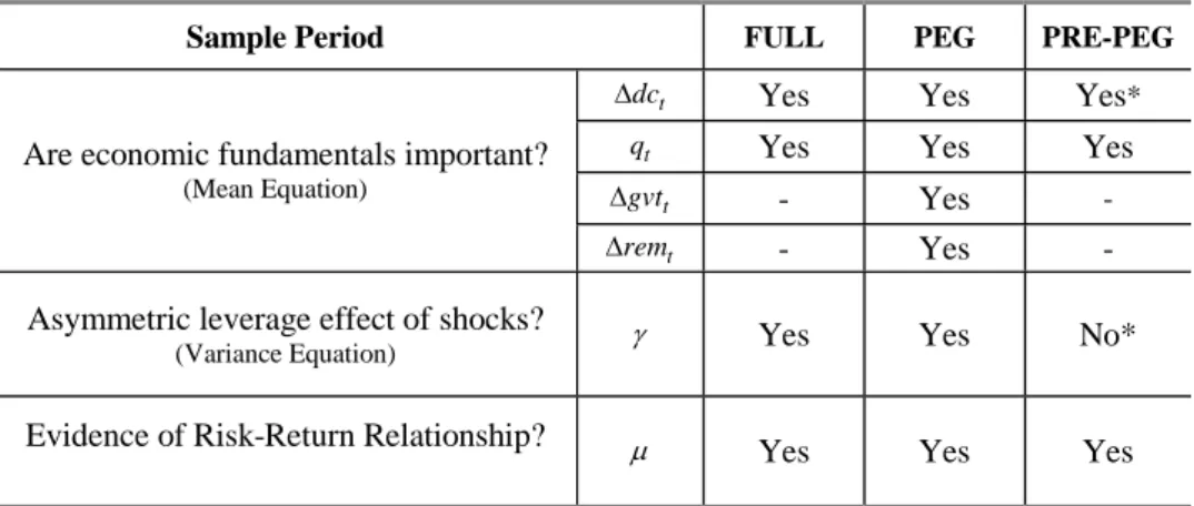
The empirical analysis is undertaken using monthly data for the period January 1992-May 2006. We first estimate an EGARCH-M model for the full sample period using domestic credit growth, real depreciation and the regime dummy
14The data pertaining to the latter three variables are available only as of January 1999. 15Note that changes in reserves and in the interest rate differential are not included in the mean
as explanatory variables. The summary of this estimation’s results, as that of subsequent ones, is given in Table 2.
Table 2 - Summary of EGARCH-M Estimation Results
Sample Period FULL PEG PRE-PEG
t
dc
∆ Yes Yes Yes*
t
q Yes Yes Yes
t
gvt
∆ - Yes -
Are economic fundamentals important?
(Mean Equation)
t
rem
∆ - Yes -
Asymmetric leverage effect of shocks?
(Variance Equation) γ Yes Yes No*
Evidence of Risk-Return Relationship? µ Yes
Yes Yes
Notes: *Refer to the comment of footnote 16. For the estimation procedure and results, see Appendix 2.
We find economic fundamentals to be important, as expected. In addition, there is evidence of the risk-return relationship and of an asymmetric leverage effect of shocks on the conditional variance. Significantly, we find that the change in exchange rate regime also explains EMP dynamics over the sample period, and is associated with a reduction of mean EMP and of volatility.
This last result reinforces our earlier finding that two distinct EMP regimes might be present over the sample period. With this mind, we gain additional insight by dividing the sample into two sub-samples, associated with the “pre-” and “post-“pre-” currency peg arrangement. Although data availability hampers an effective comparison of these two periods, it is nonetheless clear after looking at the estimation results that fundamentals account for EMP’s behaviour better under the currency peg.
Prior to the regime change, changes in domestic credit growth and in the real exchange rate affect mean EMP and do not affect the conditional variance.16 As was also the case under the full sample, volatility is driven essentially by changes 16Compared to the results obtained under a currency peg and the full sample, however, it would
in foreign exchange reserves. However, now there is no evidence of negative shocks affecting volatility differently, which also contrasts with the result obtained under the currency peg. The estimate of the risk-return relationship for “pre-peg” period implies that a 1% increase in monthly volatility is associated with a reduction of 0.52% in mean EMP, or equivalently 6.26% p.a.17
Under the currency peg, increases in domestic credit and government debt lead, as expected, to greater EMP. The same holds true for a decline in emigrant’s remittances and for a real exchange rate appreciation. Conditional volatility re-mains driven by foreign reserve changes and negative shocks affect volatility dif-ferently than do positive shocks. We again find that an increase in monthly volatil-ity leads to lower EMP but the risk-return relationship is such that a 1% increase in monthly volatility leads to smaller reduction of mean EMP - almost half of that found for the “pre-peg” period given our estimated return of 0.25%.
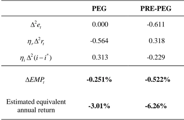
The expected return from holding assets from Cape Verde under the currency peg is thus lower for the same increase in volatility. We explain this finding af-ter assessing how the three channels for the relief of EMP operate across the two regimes. In other words, we seek to decompose the change in EMP into the under-lying changes of its constituent elements in order to see how these are relieving, or not, prevailing EMP.18The result of this decomposition is shown in Table 3.
17To see this, note that the derivative of mean EMP with respect toσ2
t yields the semi-elasticity
of changes in EMP for a given percentage change in variability(d E M Pt
dσ2
t/σ2t = µ), ceteris paribus.
Assuming discrete monthly changes, the latter expression can be rewritten as E M Pt = µ σ
2
t
σ2
t
so as to highlight the risk-return relation. When variability increases by 1%, EMP must decrease byµ% in order for this relation to hold.
18To undertake this task, we define the change in EMP as
E M Pt = 2et+ ηr 2rt + ηi 2(it− it∗)
where 2denotes the second difference operator. We then rewrite the above expression as
E M Pt = et v 2e t et w + ηr rt v 2r t rt w + ηi (it − it∗) v 2(i t − it∗) (it− it∗) w
in order to estimate the three expressions given by the square brackets, which are interpretable as the rate of acceleration of the changes in et, rt and(it− i∗t) respectively. Estimation is possible
as there is one equation for each of the three sample periods considered. Moreover, the system of equations is identifiable as there exists an unique value for E M Pt and also unique mean
values for et, rt and (it − it∗) for each sample period. Upon estimation, we find that 2e
t
Table 3 - Decomposition of EMP Return (%) PEG PRE-PEG t e 2 ∆ 0.000 -0.611 t r r 2 ∆ η -0.564 0.318 ) ( * 2 i i i∆ − η 0.313 -0.229 t EMP ∆ -0.251% -0.522% Estimated equivalent annual return -3.01% -6.26%
Notes: Recall that EMP 2e 2r 2(i i*)
i t r t
t =∆ + ∆ + ∆ −
∆ η η . For each regime, the
above terms are calculated using the mean values of ∆ ,et∆rt and ∆(i−i*), as discussed in footnote 18.
Prior to the peg’s adoption, we know that the CVE was depreciating and that the interest rate differential was increasing, both at a decelerating rate based on our calculations, while foreign reserves were declining at an accelerating rate, as can be seen in Figure 3. As a result, the foreign reserves channel is associated with a positive monthly change in EMP, which represents a loss on holding Cape Verdian assets estimated to be 0.32%. The opposite is true, meanwhile, for the other two channels and, as is clear from Table 3, the net effect implies a negative change in EMP (positive return) for the “pre-peg” period.
Note, however, that this return is largely due to the exchange rate channel, i.e. a slowing CVE depreciation rate, hence the increasing economic benefit associ-ated with holding assets denominassoci-ated in CVE. Indeed, once this channel’s effect is netted out, the combined impact of the remaining channels actually implies an expected annual loss of 1.07% on holding such assets. In contrast, the interest rate differential was decreasing at an accelerating rate while foreign reserves were increasing at a decelerating rate during the “peg” period. Here, the foreign re-serves channel is associated with a positive return while the interest rate channel’s contribution is negative given the lower interest rate differential (see Figure 3).
−2.72%, 2r t rt = 2.54% and 2(i t−it∗)
(it−it∗) = −1.02%, which allows us to decompose E M P into
80 85 90 95 100 105 110 115 92 94 96 98 00 02 04 06
CVE/EURO Exchange Rate 0 50 100 150 200 250 92 94 96 98 00 02 04 06
Foreign Reserves (million USD)
0 1 2 3 4 92 94 96 98 00 02 04 06
Interest Rate Differential (%)
-6 -4 -2 0 2 4 6 92 94 96 98 00 02 04 06
% Exchange Rate Change
-100 -50 0 50 100 150 200 92 94 96 98 00 02 04 06
% Foreign Reserves Change
-1.0 -0.5 0.0 0.5 1.0 1.5 92 94 96 98 00 02 04 06
% Interest Differential Change
Figure 3
The composition of the expected return under the currency peg is “more vir-tuous” in that is it not due either to a larger risk premium, as measured by the interest rate differential, nor favourable exchange rate movements. Rather, it is due to the strengthening of Cape Verde’s foreign reserve position, which we take to be a sign of the credibility of its currency peg, especially as Cape Verde’s for-eign reserves are particularly sensitive to external and fiscal factors, as discussed in Weber (2005). This last finding is reinforced by the fact that we also find ev-idence of the asymmetric leverage effect of shocks where the influence of “bad EMP news” outweighs that of “good EMP news”, as is to be expected under in-creased market scrutiny.
4
Conclusion
This paper seeks to infer the credibility of Cape Verde’s interaction between ex-change rate, economic policy regime and financial-market integration. In doing so, we continue the line of research that previously studied the cases of Portu-gal’s Escudo and Macau’s Pataca. The former currency disappeared and the latter has an unique double peg under a currency board, in which the nature of EMP
changes in a fundamental way. For Cape Verde, we were able to ascertain the credibility of its currency peg to the Euro by analysing the impact of economic fundamentals, our explanatory variables, on the stochastic properties of EMP, the dependent variable, using EGARCH-M models. We measure EMP as a weighted linear combination of changes in the exchange rate, in foreign exchange reserves and in the interest rate differential.
Our initial descriptive analysis of EMP finds a substantial reduction in the number of crisis episodes and of (unconditional) volatility after the currency peg’s adoption. Moreover, our subsequent EGARCH-M estimation results suggest that mean EMP is driven by the usual economic fundamentals and that conditional variability is more sensitive to “bad EMP news” than to “good EMP news”. We also find evidence that the expected return from holding assets from Cape Verde under the currency peg is lower for the same increase in volatility.
We explain this finding by the fact that the composition of the expected return under the currency peg is “more virtuous” in that is it not due to either a larger risk premium nor favourable exchange rate movements. Rather, it is due to the strengthening of Cape Verde’s foreign reserve position, which we take to be a sign of the credibility of its currency peg. Our view is further reinforced if one bears in mind that there has been a strong and gradual build-up of foreign reserves since 2001, partly as a result of the Cape Verdian government’s formal recognition of the need to consolidate monetary and fiscal policy through the adoption of the Maastricht criteria as reference values.
In other words, Cape Verde has “got it right” when it comes to its currency peg, as the peg apparently reflects the intertemporal credibility of Cape Verdian economic policy and so has successfully withstood the scrutiny of international markets. Needless to say, our finding needs to be further tested given that our analysis is based on an ad-hoc EMP measure, which implies some degree of cau-tion when interpreting our estimates. This task will also be greatly facilitated by the availability of more detailed data of higher frequency and more sophisticated modelling techniques. Until then, we would like to compare the operation of the Cape Verdian and the Pataca pegs, by using the latter specification insofar as we have monetary data with sufficiently high frequency.
Our agenda for deepening and widening this research seeks to support Cape Verde’s development strategy as a CPLP country that is graduating from aid-dependence and whose political governance has been praised by the international
community.19 In addition, Cape Verde may decide to increase its trading in inter-national financial and capital markets in the future. Deepening the analysis thus involves investigating the costs and benefits of adopting the Euro at some point in the future, a decision that requires an understanding of prevailing currency peg’s credibility. On the other hand, broadening the analysis leads to comparisons with other CPLP countries and Macau.
We will also turn our attention to the operation of exchange rate regimes in other Lusophone countries, such as those of Mozambique and São Tomé e Principe, where similar EMP variables could be calculated with the available data and compare their managed floating to the Cape Verdian experience. In doing so, we hope to provide evidence on the benefits of greater mutual knowledge among not just CPLP member countries but also between these and the various economic regimes present in China.
19Braga de Macedo, Braz and Mantero (2003) present the implications of the Monterrey
consen-sus for CPLP and emphasize the role of public-private partnerships as a means to promote better policies. Macau has been active in seeking cooperation with CPLP since the Ministerial con-ference of October 2003, where, significantly, the OECD experience with peer-pressure was dis-cussed. The fact that the Chinese authorities have established the secretariat of the sino-lusophone economic partnership forum in Macau might encourage further comparative studies along these lines.
5
References
Bollerslev, T. (1986) “Generalized Autoregressive Conditional Heteroscedas-ticity”, Journal of Econometrics, No. 31, pp. 307-27.
Bollerslev, T. and J. Wooldridge (1992) “Quasi-Maximum Likelihood Estima-tion and Inference in Dynamic Models with Time Varying Covariances”, Econo-metric Reviews, No. 11, pp. 143-172.
Bonaglia, F., Braga de Macedo, J. and M. Bussolo (2001) “How Globalisation Improves Governance”, CEPR Discussion Paper, No. 2992, October.
Braga de Macedo, J., Eichengreen B. and J. Reis (1996) editors Currency Convertibility: The Gold Standard and Beyond, London: Routledge.
Braga de Macedo, J. (2001a) “Crises? What Crises? Escudo from ECU to EMU”, in Short-Term Capital Flows and Economic Crises, edited by Stephany Griffith-Jones, Manuel Montes and Anwar Nasution, study prepared for UNU/ WIDER, Oxford University Press, pp.253-260.
Braga de Macedo, J., Cohen, D. and H. Reisen (2001b), editors, Don’t Fix Don’t Float, Paris: OECD Development Centre.
Braga de Macedo, J. and B. Eichengreen (2001c) “The European Payments Union and its Implications for the Evolution of the International Financial Ar-chitecture”, in Fragility of the International Financial System - How Can We Pre-vent New Crises in Emerging Markets?, edited by Alexandre Lamfalussy, Bernard Snoy and Jérôme Wilson, Brussels: PIE Peter Lang for Fondation Internationale Robert Triffin, pp. 25-42.
Braga de Macedo, J., Nunes, L. C. and L. Brites Pereira (2003) “Central Bank Intervention Under Target Zones: The Portuguese Escudo in the ERM”, FEUNL Working Paper, No. 345, Lisbon: Universidade Nova de Lisboa.
Braga de Macedo, J., Catela Nunes, L. and F. Covas (2004a) “Moving the Escudo into the Euro” in chapter 8 of Shaping the New Europe: Economic Pol-icy Challenges of EU Enlargement, edited by Michael Landersmann and Darius Rosati, Palgrave, forthcoming (an earlier version appeared as CEPR Discussion Paper, No. 2248, October 1999).
Braga de Macedo, J. and H. Reisen (2004b), “Float in Order to Fix: Lessons from Emerging Markets for New EU Member Countries”, in Monetary Strategies for Joining the Euro, National Bank of Hungary, pp. 109-113.
Braga de Macedo, J. and M. Grandes (2005) “Argentina and Brazil Risk: a Eurocentric Tale”, in Rolf Langhammer e Lucio Vinhas de Souza, editors Mone-tary Policy and Macroeconomic Stabilization in Latin America, Berlin: Springer, pp. 153-172.
Braga de Macedo, J., Braz, J., Brites Pereira, L. and L. C. Nunes (2006) Re-port to the Monetary Authority of Macau on “Macau’s Currency Board”, FEUNL Working Paper, No. 492, Lisbon: Universidade Nova de Lisboa.
Braga de Macedo, J. and J. Oliveira Martins (2006) “Growth, Reform Indi-cators and Policy Complementaries,, FEUNL Working Paper, No. 484, Lisbon: Universidade Nova de Lisboa.
Brites Pereira (2005a), “The Effectiveness of Intervention: Evidence from a Markov-Switching Analysis”, Manuscript, Doctoral Thesis, Lisbon: Univer-sidade Nova de Lisboa.
Brites Pereira (2005b), “Relieving Exchange Market Pressure”, Manuscript, Doctoral Thesis, Lisbon: Universidade Nova de Lisboa.
Bubula, A. and I. Otker-Robe (2006) “Are Pegged and Intermediate Exchange Rate Regimes More Crisis Prone?, IMF Working Paper, No. 03/223, Washington: International Monetary Fund.
Dooley, M. D. Folkerts-Landau and P. Garber (2005) “Interest rates, Exchange Rates and International Adjustment”, NBER Working Paper.
Engel, C., (1996), “The Forward Discount Anomaly and the Risk Premium: A Survey of Recent Evidence”, Journal of Empirical Finance, No. 3, pp.123-192.
Engle, R. (1982) “Autoregressive Conditional Heteroscedasticity with Esti-mates of the Variance of United Kingdom Inflation”, Econometrica, No. 50, pp. 987-1007.
Engle, R., Lilien, D. and R. Robins (1987) “Estimating Time Varying Risk Premia in the Term Structure: The ARCH-M Model”, Econometrica, No. 55, pp. 391-407.
Eichengreen, B., Rose, A. K. and C. Wyplosz (1995) “Exchange Market May-hem: The Antecedents and Aftermath of Speculative Attacks”, Economic Policy, Vol. 21, pp. 249-312.
Eichengreen, B., Rose, A. K. and C. Wyplosz (1996) “Speculative Attacks on Pegged Exchange Rates: An Empirical Exploration with Special Reference to the European Monetary System”, in Canzoneri, M.B., Ethier W.J. and V. Grilli (eds.) The New Transatlantic Economy, Cambridge University Press, Cambridge.
Flood, R. and N. Marion (1998) “Perspectives on Recent Currency Crisis Lit-erature”, NBER Working Paper, No. 6380, Cambridge, MA: National Bureau of Economic Research.
Fukuta, Y. and M. Saito (2002) “Forward Discount Puzzle and Liquidity Ef-fects: Some Evidence from Exchange Rates among the United States, Canada, and Japan”, Journal of Money, Credit and Banking, Vol.34, pp. 1014-1033.
Girton, L. and D. Roper (1977) “A Monetary Model of Exchange Market Pres-sure Applied to the Postwar Canadian Experience”, American Economic Review, Vol. 67, No. 4, pp. 537-548.
Goldberg, L. and M. Klein (2006) “Establishing Credibility: Evolving Per-ceptions of the European Central Bank”, paper presented at the NBER Summer Institute, July.
Kose, M., Prasad, E., Wei, S. and K. Rogoff (2006) “Financial Globaliza-tion: A Reappraisal”, IMF Working Paper, No. 06/189, Washington: International Monetary Fund.
Kouri, P. and J. Braga de Macedo (1978) “Exchange Rates and the Interna-tional Adjustment Process”, Brookings Papers on Economic Activity.
Krugman, P. (1981) “Oil and the Dollar”, in J. Bhandari and J. Putnam, Inter-dependence under Flexible Exchange Rates, Cambridge: MIT
Schuler, K. (2004) Tables of Modern Monetary History, http://users.erols.com/ kurrency/afrca.htm
Spolander, M. (1999) “Measuring Exchange Rate Pressure and Central Bank Intervention”, Bank of Finland Studies, Series E, No. 17.
Weber, R. (2005) “Cape Verde’s Exchange Rate Policy and its Alternatives”, BCL Working Paper, No. 16, Banque Central du Luxembourg.
Weymark, D. N. (1995) “Estimating Exchange Market Pressure and the De-gree of Exchange Market Intervention for Canada”, Journal of International Eco-nomics, Vol. 39, pp. 273-295.
Weymark, D. N. (1998) “A General Approach to Measuring Exchange Market Pressure”, Oxford Economic Papers, Vol. 50, pp. 106-121.
Appendix 1
EMP Descriptive Statistics
0 4 8 1 2 1 6 - 4 - 2 0 2 4 6 8 Series: EMP Sample 1992:01 1998:12 Observations 84 Mean 0.715476 Median 0.460000 Maximum 8.790000 Minimum -4.570000 Std. Dev. 2.153844 Skewness 0.570363 Kurtosis 4.701327 Jarque-Bera 14.68519 Probability 0.000647 0 5 1 0 1 5 2 0 2 5 * - 8 - 6 - 4 - 2 0 2 4 Series: EMP Sample 1999:01 2006:05 Observations 89 Mean -0.513146 Median -0.180000 Maximum 4.950000 Minimum -9.950000 Std. Dev. 2.047069 Skewness -1.529094 Kurtosis 8.416259 Jarque-Bera 143.4694 Probability 0.000000
Appendix 2
EGARCH-M Estimation Results
In the estimation of the our EGARCH-M models, we started with a general specification of the mean and variance equations. The orders of the variance equa-tion and ARMA process in the mean equaequa-tion were determined by the partial au-tocorrelation and the auau-tocorrelation function of the EMP series. Non-significant variables are excluded from an estimated equation whenever appropriate. We use the Schwartz Information Criterion (SIC) to assess a model’s relative fit, implying that we choose those models for which the (negative) SIC is smallest. The final EGARCH-M specifications were decided by looking at the properties of standard-ised residuals (SR) and squared standardstandard-ised residuals (SSR).
The models were estimated using E-Views 3.0, and we employed the Mar-quardt nonlinear optimization algorithm to compute maximum likelihood param-eters. Bollerslev and Wooldridge (1992) note that maximising a mis-specified likelihood function in a GARCH framework provides consistent parameter esti-mates, though the standard errors will be understated. Accordingly, we use their consistent variance-covariance estimator to correct the covariance matrix. We thus report asymptotic standard errors for the estimated parameters that are robust to departures from normality.
Correctly specified EGARCH-M models will have SR and SSR that are white noise, i.e. they are independent and identically distributed random variables with mean zero and variance one.20 As model diagnostic tools, we use the modified Box-Ljung (B-L) procedure on the SR series to test for remaining serial corre-lation in the mean equation. To detect remaining ARCH effects in the variance equation, we use the B-L test as well as the ARCH-LM test on SSR. Based on the results of the diagnostic tests, we find ample support for our model specifica-tion. The B-L Q-statistics are insignificant at the 5% level for both the mean and variance equation, as are those of the ARCH-LM test.
20If the standardised residuals are also normally distributed, then the estimates are maximum
likelihood estimates which are asymptotically efficient. However, even if the residual’s distribution is not normal, the estimates are still consistent under quasi-maximum likelihood assumptions.
Table A2.1 - FULL Sample Period: 1992:01 2006:05
Mean: EMPt =µ σ + +θ0+θ1∆dct−3+θ2qt−7+ξ1EMPt−1+εt
2
DUMMY ln
Parameter Estimate Std. Error t-Statistic p-value
µ -8.509144 3.292073 -2.584737 0.0097** DUMMY -0.009118 0.002093 -4.356396 0.0000** θ0 0.009435 0.002264 4.167470 0.0000** 1 θ 0.151282 0.031037 4.874198 0.0000** 2 θ -0.177364 0.043724 -4.056472 0.0000** 1 ξ -0.145674 0.049092 -2.967362 0.0030** Variance: 1 1 1 1 1 1 9 3 3 2 2 1 0 2 DUMMY ln − − − − − − − + ∆ + ∆ + + ∆ + + = t t t t t t t t r r r σ ε γ σ ε α λ λ λ λ σ DUMMY -0.699251 0.338118 -2.068065 0.0386* 0 λ -7.750207 0.260143 -29.79215 0.0000** 1 λ -5.151746 0.470296 -10.95426 0.0000** 2 λ -1.252714 0.394093 -3.178730 0.0015** 3 λ -1.569033 0.331614 -4.731500 0.0000** 1 α 0.012708 0.176261 0.072099 0.9425 1 γ -0.323115 0.117119 -2.758871 0.0058** Diagnostics Ljung-Box Standardised Residuals Ljung-Box Squared Residuals ARCH-LM Statistic
Lag Q p-value Q2 p-value LM p-value
Lag1 1.5695 0.210 0.4417 0.506 0.015103 0.7444 Lag2 4.1114 0.128 0.4770 0.788 -0.077877 0.1312 Lag3 6.1143 0.106 0.6834 0.877 -0.011084 0.8917 Lag4 6.3763 0.173 0.8711 0.929 -0.016844 0.7653 Lag5 6.4248 0.267 1.1180 0.952 -0.039866 0.3550 Lag6 7.2954 0.294 1.6650 0.948 -0.021707 0.7914 Lag7 7.3028 0.398 1.7521 0.972 -0.076957 0.1113 Lag8 7.3255 0.502 2.7290 0.950 -0.030174 0.5162 Lag9 7.6434 0.570 3.4612 0.943 -0.095946 0.0712 Lag10 9.4747 0.488 5.1373 0.882 -0.066391 0.1363 Lag11 11.337 0.415 5.3151 0.915 0.072194 0.5766 Lag12 1.5695 0.210 0.4417 0.506 -0.049595 0.2651
No. of Observations Log-Likelihood SIC
163 430.8775 -4.8806
Notes: The parameters are as defined in the main text. A double (single) asterisk indicates that the estimated parameter is significantly different from zero at the 1% (5%) level.
Table A2.2 - PEG Sample Period: 1999:01 2006:05
Mean: EMPt=µ σ +θ0+θ1∆dct−3+θ2qt−2+θ3∆gvtt−1+θ4∆remt−2+ξ2EMPt−2+εt 2
ln
Parameter Estimate Std. Error t-Statistic p-value
µ -25.07902 6.883798 -3.643195 0.0003** θ0 -0.000018 0.001614 -6.293150 0.5542 1 θ 0.126127 0.011710 10.77061 0.0000** 2 θ -0.201724 0.040910 -4.930950 0.0000** 3 θ 0.082055 0.007732 10.61264 0.0000** 4 θ -0.010158 0.001614 -6.293150 0.0000** 2 ξ -0.044702 0.006064 -7.371781 0.0000** Variance: 1 1 1 1 1 1 9 3 3 2 2 1 0 2 ln − − − − − − − + ∆ + ∆ + + ∆ + = t t t t t t t t r r r σ ε γ σ ε α λ λ λ λ σ 0 λ -8.001452 0.244823 -32.68260 0.0000** 1 λ -7.230037 0.541340 -13.35581 0.0000** 2 λ -2.297204 0.696531 -3.298062 0.0010** 3 λ -2.194838 0.359837 -6.099539 0.0000** 1 α -1.093911 0.224641 -4.869594 0.0000** 1 γ -0.949438 0.181944 -5.218294 0.0000** Diagnostics Ljung-Box Standardised Residuals Ljung-Box Squared Residuals ARCH-LM Statistic
Lag Q p-value Q2 p-value LM p-value
Lag1 0.7889 0.374 0.1353 0.713 0.156352 0.1872 Lag2 0.7932 0.673 0.7789 0.677 -0.138131 0.2717 Lag3 0.9269 0.819 0.7797 0.854 0.223788 0.2957 Lag4 0.9270 0.921 1.0320 0.905 -0.109044 0.3381 Lag5 1.1182 0.952 1.4195 0.922 0.179680 0.1127 Lag6 1.1485 0.979 1.4714 0.961 -0.184948 0.0590 Lag7 1.2944 0.989 1.8006 0.970 0.067827 0.7225 Lag8 1.3134 0.995 2.0008 0.981 -0.028805 0.8148 Lag9 1.3140 0.998 2.0259 0.991 0.001195 0.9415 Lag10 2.0649 0.996 2.0262 0.996 -0.015050 0.4470 Lag11 2.2970 0.997 2.1063 0.998 0.003805 0.8222 Lag12 2.4421 0.998 2.1067 0.999 -0.017295 0.1169
No. of Observations Log-Likelihood SIC
84 258.1291 -5.5657
Notes: The parameters are as defined in the main text. A double (single) asterisk indicates that the estimated parameter is significantly different from zero at the 1% (5%) level.
Table A2.3 - PRE-PEG Sample Period: 1992:01 1998:12
Mean: EMPt=µ σ +θ0+θ1∆dct−2+θ2qt−3+ξ1EMPt−1+ξ2EMPt−2+ξ3EMPt−3+ψ1εt−1+ψ2εt−2+εt 2
ln
Parameter Estimate Std. Error t-Statistic p-value
µ -52.23944 23.61302 -2.212315 0.0269* θ0 0.029649 0.005884 5.038987 0.0000** 1 θ -0.211114 0.054662 -3.862177 0.0001** 2 θ -0.206451 0.057801 -3.571741 0.0004** 1 ξ -0.320130 0.050626 -6.323459 0.0000** 2 ξ -0.840518 0.024433 -34.40028 0.0000** 3 ξ -0.283066 0.041766 -6.777481 0.0000** 1 ψ -0.098286 0.024881 -3.950292 0.0001** 2 ψ 0.954739 0.022616 42.21508 0.0000** Variance: 1 1 1 1 1 1 9 3 3 2 2 1 0 2 ln − − − − − − − + ∆ + ∆ + + ∆ + = t t t t t t t t r r r σ ε γ σ ε α λ λ λ λ σ 0 λ -7.671796 0.315678 -24.30258 0.0000** 1 λ -0.985628 0.387202 -2.545513 0.0109* 2 λ 0.684963 0.501770 1.365093 0.1722 3 λ -1.407724 0.517449 -2.720507 0.0065** 1 α -0.641733 0.244187 -2.628036 0.0086** 1 γ 0.043852 0.104720 0.418753 0.6754 Diagnostics Ljung-Box Standardised Residuals Ljung-Box Squared Residuals ARCH-LM Statistic
Lag Q p-value Q2 p-value LM p-value
Lag1 2.4366 0.119 0.0736 0.786 0.003201 0.8983 Lag2 2.5308 0.282 0.0930 0.955 -0.017088 0.4878 Lag3 2.5674 0.463 0.1137 0.990 -0.010469 0.5020 Lag4 2.5739 0.631 0.1329 0.998 -0.086750 0.4395 Lag5 2.5827 0.764 0.1516 1.000 0.008703 0.7758 Lag6 2.6127 0.856 0.1695 1.000 -0.063620 0.4549 Lag7 2.6149 0.918 0.1928 1.000 -0.096782 0.4270 Lag8 2.6149 0.956 0.2150 1.000 -0.008545 0.5186 Lag9 2.6214 0.977 0.2157 1.000 -0.008222 0.4471 Lag10 2.6214 0.989 0.2165 1.000 -0.018768 0.4171 Lag11 2.6318 0.995 0.2172 1.000 -0.057575 0.4622 Lag12 2.4366 0.119 0.2179 1.000 -0.399223 0.4518
No. of Observations Log-Likelihood SIC
79 210.4824 -4.4990
Notes: The parameters are as defined in the main text. A double (single) asterisk indicates that the estimated parameter is significantly different from zero at the 1% (5%) level.
Appendix 3 Data Description
The data used in the analysis are monthly and the sample period runs from Jan-uary 1992 until May 2006. Some series, however, are unavailable with a monthly frequency prior to January 1999, as detailed in the main text. Where appropriate, changes between two consecutive months, denoted by the symbol, are calcu-lated as the natural log difference of the variables in question, with the exception of interest rates.
et- Bilateral CVE/Euro exchange rate. Source: Banco de Cabo Verde (BCV).21 et - Depreciation rate of CVE vis-à-vis the Euro.
rt - Change in Cape Verde’s international reserves(rt). Source: BCV. it - Cape Verde 3-Month Deposit Rate (%). Source: BCV.
i∗
t - Eurozone 3-Month Deposit Rate (%). Source: European Central Bank. it − it∗ - Interest rate differential (%).
pt - Cape Verde Consumer Price Index. Source: BCV. p∗
t - German Consumer Price Index (log). Source: Deutsche Bundesbank.22 qt - Real depreciation rate defined as qt = et − pt+ pt∗
dct - Domestic credit growth rate. Source: BCV.
gvtt - Government borrowing growth rate. Source: BCV. r emt - Change in emigrant remittances. Source: BCV
21Webite: www.bcv.cv. Note that the European Currency Unit (ECU) is used as a proxy for e t
prior to Euro’s introduction, while the German 3-month deposit rate is used in the case of i∗ t. 22The use of the German CPI as a proxy for the ECB’s HIPC (available at www.ecb.eu) is
-0.15 -0.10 -0.05 0.00 0.05 0.10 0.15 92 94 96 98 00 02 04 06
% Domestic Credit Change
-0.08 -0.06 -0.04 -0.02 0.00 0.02 0.04 0.06 0.08 92 94 96 98 00 02 04 06 % REER Change -0.2 -0.1 0.0 0.1 0.2 92 94 96 98 00 02 04 06
% Government Debt Change
-0.4 -0.2 0.0 0.2 0.4 0.6 0.8 92 94 96 98 00 02 04 06 % Remittances Change Figure A3.1