Research Article
Predicting Days on Market to Optimize Real Estate Sales Strategy
Mauro Castelli ,
1Maria Dobreva,
1Roberto Henriques,
1and Leonardo Vanneschi
1,21NOVA Information Management School (NOVA IMS), Universidade Nova de Lisboa, Campus de Campolide,
1070-312 Lisboa, Portugal
2LASIGE, Departamento de Inform´atica, Faculdade de Ciˆencias, Universidade de Lisboa, 1749-016 Lisboa, Portugal
Correspondence should be addressed to Mauro Castelli; [email protected] Received 7 November 2019; Accepted 16 January 2020; Published 25 February 2020 Guest Editor: Francesco Tajani
Copyright © 2020 Mauro Castelli et al. This is an open access article distributed under the Creative Commons Attribution License, which permits unrestricted use, distribution, and reproduction in any medium, provided the original work is properly cited. Irregularities and frauds are frequent in the real estate market in Bulgaria due to the substantial lack of rigorous legislation. For instance, agencies frequently publish unreal or unavailable apartment listings for a cheap price, as a method to attract the attention of unaware potential new customers. For this reason, systems able to identify unreal listings and improve the transparency of listings authenticity and availability are much on demand. Recent research has highlighted that the number of days a published listing remains online can have a strong correlation with the probability of a listing being unreal. For this reason, building an accurate predictive model for the number of days a published listing will be online can be very helpful to accomplish the task of identifying fake listings. In this paper, we investigate the use of four different machine learning algorithms for this task: Lasso, Ridge, Elastic Net, and Artificial Neural Networks. The results, obtained on a vast dataset made available by the Bulgarian company Homeheed, show the appropriateness of Lasso regression.
1. Introduction
The real estate market in Eastern Europe and former Soviet Union countries is emerging. In Bulgaria, the situation does not differ. Given the recent political and economic history of the country, the development of the Bulgarian property market can be presented in three main temporal stages: during socialism, the transition to a market economy, and the current internationally attractive market. The third stage is a period when the real estate market registered double-digit annual growth due to the international investment interest. Later, between 2003 and 2008, the sector was blooming which led to the creation of a price balloon formed by a 40% drop in the housing prices. After this crisis, property investments have registered again a gradual in-crease. Statistics show that the housing sales increased by 11.5% for the first quarter of 2018 and the interest rates remained at their low levels. Also, numerous new buildings were constructed, allowing for further housing sales growth of 6.3% [1]. Figure 1 reports the trend of interest rates and bank property loans from 2008 to 2018.
All these fluctuations in the market lead to the easy entrance and exit in the market of brokers, who compete for
customers. The market is not exclusive, and a single property can be offered on the market several times, in different sources and by a variety of brokers. Often brokers keep outdated or unreal, but attractive, listings online, to increase the chance of acquiring new customers. This usually creates wrong expectations and bad customer experience.
Homeheed is a Bulgarian startup, which tries to coun-teract this problem, by centralizing the redundant listings in one single platform. In technical terms, the company uses key points matching technique to identify duplicates of a listing, using several techniques including image recogni-tion. Then, it summarizes the listings in one central unit. Currently, one apartment can be found online listed by different brokers and/or with changes in the description. This results in difficulties to extract a unique identification key for duplicated listings. Homeheed found out that images remain the only part of a listing offer by which one apartment can be tracked.
The value proposition of this process is to act as a single point of truth and to enable the customer to see all listings of a property, as well as to understand whether it is available or not. Homeheed entered the market recently with a first prototype to validate the idea and the demand. The team
Volume 2020, Article ID 4603190, 22 pages https://doi.org/10.1155/2020/4603190
provides the potential customers with a demo version of the platform, where the listings are filtered from fake offerings and only properties matching the individual preferences are received by email.
Homeheed collected information about the property market and listings from 2015 to 2018. The Startup aims to analyse these data to optimize its market entry program and to forecast return on investment (ROI). This work applies data mining techniques, based on this historical informa-tion, to forecast how many days a listed property with specific characteristics will be online. This will help Homeheed and several analogous organizations to provide customers firstly with the most attractive offers and so to optimize the revenue stream.
1.1. Background and Problem Identification. The topic of the irregularities and frauds in the real estate market has been raising heated debates in the Bulgarian media channels in the last few years. Generally speaking, the real estate market is not regulated by rigorous laws, which leads to the easy entrance of real estate agencies. Some agencies frequently publish unreal or unavailable apartment listings, often on a price below the average for the market, as a method to acquire customers looking for a new living property. These unaware customers either never see the desired place, or are even misled with fraud schemes for advanced payment before the deal. This not only creates a bad customer ex-perience and nonsatisfaction, but also makes the process of finding a living property challenging and time consuming. These instabilities and misappropriations in the property sector necessitate the development of a more transparent platform, like the one developed by Homeheed, and the establishment of better methods for assessing homes availability (Vasilev, n.d.) [2].
In the core of Homeheed’s value proposition is the trans-parency of listings authenticity and availability. The startup goal is to provide a solution that can support the process of fixing the market irregularities, as well as should lead to better customer experience. Currently, the Homeheed team is trying to develop effective methods to identify unreal listings. Interestingly, it was observed that the number of days a published listing remains online can have a strong
correlation with the probability of a listing being unreal. More specifically, it has been observed that among all the available cases of ascertained fake listings, around 68% have stayed on the market for a number of days larger than the third quartile calculated over all the available data, while around 21% have stayed on the market for a number of days larger than the median calculated over all the available data. For this reason, building an accurate predictive model for the number of days a published listing stays online can be very helpful to accomplish the task of identifying fake listings. In this paper, we prefer to generate predictive models of “days-on-the-market,” instead of directly pre-dicting if a listing is fake or not because it is likely that the ascertained fake listings to which we were referring above are only a part of the fake listings contained in the Homeheed data. In other cases, the fraud is only suspected, but it was not ascertained. Last but not least, cases may exist in which deciding if the listing is real or fake may be a very hard, and subjective, task. For this reason, we believe that, in the specific case of our study, predicting “days-on-the-market” is more reliable and appropriate than “fraud.”
1.2. Study Objectives. This paper aims to present a sys-tematical approach based on data analysis techniques, in particular, predictive modelling, applied to the problem of identifying frauds in real estate advertisements. The core study objectives of this work are
(1) Predicting days-on-the-market for housing
(2) Identifying features which make a property more attractive
Concerning the first point, it should be pointed out that attaining a highly accurate model which can predict how long a given property will remain on the market is a compound task: first of all, data containing all required information are not currently available, and in general they are difficult to collect due to the high amount of not quantitatively measurable factors. Secondly, days-on-the-market is a variable that is highly influenced by a variety of dynamics, dependencies, and features such as location, price, and details regarding the condition of an apartment.
25.00 20.00 15.00 10.00 5.00 0.00 2000 2000 2001 2002 2002 2003 2004 2004 2005 2006 2006 2007 2008 2008 2009 2010 2010 2011 2012 2012 2013 2014 2014 2015 2016 2016 2017 2018 1011 846 786 565 288 282 277 341 288 332 307 380 291 316 347 328 268 290 272 337 273 314 304 351 259 295 357 644 435 498 473 498 457 558 560 692 665 829 775 865 751 0 200 400 600 800 1000 1200
Amount of bank propery loans, mil.bgn
II2008 III2008 IV2008 I2009 II2009 III2009 IV2009 I2010 II2010 III2010 IV2010 I2011 II2011 III2011 I2012 I2012 II2012 III2012 IV2012 I2013 II2013 III2013 IV2013 I2014 II2014 III2014 IV2014 I2015 II2015 III2015 IV2015 I2016 II2016 III2016 IV2016 I2017 II2017 III2017 IV2017 I2018
Interest rates in bgn
Interest rates in bank home loans, %
Interest rates in euros
The second objective is closely related to the first one. In fact, different studies, focusing on predicting housing prices, identify and measure the effect of common housing attri-butes on the price. Here, the point of interest is to measure the effect of such features on days-on-the-market and identify what makes an apartment more attractive to a customer. The answer to this question will support the product development of Homeheed and will allow the team to provide customers with listings with a higher probability of being sold/rent.
1.3. Study Relevance and Importance. With respect to real estate market challenges in Bulgaria, this project will allow us to (i) explore historical market data and gain valuable in-sights, which will permit a more accurate estimation of the listings; (ii) streamline the market entry program significant for the revenue stream and ROI planning; and (iii) further support the design of the technology which can assess a property availability. The outcome of this work will help to determine important housing attributes and so will serve as a proposal for restructuring databases by introducing new features for future data mining projects.
Furthermore, the work aims to contribute to a platform that serves as a tool to achieve more fair competition on the Bulgarian unregulated real estate market. It is assumed that the findings can enhance the business model, the technology, and the market entry strategy. Data analysis techniques can influence positively the development of the system and enhance it by making it more sustainable, efficient, and transparent, as well as by improving customer satisfaction and general citizens’ experience in the process of searching for a new home.
Several previous studies can be found about applying data science to housing price prediction. In different periods when the real estate market worldwide has recorded changes, bloom, or descent, questions regarding the accu-racy of property value assessment have been raised. The instabilities made housing predictive models the subject of research among scholars. A literature review shows methods that can estimate the price of a property based on different features and in comparison to similar objects. However, the question of how long a listing will be on the market was not extensively studied yet. This work aims at filling this gap, by highlighting the importance of the concept of day s_on_market, as a significant feature in terms of investment and ROI planning.
1.4. Manuscript Organization. The paper is organized as follows: Section 2 contains a critical review of the literature. In Section 3, we describe the available data. Section 4 presents the data preprocessing phase that has allowed us to obtain a compact and informative dataset, to be used as an input for the machine learning algorithms. Section 5 dis-cusses the obtained experimental results. Finally, Section 6 concludes the work and suggests ideas for future research.
Last but not least, Appendix A offers a presentation of the used machine learning algorithms.
2. Previous and Related Work
The application of data mining in the real estate has become widely popular in the last few years. Researchers and companies use a variety of prediction techniques to capture fluctuation periods and the factors influencing them to analyse the market trend through regression and machine learning algorithms, to describe property types by clustering heterogeneous housing data, including house attributes and geosocial information, and to find customer habits to de-termine sales strategies [3].
Several studies have appeared so far analysing the real estate prices. On the other hand, analysing the day s_on_market (DOM) and the popularity of a property is still an understudied area. DOM is an essential factor although challenging to measure for real estate listing since it is highly correlated with the popularity of a housing object. The literature review showed that some publica-tions are focused on studying the relapublica-tionship between DOM (or time on the market) and different factors, such as prices, brokers/broker agencies, marketing strategy, and others [4, 5]. The results show contradictory findings. For example, Belkin [6] suggest that DOM and sale price of housing have no relationship between each other, while Miller [7] uses DOM to explain sales prices and shows a positive correlation between these two variables. Other studies illustrate that DOM and sale price has an associated connection due to various factors such as quality, listing strategy, and real estate agency, which adds complexity to the relationship [8].
Hengshu Zhu [9] presents a study in which the authors measure the liquidity of the real estate market by developing an approach for predicting DOM. The authors use multitask learning-based regression to overcome the problem of lo-cation dependency and further compare the results by using baseline models such as linear regression (LR), Lasso, lo-cation-specific linear regression, decision trees (DTs), and others. Their results illustrate also the mutual importance of the different studied features. The performance of the method is assessed using real-world data and a designed prototype of a system showing the practical use of their analysis, which can be used as a reference for Homeheed software [9].
Ermolin [10] uses DTs to predict DOM within 7 days. The author makes the assumption that any accuracy for more than a week should be considered arbitrary due to the seasonality of the housing market. In Ermolin’s work, it was concluded that geospatial features did not add value to the prediction [10].
Chao Mou [11] proposes a system to predict short DOM. This work provides a framework that can serve as a reference to estimate the market value of a housing property. The authors make the assumption that true market value can be approximated to the listing price when real estate agents
have similar offers because few brokers would be willing to sell a property at a much lower price. Further, housing with short DOM is detected by comparing their listing prices and estimated market values [11].
3. Data Description
The dataset provided by Homeheed consists of more than 550.000 observation points and 19 variables, describing apartments, houses, stores, restaurants, garages, lands, etc., for rent or sale in Sofia, Bulgaria. The data are collected from the main online property listing website and contains his-torical information for the listings published in the period from 01.07.2015 to 01.07.2018. Table 1 lists the features which characterize a listing from the dataset, with the re-spective description.
The dataset contains both qualitative and quantitative variables. The variables date_first/last_seen describe the dates when a listing has been online for the first time and in which it became not available anymore, respectively. These two variables are used for the creation of the dependent variable (the variable that the proposed system aims at predicting) that we call days_on_market. The variable city is constant for all observation points, namely, Sofia city, and so it will be removed from the dataset, as it does not add any useful information for the model. Also, the variable broker_name will not be taken into consideration due to both poor quality (most of the names are in Cyrillic) and data privacy issues. Concerning the variable lister_username, also some data privacy issues could exist, but they have been solved by encoding names, using unique numeric ids. The relevance of these ids will be examined for the model de-velopment since this might provide further insights for fraud detection. The rest of the variables describe a property in terms of location, value, and specific attributes.
The variables specials and description contain details about the listed property. The variable description provides full text about the property amenities, while specials contains only keywords characterizing the exterior or in-terior of a property. We decided to remove from the dataset the variable description since the content is in Cyrillic. However, the features provided by the variable specials summarize some of the main attributes of a property and will be further analysed with some text mining techniques, as explained in Section 4.
The variable floor mainly informs about the floor on which a property is, as well as the total number of floors in the building, e.g., “5 of 12”. However, it also contains misplaced values regarding the area of the garden in m2for houses and villas, or some other words which purpose for the dataset cannot be identified and are considered as mistakes. For explorative purposes, a new variable called space_ m2_garden was created.
Finally, the variable build_type contains several pieces of information concerning the building, namely, the type of bricks used to build it, beams, MICCS, type of concrete structure employed, sliding formwork (SF), panel, and under construction, together with the year when the building was constructed.
To provide the reader with a visual understanding of the frequency distribution of the selected property types, Figure 2 illustrates the total amount of listings of every property and their distribution by real estate owner types. As we can observe, most of the listings are provided by real estate agencies.
However, as discussed above, the collected data about DOM of listings made by real estate agencies may not be reliable and in some cases may even be not real. The missing piece of information here is a variable which states whether a listing was really available or not at the moment when it was published. Since this information is not available and hard to be collected, building a model that predicts DOM for listings made by real estate agents will be highly biased. To overcome this issue, we took the decision of removing from the dataset all listings made by agencies.
Generally speaking, different profiles of real estate owners/agents who publish listings are assumed to have different behavior. It is a point of interest to observe the distribution of DOM.
Figure 3 shows that listings published in July have the maximum DOM for most of the property types.
4. Data Preprocessing
In this section, we present the methods used to transform the data, to obtain a more compact and informative dataset. This new dataset will be given as the input to the computational methods that will generate a predictive model for the houses days on market.
4.1. Univariate Analysis. Different statistics and methods will be used in this section to understand the individual impact of continuous (or simply numerical, as they will be called in the continuation), textual, and categorical variables. 4.1.1. Numeric Variables. Figure 4 reports some basic sta-tistics describing the numeric variables of our dataset, in-cluding measures for central tendency, variability, standard deviation, and several others. The study was performed for the numerical features available in the original dataset (marked with red) and also for some additional features created for the purpose of this work.
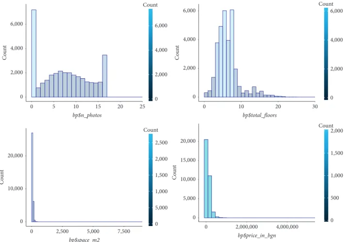
For normally distributed data, approximately 95% of the values lie within 2 standard deviations from the mean. For this reason, observing our data, we can state that only year_end and year_start can be assumed as normally dis-tributed. The standard deviation is not the most suitable measure to study data distribution when the values in a variable are not normally distributed. On the other hand, histograms are one of the most common visual tools to quickly investigate data and make conclusions about central tendency, spread, modality, shape, and outliers. Further-more, histograms support the illustration of the data dis-tribution and serve as a method to envision skewness and kurtosis. Skewness measures the asymmetry, while kurtosis determines “peakedness” compared to the normal distri-bution. These measurements are useful for the
differentiation of extreme values. In positively skewed (right-skewed) data values far from the mode are more regular and usually the mean is greater than the mode. If the skewness is negative, then the mean is less than the mode. Regarding kurtosis, a positive one allows the interpretation that values which are far from the central tendencies are more probable, as well as that the shape is more centrally peaked, but the tail is greater. When the kurtosis is negative, then the peak has wider “shoulders,” compared to the normal distribution [12]. Figure 5 shows the distribution of some of the variables in our dataset.
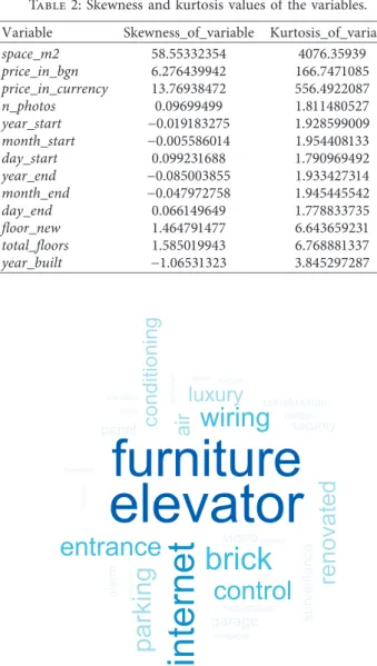
Additionally, Table 2 represents the values of the skewness and the kurtosis of the variables. The negative values imply that the distribution of the data is skewed to the left or negatively. The closer to zero, the slighter the skewness, and likewise if the number is more distant from zero. Oppositely, when the value is greater than zero, the distribution of the variable data is positive/skewed to the left. Concerning the kurtosis, a value smaller than 3 im-plies negative or flat and wide distribution, while a value larger than 3 should be interpreted as high and “slim” distribution [13].
Table 1: Variable list and description.
Variable name Description
lid Listing ID
date_first_seen The date on which the listing of a housing object first appeared online date_last_seen The date on which the listing of a housing object was last seen online rent_or_sell Variable which indicates whether a housing object is for renting or selling
property_type Identifies the type of property being for sale or rent
city The city in which a property is located
neighborhood The neighborhood in which a property is located
street The street on which a property is located
space_m2 The area of a property in m2
price_in_bgn The price of a property in national currency
price_in_currency The price of a property in different currency
currency Specifies the currency
build_type Specifies the building material type
floor Names the floor on which is a property
specials Gives details about the condition of a property
description Text description of a property
n_photos Number of photos which a property has included in the listing
lister_type Specifies whether the listing was made by owner, agent, investor, etc.
lister_username The name of the account from which the listing was made
broker_name The name of the broker (company) which stays behind the listing
1 2 3 4 Maisonette Multiple rooms Room Studio Property_type Agency
(looks like) Bank Builder Investor Owner Agency lister_type 0 50,000 100,000 150,000 df$co un ts
Figure 2: Property types provided by the real estate owner type.
0 1 Property_type 1 2 3 4 Maisonette Multiple rooms Room Studio 0 300 600 900 days_on_market 2.5 5.0 7.5 10.0 12.5 0.0 2.5 5.0 7.5 10.0 12.5 0.0 month_start
4.1.2. Textual Variables. Textual features are extracted from the main description of the house and collected in the variable called specials. They include keywords that describe a property regarding its construction and/or amenities. To give the reader an overview of the features which are
generally used in a listing, a word cloud is created. Figure 6 shows that “elevator” and “furniture” are the most recurrent words in the description of houses, followed by “internet” and “brick.” These features have to be extracted through text modelling as an essential part of the data preparation.
space_m2 price_in_bgn n_photos Year_start Month_start Day_start Year_end Month_end Day_end floor_new total_floors year_built
nbr.val 33740 33398 33408 33740 33740 33740 33740 33740 33740 33740 32517 32517 10586 nbr.null 0 0 0 6104 0 0 0 0 0 0 1356 0 0 nbr.na 0 342 332 0 0 0 0 0 0 0 1223 1223 23154 min 1 39 20 0 2015 1 1 2015 1 1 0 1 1900 max 8065 5280741 3617400 17 2018 12 31 2018 12 31 24 26 2021 range 8064 5280702 3617380 17 3 11 30 3 11 30 24 25 121
sum 2684177 2.71E+09 1.42E+09 265439 68036243 217331 492121 68039886 220340 500516 127731 225508 21146836
median 70 1271 850 8 2017 7 14 2017 7 15 3 6 2006
mean 79.55474 81022.57 42467.9 7.86719 2016.486 6.441346 14.58568 2016.594 6.530528 14.8345 3.92813 6.93508 1997.623 SE.mean 0.584747 657.695 376.769 0.03091 0.005458 0.01761 0.049375 0.005454 0.017644 0.04971 0.015435 0.017281 0.190854 CI.mean.
0.95 1.146124 1289.105 738.4804 0.060584 0.010699 0.034516 0.096777 0.01069 0.034583 0.097434 0.030254 0.033871 0.37411 var 11536.67 1.44E+10 4.74E+09 32.2351 1.005262 10.46293 82.25476 1.003647 10.50374 83.37514 7.747233 9.710418 385.5978 std.dev 107.4089 120194.5 68865.29 5.677596 1.002628 3.234646 9.069441 1.001822 3.240947 9.130999 2.783385 3.116154 19.63664 coef.var 1.350126 1.48347 1.621584 0.72168 0.000497 0.502169 0.621804 0.000497 0.496276 0.615525 0.708578 0.449332 0.00983
price_in_ currency
Figure 4: Numerical variables basic statistics.
0 2,000 4,000 6,000 Count 5 10 15 20 25 0 bp$n_photos 0 1,000 5,000 2,000 1,500 2,500 Count 2,500 5,000 7,500 0 bp$space_m2 0 2,000 4,000 6,000 C oun t 0 2,000 4,000 6,000 Count 10 20 30 0 0 2,000 4,000 6,000 C oun t 0 1,000 500 1,500 2,000 Count 2,000,000 4,000,000 0 bp$price_in_bgn 0 5,000 10,000 15,000 20,000 C oun t 0 10,000 20,000 C oun t
Organized text is usually represented by a table with one token per row. A token is an important component of the text, for instance, a word, which is noteworthy for analysis, and tokenization is the practice of separating the text into tokens. A token can also be a sequence of n words (called n-gram) or even a complete sentence. For instance, in our dataset, several combinations of words such as “entrance control” exist, and they are called bigrams. Also, the variable specials itself contains multiple words which define property features. Thus, it is interesting to examine the relationship and co-occurrence of words. Figure 7 shows the consecutive sequences of words which can be found in the description of a property.
Not only “furniture” and “elevator” are the words that appear most frequently, but also the combination between these two words occurs repeatedly. To examine the corre-lation between words, the so-called phi-coefficient, which is a measure for the binary association of features, was used. This coefficient quantifies the correlation between the probability of two words appearing together and of the same two words appearing independently. Figure 8 illustrates the
four words which appear most often and the words which are most often associated with them. Here, it should be mentioned that, e.g., “under” and “construction” have the same phi-coefficient related to “brick” since “under con-struction” is a predefined special bigram. The same is valid for several more word combinations. Interesting point was to study the correlation between the words “furniture” and “elevator” due to their common occurrence, but the analysis showed a phi-coefficient of only 0.096.
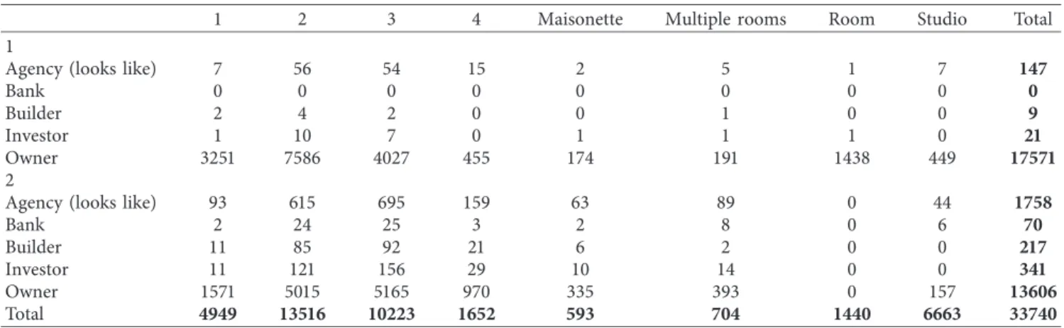
4.1.3. Categorical Variables. The last type of variable that can be found in our dataset is the categorical variable. Table 3 shows that owners are the main listing publishers among the studied ones, and that flats with 2 or 3 rooms have the highest supply level for both rents or sell.
The variable neighborhood contains a large number of possible values. The center region offers slightly more list-ings, but still, none of the neighborhoods preponderates significantly.
Appealing fact, shown in Figure 9, is that the variable type_built usually contains significant values only when a property is listed for selling. When a listing is marked for renting, then the construction type is often unknown. This should be considered during the management of missing values.
4.2. Management of Missing Values. Figure 10 provides an overview of the missing values in the original dataset. The variable space_m2_garden has the greatest amount of missing values since it makes sense only for houses and villas. Nevertheless, for the other types of dwellings, this variable can be informative, and so it was left in the dataset. On the other hand, Homeheed currently concentrates its interest and service to properties which can generically be clustered as “home.” Therefore, the focus of this work is only on properties listed for living purposes, mainly apartments. The type of apartment is stored in the variable property_type, it can assume values such as 1, 2, 3, 4, or multiple rooms, studio, maisonette, and room, and it has no missing values. Our data contain more than 400.000 observations for this type of dwelling. Other types of listings will not be analysed and will be excluded from the dataset.
Other variables with missing values are street, bro-ker_name, and build_type. Given their high percentage of missing values, variables street and broker_name were re-moved from the dataset. Concerning the variable build_type, as it will be discussed later in this document, a decision was taken to split the information contained in this variable, thus creating two new variables: year_built and type_built, containing information relative to the year of building and the building material, respectively. Interestingly, both these variables have a large number of missing values for houses that are for rent, while they present no missing values when houses are for sale. Nevertheless, we decided to remove year_built and type_built from the dataset. In fact, even though both variables contain information for properties that are for sale, the imputation or prediction for 50% of the Table 2: Skewness and kurtosis values of the variables.
Variable Skewness_of_variable Kurtosis_of_variable
space_m2 58.55332354 4076.35939 price_in_bgn 6.276439942 166.7471085 price_in_currency 13.76938472 556.4922087 n_photos 0.09699499 1.811480527 year_start −0.019183275 1.928599009 month_start −0.005586014 1.954408133 day_start 0.099231688 1.790969492 year_end −0.085003855 1.933427314 month_end −0.047972758 1.945445542 day_end 0.066149649 1.778833735 floor_new 1.464791477 6.643659231 total_floors 1.585019943 6.768881337 year_built −1.06531323 3.845297287
Alarm air
0 2000 4000 6000
Alarm wiring Brick elevator Brick parkingBrick under Conditioning internet Conditioning wiring Construction elevatorControl renovated Control securityElevator air Elevator alarm Elevator entrance Elevator furniture Elevator garage Elevator internetElevator luxury Elevator parkingElevator wiring Furniture air Furniture elevator Furniture entranceFurniture garage Furniture luxury Furniture parking Furniture renovated Furniture video Furniture wiringGarage elevator Garage parking Internet entrance Internet furniture Internet renovatedInternet video Luxury air Luxury alarm Luxury wiring Miccs elevator Nofurniture elevatorPanel elevator Parking elevator Parking internet Renovated securitySecurity renovated Surveillance entranceWiring entrance Wiring internet
n
Bi
gr
ams
Figure 7: Relationship between the words in the description.
Correlation Elevator 0.00 0.25 0.50 0.75 1.00 Security Surveillance Video Internet Control Entrance It em 2 Brick 0.00 0.25 0.50 0.75 1.00 Transition Security Leasing Garage Construction Under Correlation It em 2 Internet 0.00 0.25 0.50 0.75 1.00 Renovated Control Entrance Furniture Luxury Wiring Correlation It em 2 Furniture 0.00 0.25 0.50 0.75 1.00 Alarm Internet Luxury Air Conditioning Wiring Correlation It em 2
observation points would be either extremely time con-suming or not be reliable.
Among the other variables with a significant amount of missing values, we also decided to remove the variable lister_username from the dataset.
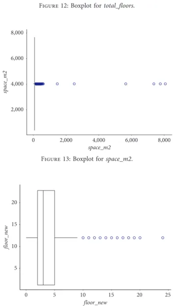
4.3. Management of Outliers. The next step before the transformation of the data is the detection and management of outliers. Outliers may have a significant impact on the data if no actions are taken. For instance, they can increase the error discrepancy and decrease the supremacy of nu-merical tests. Also, outliers can affect normality, as well as the fundamental hypothesis of some statistical models. In practice, an outlier can be interpreted as a value which is 1.5 times the IQR (interquartile range) more extreme than the quartiles of the distribution. The most applicable and useful way to detect an extreme value is by visualizing a boxplot. Figures 11–14 illustrate the boxplots of four features. Ex-treme values that require attention can be seen, as well as long tails in the distribution of the values.
One method which can support a better understanding of these outliers is the breakdown of the variable, which is observed based on the values in another feature. This is called multivariate analysis. Figures 15 and 16 show an example with separating space_m2 based on property_type and by price in currency Bulgarian lev. The scatterplots show Table 3: Cross table for property type by listing provider and by rent or sell.
1 2 3 4 Maisonette Multiple rooms Room Studio Total
1
Agency (looks like) 7 56 54 15 2 5 1 7 147
Bank 0 0 0 0 0 0 0 0 0
Builder 2 4 2 0 0 1 0 0 9
Investor 1 10 7 0 1 1 1 0 21
Owner 3251 7586 4027 455 174 191 1438 449 17571
2
Agency (looks like) 93 615 695 159 63 89 0 44 1758
Bank 2 24 25 3 2 8 0 6 70 Builder 11 85 92 21 6 2 0 0 217 Investor 11 121 156 29 10 14 0 0 341 Owner 1571 5015 5165 970 335 393 0 157 13606 Total 4949 13516 10223 1652 593 704 1440 6663 33740 rent_or_sell 0 1 Beams Brick MICCS Panelt SF NA ty pe_b ui lt 5,000 10,000 15,000 0 Count
Figure 9: type_built by rent or sell.
97.7% 58.8% 53.1% 50.9% 11.7% 9.4% 5.9% 1.1% 1.1% 1.1% Currency price_in_bgn price_in_currency Specials lister_username Floor build_type broker_name Street space_m2_garden 0 30 60 90 Percent missing
Figure 10: Missing values in the studied dataset.
1,000,000 2,000,000 3,000,000 4,000,000 5,000,000 pr ic e_i n_bg n 2,000,000 4,000,000 0 price_in_bgn Figure 11: Boxplot for price_in_bgn.
that there are mainly outliers in 1-, 2-, or 3-room apartments and that places with extreme space have extreme prices.
Extreme points were detected only in two variables, price_in_bgn and space_m2, and their total amount was
small and inconsequential for the overall analysis, so these points were removed from the dataset.
4.4. Data Transformation. In our dataset, different variables have diverse ranges of possible values. Given that some algorithms base their functioning on the distance between observation points to make a prediction, a common scale is needed to assure that none of the features will be dominant. Further, as revealed previously, the distribution of the data in some variables shows skewness, which might represent a difficulty for some of the studied machine learning algo-rithms, and that can be alleviated by scaling the data. Common normalization methods are Min-Max, which scales the range between 0 and 1 and Z-score, which scales values between -1 and 1. In this work, the values have been normalized using Min-Max.
Table 4 reports a set of other modifications that were made to the variables, to obtain a more informative, and potentially more useful, dataset.
Among the other transformations reported in Table 4, it is worth discussing how we decided to transform the textual variable specials. The first task is the removal of punctuation because it has no added value to the information. Fur-thermore, all letters are converted to lower case. This pre-vents multiple extracted copies of the same word. Since the
5 10 15 20 25 0 10 20 total_floors total _f lo or s
Figure 12: Boxplot for total_floors.
0 2,000 4,000 6,000 8,000 space_m2 2,000 4,000 6,000 8,000 sp ac e_m2
Figure 13: Boxplot for space_m2.
5 10 15 20 0 5 10 15 20 25 floor_new floo r_n ew
Figure 14: Boxplot for floor_new.
1 2 3 4 Maisonette Multiple rooms Room Studio 0 2,000 4,000 6,000 8,000 space_m2 pr op er ty_ty pe
Figure 15: Outliers of space_m2 based on property_type.
0 2,000 4,000 6,000 8,000 0 2,000,000 4,000,000 price_in_bgn sp ac e_m2
variable itself contains only keywords, some basic pre-processing procedures, such as stop words removal or stemming (removal of suffices), were not executed. How-ever, the last step was the conversion of a single word into binary variables.
Finally, two new variables were additionally introdu-ced–price_per_m2 and n_features. The first one is calculated based on space_m2 and price_in_bgn. The second one represents the total number of features, including as key-words in the description, available for a listing.
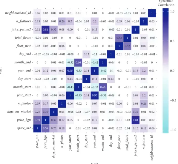
4.5. Feature Selection. The original dataset at our disposal included 19 variables. However, the transformations pre-sented so far have increased the number of variables up to 54, so variable selection techniques have to be applied to choose the most valuable predictors for the model. Filter methods are usually employed as a data preparation step, to select features. First of all, a study of the correlation coef-ficients was performed, to have an idea of the relationship between the continuous variables. Figures 17 and 18 show both the heat matrixes of Pearson and Spearman correlation coefficients.
Both these figures show a significant correlation only between the expected year_start and year_end and between price_bgn and price_per_m2.
Correlation alone can limit the detection of multi-collinearity since it is only pairwise. One of the techniques which support the detection of more complex relationships is the usage of eigenvalues. A small magnitude shows that there is no multicollinearity, while a high range between the values is a signal for significant multicollinearity, which is the case here. The variance inflation factor (VIF), which indicates how much the variance of a regression coefficient is overestimated due to multicollinearity, can be calculated. The minimum possible VIF is equal to 1 and, as a rule of thumb, results between 5 and 10 are considered as indicators for the problem. In our dataset, year_start and year_end showed extreme results above 20 and price_bgn has a result
around 9. To solve this issue, we have decided to remove those variables from the dataset. To examine the significance level between the categorical variables and the target, the Kruskal–Wallis test was performed. A p value which is less than 0.05 indicates a significance level between the groups. Only the variables extracted from the description, telephone_exchange, and elevator had a p value higher than 0.05. All the others, having a smaller p value, cannot be excluded from the dataset.
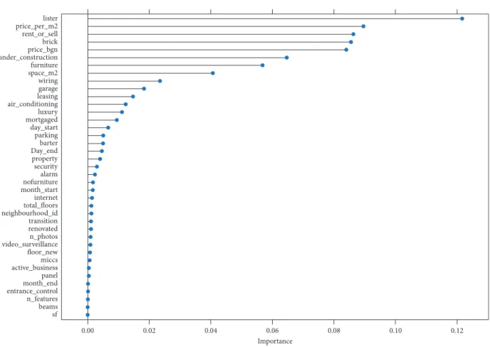
Based on both these filter methods, i.e., correlation and Kruskal–Wallis test, not a significant amount of variables can be excluded. To select the proper variables for the model, we applied an embedded method: Lasso regression. Figure 19 il-lustrates the variables sorted based on their importance and based on the Lasso method.
Observing Figure 19, we can remark that, among the 8 variables that have importance larger than 0.05, two vari-ables are highly correlated between each other: price_per_m2 and price_bgn. Given that these two variables, practically, contain the same type of information, it makes sense to choose only one of them and to remove the other from the dataset. The obvious choice is to keep in the dataset the variable which has the highest importance according to the Lasso algorithm and disregard the other. For this reason, price_per_m2 was kept in the dataset, while price_bgn was removed.
In conclusion, the resulting, final dataset, which was given as an input to the machine learning methods to build the predictive models, contains 7 variables. These variables are (i) lister (ii) rent_or_sell (iii) under_construction (iv) space_m2 (v) brick (vi) furniture (vii) price_per_m2 Table 4: Recoding of original variables.
Variable Original version Recorded version
date_first/
last_seen Both variables are in format “yyyy-mm-dd”
6 new variables were created, namely year_start/end; month start/end; and day_start/end rent_or_sell
property_type “rent” and “sell” 1234 maisonette multiple rooms room studio
Recoded to binary on− 0 rent, 1 for sale recoded completely to numbers-1, 2, 3, 4, 5, 6, 7, 8 lister_type
neighbourhood
Contains many character values with the name of the neighbourhood
An id number was assigned for the different neighbourhoods
lister_type
Contains the levels “owner,” “invester,” “builder,” “blank,” agency (looks like).” The value “agency (looks like)” is a mistake
made during data collection. It represents in reality either investors or builders
Since no strict condition for the recognition between investor and builder was found, the value “agency (looks like)” was randomly replaced to be either builder or investor. New variables with codes from 1
to 4 were created
build_type Originally the variable contains year and building material The variable was split in two new variables-year_built and type_built
specials Text variable in the format [\word1\,”\word2\,”\word3\,”. . .] Binary variables for each word indicating theexistence or lack of this feature floor Originally in the format for example “5 to 10” Split in two new variables floor_new and total_floors
5. Experimental Results
All the results shown in this section have been obtained by performing 30 independent executions of each one of the studied machine learning algorithms. For each one of these executions, a different split of the available data into a learning set and a test set was considered. To obtain this split, 70% of the observations, selected at random with uniform distribution, were considered as the learning set, while the remaining 30% formed the test set. For each one of the studied machine learning methods, the training phase was executed on the learning set and the reported results are the results that have been obtained on the test set. When parameters needed to be set (it is the case, for instance, of the lambda parameter of Lasso, Ridge, and Elastic Net), only the learning set has been used to optimize the parameters’ values, in the following way: the learning set was partitioned into 5 subsets and 5 different training phases were performed with different values of the parameters. In each one of these phases, 4 of these subsets were
used for training, while the other one was used for validation cyclically, so that each one of these 5 subsets was used once and only once for validation (5-fold cross-validation). The set of parameters that were used are the ones who allowed us to obtain the best median results on validation.
Let us begin the discussion of the experimental results by analysing the results obtained by Lasso, Ridge, and Elastic Net. Each of the three models was trained performing a grid search of predefined values of the parameter lambda. The value of lambda which minimizes the RMSE on validation was se-lected. The obtained values of lambda were 0.001 for Lasso, 0.0023 for Ridge, and 0.00014 for Elastic Net. With these values of lambda, the results shown in Table 5 were obtained:
As Table 5 shows, Lasso outperformed both Ridge and Elastic Net both in terms of minimum and median obtained RMSE.
Tables 6 and 7 show, for each one of the used features, the value of the coefficient that was obtained for each one of the studied algorithms. 1 0.59 0.25 0.19 0 0.01 –0.02 0.04 0 –0.02 0.02 –0.04 0.12 0.15 0.06 0.59 1 0.39 0.17 0.05 0 –0.02 0.12 0 –0.05 0.03 0.01 0.84 0.03 0.02 0.25 0.39 1 0.05 –0.08 0.02 –0.07 0.06 0.01 –0.04 –0.03 –0.03 0.32 0.01 0.02 0.19 0.17 0.05 1 0.06 –0.02 0 0.07 –0.01 –0.01 0.06 0 0.08 0.26 0.01 0 0.05 –0.08 0.06 1 –0.43 0.14 0.95 –0.32 –0.08 0 0 0.09 0.2 0.01 0.01 0 0.02 –0.02 –0.43 1 –0.04 –0.33 0.66 0 0 –0.01 0 –0.04 0.01 –0.02 –0.02 –0.07 0 0.14 –0.04 1 0.14 –0.01 0.13 0 0 –0.01 0.03 0 0.04 0.12 0.06 0.07 0.95 –0.33 0.14 1 –0.42 –0.1 –0.01 –0.01 0.15 0.2 0.01 0 0 0.01 –0.01 –0.32 0.66 –0.01 –0.42 1 –0.04 0 0 0 –0.03 0 –0.02 –0.05 –0.04 –0.01 –0.08 0 0.13 –0.1 –0.04 1 0.01 0.01 –0.05 -0.01 -0.01 0.02 0.03 –0.03 0.06 0 0 0 –0.01 0 0.01 1 0.52 0.01 0.09 -0.03 –0.04 0.01 –0.03 0 0 –0.01 0 –0.01 0 0.01 0.52 1 0.01 0.06 -0.05 0.12 0.84 0.32 0.08 0.09 0 –0.01 0.15 0 –0.05 0.01 0.01 1 –0.03 0.01 0.15 0.03 0.01 0.26 0.2 –0.04 0.03 0.2 –0.03 –0.01 0.09 0.06 –0.03 1 0.03 0.06 0.02 0.02 0.01 0.01 0.01 0 0.01 0 –0.01 –0.03 –0.05 0.01 0.03 1 –1.0 –0.5 0.0 0.5 1.0 Spearman correlation space_m2 price_bgn days_on_market n_photos year_start month_start day_start year_end month_end day_end floor_new total_floors price_per_m2 n_features neighbourhood_id Var 1 ne ig hb ou rhood _id da ys_o n_m ar ke t pr ic e_per_m2 mon th _sta rt m on th_en d total _f lo or s n_f ea tu re s ye ar _sta rt fl oo r_ ne w da y_ sta rt sp ac e_m2 n_p ho to s pr ic e_bg n ye ar_en d da y_en d Var2
Tables 6 and 7 give an idea of the relative importance of the variables for each one of the studied algorithms. As we can see, none of the coefficients was equal to zero, except for the coefficient of variable price_per_m2 for Lasso and Elastic Net. This confirms the appropriateness of the work that was done in the feature selection phase, corroborating that the 7 selected features are important for the prediction.
Let us now discuss the results obtained by Artificial Neural Networks. A grid search was performed to look for appropriate values of the number of hidden layers and the number of units per hidden layer. The results that returned the best median results on validation were 2 hidden layers, 3 units in the first hidden layer, and 2 units in the second hidden layer. Figure 20 illustrates the trained Neural Net-work that was possible to obtain with this configuration. The black lines give visibility on the connections and their weights, while the blue lines and values represent the bias term added on each step.
Figure 21 reports a comparison between the Neural Network and the Lasso regression, showing real vs predicted values. The closer the data points to the line, the better the model (theoretically, in the best-case scenario, the data
points should align perfectly with the line, when the RMSE is equal to 0).
The scatterplots show that the Neural Network has slightly more distant data points from the line than the Lasso. This gives a visual indication that Lasso may be a more accurate algorithm than Neural Networks for the studied problem. This qualitative result is also corroborated quan-titatively: the RMSE obtained by the Neural Network is equal to 0.065, which means that Lasso performs slightly better.
Besides that one may also consider that Neural Networks are in general more complicated for interpretation and explanation.
Finally, to strengthen the robustness of the results ob-tained using Lasso, we perform a comparison against other well-known machine learning techniques commonly employed to address regression problems, namely, random forests (RFs), support vector regression (SVR), and k-nearest neighbors (K-NN). The reader is referred to the material in Appendix A for a brief overview of these techniques. To ensure a fair comparison, the values of the parameters characterizing the different techniques were chosen by performing a preliminary tuning phase. In particular, similar
1 0.59 0.25 0.19 0 0.01 –0.02 0.04 0 –0.02 0.02 –0.04 0.12 0.15 0.06 0.59 1 0.39 0.17 0.05 0 –0.02 0.12 0 –0.05 0.03 0.01 0.84 0.03 0.02 0.25 0.39 1 0.05 –0.08 0.02 –0.07 0.06 0.01 –0.04 -0.03 –0.03 0.32 0.01 0.02 0.19 0.17 0.05 1 0.06 –0.02 0 0.07 -0.01 –0.01 0.06 0 0.08 0.26 0.01 0 0.05 –0.08 0.06 1 –0.43 0.14 0.95 –0.32 –0.08 0 0 0.09 0.2 0.01 0.01 0 0.02 –0.02 –0.43 1 –0.04 –0.33 0.66 0 0 –0.01 0 –0.04 0.01 –0.02 –0.02 –0.07 0 0.14 –0.04 1 0.14 –0.01 0.13 0 0 –0.01 0.03 0 0.04 0.12 0.06 0.07 0.95 –0.33 0.14 1 –0.42 –0.1 –0.01 –0.01 0.15 0.2 0.01 0 0 0.01 –0.01 –0.32 0.66 –0.01 –0.42 1 –0.04 0 0 0 –0.03 0 –0.02 –0.05 –0.04 –0.01 –0.08 0 0.13 –0.1 –0.04 1 0.01 0.01 –0.05 –0.01 –0.01 0.02 0.03 –0.03 0.06 0 0 0 –0.01 0 0.01 1 0.52 0.01 0.09 –0.03 0.04 0.01 –0.03 0 0 –0.01 0 –0.01 0 0.01 0.52 1 0.01 0.06 –0.05 0.12 0.84 0.32 0.08 0.09 0 –0.01 0.15 0 –0.05 0.01 0.01 1 –0.03 0.01 0.15 0.03 0.01 0.26 0.2 –0.04 0.03 0.2 –0.03 –0.01 0.09 0.06 –0.03 1 0.03 0.06 0.02 0.02 0.01 0.01 0.01 0 0.01 0 –0.01 –0.03 –0.05 0.01 0.03 1 –1.0 –0.5 0.0 0.5 1.0 Spearman Correlation space_m2 price_bgn days_on_market n_photos year_start month_start day_start year_end month_end day_end floor_new total_floors price_per_m2 n_features neighbourhood_id Var 1 neighbourhood_id days_on_market price+_per_m2 month_start month_end
year_satart floor_new total_floors n_features
price_bgn
space_m2 n_photos day_start year_end day_end
Var2
to the experiments performed with Neural Networks and Lasso, we performed a grid search to determine the most suitable parameters for the considered machine learning techniques.
Focusing on RFs, the tuning phase returned a value of 70 for the maxnodes parameter (i.e., the parameter that limits the total number of nodes in each tree), 1000 for the number of trees in the random forest, and the function used to
measure the quality of a split in the trees was the Gini impurity. The RF with this configuration returned a median RMSE equal to 0.073.
Focusing on K-NN, it is important to highlight the importance of the parameter k (i.e., number of neighbors) on the performance of the model. In particular, the literature reports that a model with a very low value of k may tend to overfit the data, while higher k values can lead to under-fitting. The grid search procedure returned a value of k equal to 15, leading to a final model with an RMSE of 0.064. Though this value is comparable to the one achieved with Lasso, K-NN has some weaknesses in the context of the problem studied here. In particular, K-NN requires an unbearable amount of time to return a prediction for unseen data since it has to compute the distance between each new
Importance sf beams n_features entrance_control month_end panel active_business miccs floor_new video_surveillance n_photos renovated transition neighbourhood_id total_floors internet month_start nofurniture alarm security property Day_end barter parking day_start mortgaged luxury air_conditioning leasinggarage wiring space_m2 furniture under_construction price_bgn brick rent_or_sell price_per_m2 lister 0.00 0.02 0.04 0.06 0.08 0.10 0.12
Figure 19: Lasso variables importance.
Table 5: RMSE obtained by Lasso, Ridge, and Elastic Net. Model Min 1st Qu. Median Mean 3rd Qu. Max NAs Ridge 0.059 0.065 0.068 0.067 0.070 0.073 0 Lasso 0.056 0.064 0.066 0.067 0.070 0.081 0 Elastic 0.059 0.065 0.068 0.067 0.070 0.073 0
Table 6: Ridge regression coefficients.
Variable Coef. (Intercept) 0.007812742613 rent_or_sell 0.017990042310 space_m2 0.087954307932 brick 0.006890894870 furniture −0.005648094327 under_construction 0.023199993261 price_per_m2 0.012193552241 lister 0.126633821677
Table 7: Coefficients of Lasso and Elastic Net.
Variable Coef. Lasso Coef. Elastic
(Intercept) 0.008262840044 0.006914658626 rent_or_sell 0.020773920773 0.021302049363 space_m2 0.081148777731 0.088121228126 brick 0.006277781636 0.006389871295 furniture −0.004166719412 −0.004836976890 under_construction 0.020923002635 0.022619172277 price_per_m2 0 0 lister 0.127546013431 0.130465654935
–1.21835 6.13114 0.91511 lister –0.70376 –0.11556 –0.05591 price_per_m2 –0.94717 –0.47041 0.4162 under_construction –0.05687 0.21111 –0.34204 furniture 0.35840.20533 0.11747 brick 1.72687–1.41347 4.06222 space_m2 –0.26295 0.26135 0.06656 rent_or_sell –0.49505 0.66393 –0.3 0478 –1.85063 2.77573 –1.42974 0.44641 –1.00307 days_on_market 0.06949 0.79916 –1 .96525 1 2.12953 –0.613 59 1 –0. 231 4 1
Figure 20: The best Neural Network that we were able to obtain in our experiments.
0 200 400 600 800 1000 50 100 150 test$days_on_market p redic t.nn$net.r esul t NN (a) 0.0 0.2 0.4 0.6 0.8 1.0 0.00 0.05 0.10 0.15 0.20 test_$days_on_market pr ed_las so2 Lasso (b) Figure 21: Continued.
observation and the samples in the training set. Moreover, the interpretability of a model generated by means of a penalized regression is higher than the one of K-NN, since features’ importance cannot be extracted from K-NN.
The performance of the last machine learning technique considered, SVR, generally depends on the choice of the kernel function. The kernel function defines the relation-ship/distance between the support vector and the target, by transforming the nonlinear input space into a linear space. The basic concept behind SVR is that the maximum ad-missible error for the prediction should be below a certain value defined as epsilon. To avoid overfitting, the regression is penalized by the usage of a cost parameter. In the ex-perimental phase, we used the automated kernel function selection, but to define penalty cost and epsilon (maximum allowed error), we performed a grid search. Performing the experiments with epsilon � 0.5 and the cost parameter equal to 4.57, we obtained a median RMSE of 0.066.
Table 8 presents several performance measures to summarize and compare the models trained for the pre-sented problem. MAE (mean absolute error) and MDAE (median absolute error) are both suitable measures as the data taken into account are characterized by some extreme values for DOM. The explained variance score takes into consideration the mean error, while R2does not consider the mean error in the calculation and this makes the metric a bit more biased, which may lead to over- or underestimating the model in terms of how well the predictors explain the target. All in all, it is possible to state that despite its simplicity, Lasso is the technique that we found most appropriate to address the problem at hand. In particular, it produced a competitive performance (i.e., low error) by also allowing us to analyse the most important features that characterize the problem. Section 5.1 is dedicated to this analysis.
5.1. Feature Importance in the Model Found by Lasso. One of the most known methods to measure the importance of features in a learned predictive model consists of mea-suring the increase in the error of the model, after modifying the values of the features, for instance, shuffling their values
along with the different observations. In other words, a given feature is considered less or not important if rearranging its values does not lead to any change in the model’s error, and it is considered as important if it leads to a significant modification of the error. One of the interesting points of this method is that it takes into account not only the re-lationship of a feature with the output variable, but also with all the rest of the features. Additionally, the permutation importance does not require retraining of the model, but just a simple shuffling of the values of the features [14].
Figure 22 shows the features, sorted according to their importance (from the most important one that is reported at the top to the less important one that is reported at the bottom). For each feature, its importance is measured as a difference in the RMSE between the model executed with the original values of the feature and the model executed after shuffling. Table 9 gives detailed information on the results of the features importance test.
These results show that lister is considered as the most important feature by the Lasso model, followed, in the order by rent_or_sell, under_construction, space_m2, brick, and furniture. Finally, price_per_m2 was considered as the less predictive feature.
6. Conclusions and Future Work
The objective of this paper was to develop a model to predict the days_on_market variable by applying several algorithms, in particular, Lasso, Ridge, and Elastic Net regressions and Neural Networks. The starting point of the work was the formulation of the following research questions, which will be answered in the upcoming paragraphs:
(1) Can a machine learning algorithm predict the days_on_market variable for the housing units? (2) Which features effectively influence the property
attractiveness for the customer target?
The various features were investigated and transformed to identify the key factors that affect the attractiveness of a property, which resulted in the reduction of features used in
0.0 0.2 0.4 0.6 0.8 1.0 0.05 0.10 0.15 test_$days_on_market pr ed ict_n n$n et.r es ul t NN Lasso (c)
the model to 7. Then, the studied algorithms were trained and Lasso regression outperformed the other studied al-gorithms. In conclusion, we were able to develop an accurate predictive model using Lasso regression, to predict the in-dependent variable days_on_market with a selection of discriminators, which will be discussed in the second re-search question. The answer to the second question (2) was closely related to the findings of the first one: recognizing the features which make a property more interesting to the market. As many studies focus on measuring the effect of factors on houses’ price, here the point of interest was measuring the effect of features on attractiveness. Based on this particular dataset, the features which have the most influence on the days_on_market are lister, rent_or_sell, under_construction, space_m2, brick, and furniture. One of the main limitations of this work is given by the available data. For instance, a significant amount of the variable characters was in Cyrillic, and while it was possible to translate some of them in English, others contained a major number of characters which made the automatic and correct
translation impossible. For example, analysing further the full description of the listings, or considering the names of the agencies/owners who published the listings could pro-vide deeper insights.
To improve this work, several supplementary steps can be taken in the future. In the data collection phase, which was not part of the scope of this paper, additional data sources can be taken into account. For example, data for the neighborhood and residential profile (schools, su-permarkets, transport, etc) can be collected and included in the research. The same is valid for other factors that influence the market. Additionally, as mentioned previ-ously, the real days on market for a property were not available and known in this dataset. To assure the reability of the outcome, information about properties’ li-quidity needs to be collected. This is not only time consuming but also a long-term task since such infor-mation would be available only if it provided directly by agencies and owners. Furthermore, the data used here were only for one city; a more complex dataset covering Table 8: Model comparison—performance measures.
Model RMSE MAE MDAE R2 Explained variance score
Random forest 0. 073 0.0399 0. 0202 0. 3625 17.5037 Elastic Net 0.065 0.0341 0. 0176 0.1983 9.5736 Lasso 0.064 0.0340 0.0177 0.1832 8.8431 Ridge 0.065 0.0341 0. 0176 0.1942 9.3746 ANN 0.065 0.0339 0.0160 0.2 9.6594 K-NN 0.064 0.0331 0.0155 0.2394 11.5575 SVR 0.066 0.0396 0.0321 0.0761 3.6757 price_per_m2 furniture brick space_m2 under_construction rent_or_sell lister 0.96 1.00 1.04 1.08 1.12
Feature importance (loss: rmse)
Fe
at
ur
e
Figure 22: Feature importance in the model.
Table 9: Feature importance in the model.
Variable Importance.05 Importance Importance.95 Permutation error
lister 1.0611371 1.0676099 1.119868 0.07243278 rent_or_sell 0.9945100 1.0278727 1.072171 0.06973678 under_construction 0.9973978 1.0262011 1.030145 0.06962337 space_m2 0.9818909 1.0215203 1.032234 0.06930579 brick 0.9752772 1.0109712 1.038632 0.06859008 furniture 0.9664737 1.0071756 1.037656 0.06833257 price_per_m2 0.9698690 0.9905373 1.030250 0.06720373
various cities and regions with their own specifications would be more informative. In the long term, we plan to collect demographics, users profile, and in-app behavior data. Such information together with macroeconomic statistics for purchasing power, banking interest rates, employment level, wage rates, etc., can provide a broader picture not only about the market, but also about the factors which influence home preferences and attrac-tiveness. Not to forget news and media data, which both can reveal interesting patterns for customer behavior and market fluctuations, as well as can provide some insights for the reputation of different agencies. Last but not least, another field of potential research involves the use of other machine learning algorithms, such as a k-nearest neigh-bor, support vector machines, and random forest.
Appendix
Regression analysis is a statistical technique that models and approximates the relationship between a dependent variable and one or more independent variables. In the case of this study, the dependent variable is days_on_market (DOM), while the independent variables resulted from a complex phase of data preprocessing, described in Section 4. This Appendix describes the different techniques used in the paper to address the regression problem at hand.
A.1. Lasso, Ridge, and Elastic Net. Simple linear regression, also known as ordinary least squares (OLS) attempts to minimize the sum of error squared. The error, in this case, is the difference between the actual (observed) data point and its predicted value. The equation for this model is referred to as the cost function and is a way to find the optimal error by minimizing and measuring it:
M i�1 yi− ^yi2� M i�1 yi− p j�0 wj× wij ⎛ ⎝ ⎞⎠ 2 . (A.1)
The gradient descent algorithm is used to find the op-timal cost function by going over several iterations. But the data we need to define and analyse are not always so easy to characterize with the base OLS model. One situation is the data showing multicollinearity, this is when predictor var-iables are correlated to each other and the response variable. To produce a more accurate model of complex data, we can add a penalty term to the OLS equation. A penalty adds a bias towards certain values. These are known as L1 regu-larization (or Lasso regression) and L2 reguregu-larization (or Ridge regression).
Ridge regression adds the following penalty term, called L2 term, to the OLS equation:
+λ p
j�0
w2j. (A.2)
The L2 term is equal to the square of the magnitude of the coefficients. In this case, if lambda (λ) is zero, then the
equation is the basic OLS. If lambda is greater than zero, then a constraint is added to the coefficients. This constraint has the objective of minimizing the coefficients (or, informally speaking, shrinking). The values of the coefficients tend towards zero as the values of lambda get larger. Shrinking the coefficients leads to lower variance and in turn a lower error value. Therefore Ridge regression decreases the complexity of a model. However, Ridge does not reduce the number of variables it rather just shrinks their effect.
Lasso (least absolute shrinkage and selection operator) regression uses the L1 penalty term, which is equal to the absolute value of the magnitude of the coefficients:
+λ p j�0 wj . (A.3)
Analogously to Ridge regression, also for Lasso, a lambda value equal to zero corresponds to the basic OLS equation. However, given an appropriate lambda value, Lasso can drive some coefficients to zero. The larger the value of lambda, the more features are shrunk to zero. This can eliminate some features and give us a subset of predictors that helps mitigate multicollinearity and model complexity. If a variable is not shrunk to zero, it means that the variable is important. In other words, L1 regularization allows for feature selection (sparse selection).
A third commonly used model of regression is the Elastic Net, which incorporates penalties from both L1 and L2 regularization: ni�1yi− xji^β2 2n +λ 1 − α 2 m j�1 ^ β2j +α m j�1 ^ βj ⎛ ⎝ ⎞⎠. (A.4)
In addition to choosing a value for the lambda pa-rameter, Elastic Net also allows us to tune the alpha (α) parameter. A value of alpha equal to zero corresponds to Ridge; a value of alpha equal to one corresponds to Lasso. If we choose an alpha value between 0 and 1, we can incor-porate penalties from both L1 and L2 regularization and alpha allows us to decide the relative importance of these two penalties. The interested reader is referred to Fonti [15] for deepening the functioning and properties of the Lasso, Ridge, and Elastic Net regression methods.
A.2. Artificial Neural Networks. An Artificial Neural Net-work (ANN) is a computational model based on the structure and functions of biological neural networks. It is composed of a set of elementary computational units, called neurons, strongly interconnected between each other by means of connections, or synapses, characterized by a weight. An ANN encodes a function (or model) that can produce outputs once inputs are presented to it. Supervised learning ANNs that are the ones studied in this paper have the objective of returning the expected outputs for each one of the input vectors contained in a given dataset. The learning phase, aimed at obtaining this expected input/ output match, consists in a modification of the weights of the
connections in the network. Every single neuron can be represented as shown in Figure 23.
Once the values of the set of weights of the connections entering into a neuron have been established, the output of the neuron is calculated by
y � f n i�1 wixi+θ ⎛ ⎝ ⎞⎠. (A.5)
In an ANN, neurons are usually organized into layers. Supervised learning ANNs are formed by three different types of layers of artificial neurons:
(i) Input layer (ii) Hidden layer (iii) Output layer
The input layer communicates with the external environ-ment that presents data to the neural network. Its job is to deal with all the input values. These input values are transferred to the hidden layers, which are explained below. Every input neuron represents some independent variable that has an in-fluence over the output of the neural network. The hidden layers are intermediate layers, found between the input layer and the output layer. The job of each hidden layer is to process the inputs obtained by its previous layer. Finally, the output layer contains the units that return the computed result to the outside world. The general structure of a feed-forward ANN, i.e., one of the most diffused types of supervised ANN and the one used in this work, is shown in Figure 24.
Several learning rules exist, aimed at looking for a configuration of the connection weights that allow a perfect input/output match. One of the most diffused ones and the one used in this paper is called backpropagation. The in-terested reader is referred to Gurney [16] to deepen the subject.
A.3. Support Vector Regression. Support vector machines (SVM) were introduced in [17], for classification problems. The objective is looking for the optimal separating hyper-plane between classes. The points lying on classes’ bound-aries are called support vectors, and the in-between space, the hyperplane; when a linear separator is not able to find a solution, data points are projected into a higher-dimensional space, where the before nonlinearly separable points become linearly separable, using kernel functions. The whole task can be formulated as a quadratic optimization problem that can be solved with exact techniques. In Figure 25, an example of a linearly separable classification problem solved using SVM is presented. SVM aims at maximizing the margin between the support vectors and the hyperplane.
One year after the introduction of SVM, Smola [18] presented an alternative loss function, which allowed SVM to also be applied to regression problems. In SVR, the idea is to map the data events X into a k-dimensional feature space
F, through a nonlinear mapping φj(X), so that it is possible
to fit a linear regression model to the data points in this space. The obtained linear learner is then used to forecast in
the new feature space. Once again, the mapping from the input space into the new feature space is defined by the kernel function. One of the most attractive characteristics of SVR is related with the model errors; instead of minimizing the observed training error, SVR minimizes a combination of the training error and a regularization term, aimed at improving the generalization ability of the model. Other attractive properties of SVR are related to the use of kernel functions, which make them applicable both to linear and nonlinear forecasting problems, and the absence of local minima in the error surface due to the convexity of the fitness function and its constraints. Given
(i) Training dataset T, represented by
T � x 1, y1, x2, y2, . . . , xm, ym, (A.6)
where x ∈ X ⊂ Rn are the training inputs and y∈ Y ⊂ R are the training expected outputs;
. . . x1 x2 xn w1 w2 wn +1 y Input values Weights Threshold Output value θ
Figure 23: General structure of an artificial neuron.
x1 x2 xn ym y1 y2 . . . . . . . . . . . . . . . . . . . . .
Hidden neurons Output neurons
Figure 24: Architecture of a feed-forward ANN.
Support vectors
Separating hyperplane
Margin
![Figure 1: Loans interest rates Bulgaria [1] and amount of home loans [1].](https://thumb-eu.123doks.com/thumbv2/123dok_br/15570430.1047952/2.900.105.801.113.313/figure-loans-rates-bulgaria-home-loans.webp)