A Work Project, presented as part of the requirements for the Award of a Master Degree in Finance from the NOVA – School of Business and Economics.
USING THE BAIDU INDEX TO PREDICT CHINESE
HOUSING PRICE AND VOLUME
-- A SURVEY-BASED KEYWORD SELECTION APPROACH
ZHANG QUANXING STUDENT NUMBER: 25507
A Project carried out on the Master in Finance Program, under the supervision of: Mike Langen (Maastricht University)
Professor Sofia F. Franco (NOVA – School of Business and Economics)
Using the Baidu Index to Predict Chinese Housing Price and
Volume -- A Survey-based Keyword Selection Approach
ABSTRACT
The paper uses a survey-based keyword selection approach to examine the effect of the Baidu Index on Chinese real estate trends. After obtaining weights from 546 questionnaires to composite the indexes, I find that in the transaction volume model with the survey-based indexes, the adjusted R2 increases by 8.240 percentage points compared to the baseline model. Such improvement also exists in a forecasting test, reducing the Mean Absolute Error by 2.931 percent and the Mean Squared Error by 5.079 percent. The paper further contributes to the keyword selection method and the model by exploiting an up-to-date dataset.
1. Introduction
Including search engine data as one of the data sources is nowadays becoming more popular in academia. For researchers in real estate, it has the potential to help predict housing price and transaction volume. After Wu and Brynjolfsson (2015)’s application of the Google Trend to study its predictive power to housing price and transaction volume as a proxy of public attention on real estate, the academia use search engine data when studying this area. Studies on Chinese real estate trends also apply search engine data, and they prefer using the source from the Baidu Index to enjoy benefits from a more extensive local user base. The Baidu Index is similar to the Google Trend but more focused on its Chinese language users. It is available to thepublic by providing information on users’ interest and characteristics based on one of the biggest databases on the Internet collected from searching behaviours. This paper continues using the same source to study housing price and transaction volume trends for the Chinese real estate market by focusing on particular urban markets.
The first motivation of this study is to investigate if using people’s keyword preferences by directly asking them can help develop a new keyword selection method. The Baidu Index series are reflections of keywords activeness of searches, and researchers have to link these keywords to real estate data. Choosing, grouping and weighing the Baidu Index series differently from various related keywords can change results. Previous studies in Chinese academia choose the keywords in real estate generally based on author’s selection (Hong and Li, 2015) or correlations (Cao and Mu, 2016), but such keyword selection processes may not reflect the actual behaviour of search engine users.
Although the keyword selection process helps sort the data from search engines, the goal for researchers is to explore some practical implications by constructing their prediction models. As such another goal of this work is to include some factors such as a certain level of interdependence to improve the model. Moreover, in the Chinese context, the last motivation attributes to some new data after the latest housing boom starting from 2015 in major Chinese cities. These new data enrich the available dataset for studies of its relations with the Baidu Index, but the predictive power of the Baidu Index to real estate trends needs to be revisited.
This paper investigates the effect of composite Baidu Indexes combined with keywords based on a survey on providing explanatory power to housing price and volume trend in the Chinese real estate market. I decompose the analysis into three parts: create a more behaviour-based proxy from a range of individual Baidu Index keywords, build a prediction model with the proxy and compare the forecast errors with a baseline without Baidu Index. First, I obtain the weekly Baidu Index series of 25 keywords according to the results of a survey and composite them into three categories. After solving the stationarity problem of the time series,
I propose a model with the weekly secondary market average price data and transaction volumes of commercial apartments in four representative cities in China (Beijing, Shanghai, Guangzhou, and Chengdu) to examine whether the survey-based composite indexes add predictive power. Then I calculate the forecast errors of each model for a prediction test of the first six months of 2018 to compare their forecasting performance.
Based on 546 surveys collected, the outperforming category is the keywords from the financing category. Participants in the survey assign weights of individual keywords on average ranging between 17% and 24%. Using 3 different ways of keyword compositions and the index data covering the period from 2011-2017, I find that the model with the survey-based indexes increases the adjusted R2 for both models of housing price and housing transaction volume. For the model of housing transaction volume, adding the survey-based composite indexes increases the adjusted R2 by 8.240 percentage points, decreases the Mean Absolute Error by 2.931 percent and lowers the Mean Squared Error by 5.079 percent, compared with the respective values in the baseline model. Overall, the survey-based indexes have better performance compared to the equally-weighted indexes and the search-volume-based indexes.
The paper contributes to the literature in several ways. Previous studies like Kulkarni et al. (2009), Yang et al. (2013) and Pu et al. (2018) have focused on the predictive power of search engine data on real estate. However, the selection of different sets of keywords has a significant impact on the empirical results. More attention is needed when selecting the index data from a variety of keywords. This study develops a new keyword selection method to acquire trends with behavioural supports of public attention to real estate, and thus it further fills the gap in the keyword selection process.
In addition, this study is the first study to my knowledge that uses survey results to generate composite trends from search engine data. Previous studies such as Cao and Mu (2016) and Yang et al. (2013) either plug in individual keywords into the model or use correlation coefficients to composite. The correlation-based method has statistical advantages to link the indexes to real estate price or transaction volume trend. However, such a method does not have sufficient support from the behavioural side because the process of choosing the keywords to search relies on searcher’s subjective decision. Through this study, one can learn from the behavioural choice of keywords from survey samples.
The limited number of observations available from Baidu leads to a constrained number of variables for estimation, so another relevant contribution of this study is that it groups the keywords into different categories. It can separate the impact from different perspectives and exploit the interdependence of time series to find a predictive model for real estate prediction based on a higher time-frequency search engine data. Compared to previous studies from Dong
et al. (2014) or Pu et al. (2018) who include individual indexes, grouping into categories would lower the number of coefficients to estimate. It helps construct a better model when the time series observations are limited as the Baidu Index just starts from 2011. Finally, it is the first time that a study of this kind takes account of the interdependency when modelling.
The remainder of the paper is organized as follows. Section 2 provides a brief literature review and discusses existing empirical results to develop testable hypotheses. A detailed design regarding the survey and the model is followed in section 3. Then section 4 documents the empirical results from this study and offers a discussion. Finally, section 5 reviews the main implications, discusses the limitations and suggests a few directions for future studies.
2. Literature Review
2.1 Existing studies
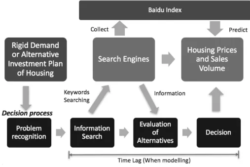
Before the Internet has gone into people’s life, research on the relationship between consumer’s information demand and housing prices was mainly based on expectations. Case and Shiller (1988) find that people have higher expectations about the increase in housing prices in Los Angeles, where housing prices have been increasing rapidly, by conducting a survey with 886 responses from a mailing list of persons who bought homes in May 1988. These authors conduct the survey approach again in 2003 and conclude that the extreme self-confidence of consumers is the main reason for the rise in housing prices during the studied period. People typically collect all the information they can get before taking their decisions. For participants in real estate markets, they also go through such a decision-making process. Shang and Qiu (2008) conclude that the real estate is a kind of special good and the consumers are very likely to be highly involved, that is, spending a lot of time and effort searching for information. Since search engines have become an important source of information flow, searching the most relevant keywords based on their perceptions of the real estate market is very common for Internet users before they decide. Dong et al. (2014) conclude that search engines can lower consumers’ costs of collecting the housing information. The framework from search engines data to housing prices and sales volume is shown in Figure 1, elaborating how search engines are involved in the buyer’s decision process. Real estate buyers typically go through an information searching stage before making their decisions. When they turn to search engines for information, Baidu records search volumes of the keywords they input and shows them in the Baidu Index. Knowing that real estate purchasing decisions have a direct effect on housing prices and sales volume, therefore, as the reflection of the information searching stage for their final decisions, the Baidu Index data can offer insights on the housing price and sales
volume. The time lag between the information searching stage and the final decision also suggests that information from the Baidu Index is a leading indicator of these real estate series.
Figure 1: Logical Framework Diagram for Search Engines Data to Housing Prices and Sales Volume
Therefore, researchers in real estate start recognising the value of using search engines data and other web search data. Kulkarni et al. (2009) test the relationship between online keyword searches and the housing price index for 20 cities in the United States, where they verify a relationship via the Granger Causality between the keywords and the housing price index. The change of certain keywords’ search volume also reflects changes in demand. Pan et al. (2012) establish the link of search engine data to the demand for hotel rooms and it provides additional explanatory power to the prediction model. They find that the searched keyword trends are early indicators of consumer’s interest and are applicable in predictions of activities like hotel occupancy, expenditure and the attendance of events. Wu and Brynjolfsson (2015) conclude that consumers can improve their decision process using the information in search engines. They include the Google Trend’s data into the prediction model in the US housing market, discovering that the housing search index is highly correlated with the home sales. From the perspective of the whole country, the average forecast error after including search data is lower, compared to the prediction model based on traditional indicators. Besides the Google Trend, Park et al. (2015) apply machine learning algorithms to study the price of Fairfax Country, in order to overcome the limitations of assumptions and estimations of conventional statistical approaches but the study only focuses on a specific region while the location is one of the most important factors in real estate studies.
When the methodology of including search engine series in real estate research started to be used in the Chinese context, researchers also applied the Google Trend’s data (e.g. Yang et.al., 2013 and Wu et al., 2015). However, choosing the most representative data source in the China-based studies become relevant for researchers in real estate, especially after Google’s exit of its search engine service in mainland China after 2010. Due to the advantages of a bigger user base in Chinese local search engines like Baidu proposed by Vaughan and Chen (2015), more and more studies of this kind favour the data from the Baidu Index, such as Dong et al. (2014), Hong and Li (2015) and Cao and Mou (2016).
Though a set of literature has documented the predictive power of search engine data on real estate, these studies aim to establish the link between search engine data and housing market trend, where their keywords are determined by experience from experts or recommendations from the search engine (e.g. Cao and Mu, 2016 and Yang et al., 2013). To narrow the range of keywords, these studies rank the keywords based on their correlations with the dependent variables. After having the range of the keywords, individual indexes can be retrieved from the search engine database when entering a single keyword, like an index with the keyword “Housing Price” or an index with the keyword “Housing Price Trend”. These individual ones are the typical case for the index data. In previous literature, Dong et al. (2014) use the selected individual indexes directly in the model. Pu et al. (2018) also plug the individual indexes in the model when studying the short-term trend of Wuhan’s housing price.
Other sets of studies choose to group these individual indexes to a composite one before they go to the actual analysis. Although using the most common keyword is the simplest way to reflect a certain category of information, having users who search a few keywords in the same category is even more common. A better reflection of behaviours in search engine trends needs to combine the patterns in some way, namely, like building an index in the stock market, construct a composite index for a category using individual indexes. For example, indexes of “Housing Price” and “Housing price Trend” are two individual indexes but one can combine them into a single composite index called “Housing Price” (pricing status). Previously, Bai et al. (2015) group the individual indexes into three main categories: “Economic Environment”, “Government Policy” and “Real Estate General” before they are included into the prediction model. Cao and Mu (2016) find that consumers put less attention to the affordable housing plan of the government and the least attention to land status. They also document that consumers focus most on the pricing information, stating that the strongest sensitivity of Chinese consumers on housing price. Besides the pricing status, consumers are aware of financing, administrative, fiscal, policy control issues, and other general information. These studies reveal the importance of grouping keywords in different categories.
Previous literature mainly constructs composite indexes using the correlation-weighed method. The construction of correlation-weighed indexes has a two-stage process. Researchers like Bai et al. (2015), Cao and Mu (2016) select in the first stage a range of keywords based on experience from experts in real estate then run each of the individual indexes with the dependent variables to find their Pearson correlation coefficients. The correlation coefficients usually have positive values as the interest of these studies is to find which keywords are representative of the corresponding category. By eliminating those without having significant correlations, they obtain a keyword set for each category. In the second stage, they determine the weight of each keyword according to its ranking of the correlation coefficient in the same category before they are plugged into the model.
In terms of modelling, past studies preliminarily construct the prediction model to test the predictability, but their model selections vary. And many of them have constraints caused by the limited number of observations from the data. Jiang et al. (2016) apply the Auto-Regressive and Moving Average (ARMA) model. Their research on Shanghai’s new apartments’ price reveals a positive relationship of the price trend, meaning that the housing price booms together with the search volume and adding the Baidu Index in the model increase the accuracy of 20.8 percent. Pu et al. (2018) further compare another 6 different models in real estate prediction and propose that the Multiple Linear Regression and Random Forest Model have the average error rate of -0.11% and 0.13% respectively, using the data of Hongshan District in Wuhan city from 01-01-2011 to 31-08-2017. They find that a linear regression model with the Baidu Index data is able to predict the price movement around 10-15 days in advance.
2.2 Hypotheses
Even though the correlation-weighed composite indexes literature document positive results when predicting the housing price, the correlations results do not explain whether a searcher for real estate information will also choose the exact set of keywords. Existing studies do not look at the range of keywords to confirm if it is close to people’s actual choices. Also, one of the limitations mentioned by Pu et al. (2018) is that the initial range of keywords chosen based on the former experience of researchers is subjective, which may also do not match people’s behaviour. These limitations leave an unfilled gap in keywords selection for real estate studies, and this study proposes a new methodology that helps reflect better keywords.
The survey-based method in this study serves as a behavioural method in the selection and grouping process. Similar to the correlation-weighed method, the first range of keywords are chosen based on past studies and professional experience from experts in real estate. Participants are asked in the survey for the keywords that they are going to search and what
their assigning weights are to each keyword for each category. After eliminating keywords of which percentages of cases do not match a certain predetermined threshold, the remaining keywords form a composite index for the category based on its weights collected in the survey. The threshold is 1% in this study to eliminate the extreme outliers from the survey outputs.
Dong et al. (2014), Cao and Mu (2016) and Jiang et al. (2016) show that the predictive power of the Baidu Index for housing price. Such predictive power is likely to continue in the database of this study with just more observations. As the survey-based approach only change the composition of the indexes, to test the predictive effect of the new methodology, the first hypothesis proposed is:
H1: The survey-based composite indexes help predict the housing price and transaction volume trend.
Compared to other keyword selection approaches, using survey data has more behavioural supports, i.e., the main advantage of a survey-based keyword selection approach can reflect real perceptions of users. Although the decision process of participants in the survey is also subjective, it is closer to the real-life decision-making process. Taking the above reasoning into account, I propose two alternative index composition methods to compare. I define equally-weighed indexes as indexes obtained by assigning the same weight for each individual keyword. The other alternative method is the search-volume-based method, choosing the keyword with the highest mean search volume in a certain category to be the index of that category, that is, assigning a weight “1” to this keyword and “0” to the others. Then the second hypothesis is proposed as:
H2a: The survey-based composite keyword indexes have more predictive power than the equally-weighed indexes and the search-volume-based indexes.
Another critical aspect to evaluate a time series model is its performance in forecasting. Since the survey directly obtains the relative importance of different keywords based on the actual behaviours, which are supposed to have better performance in prediction. According to this argument, an additional hypothesis is proposed as:
H2b: The survey-based composite indexes lower the forecast errors in the prediction model of housing price and transaction volume trend.
Yang et al. (2013) study the factors influencing real estate price based on the Google Trend and conclude that from an overall perspective, buyers who are interested in housing price usually search for relevant information in Google 5 months before they sign a contract. According to Vaughan and Chen (2015), the predictability of the Baidu Index is theoretically considered similar to the search patterns of the Google Trend. I also focus on studying the contribution of the Baidu Index from the short-term time lags. It is because the long-term time lags are beyond people’s decision process. In that case, data from the Baidu Index are invalid to study, as discussed in the framework of Figure 1.
3. Data and Methodology
3.1 Survey Design
I determine the survey size following Daniel and Cross (2018):
Sample size=Z2×p×(1-p)
C2 (1)
where Z is the standard score that indicates the number of standard deviations that an element is away from the mean, p is the estimated proportion of the population that presents the characteristic and C is the confidence interval expressed as a decimal.
Since p is unknown, I use p=0.5 which maximizes the ! × (1 − !) term, giving the largest sample size number for any p. When determining a confidence level of 95%, the margin of error would be lower than 5% if more than 384 samples are collected. I collect in total 546 effective questionnaires and with a confidence level of 95%, the margin of error is 4.19%. Regarding the locations to conduct the survey, the study randomly chooses 6 sales centres in coastal cities operated by its real estate development corporations.1 On the one hand, people who go to these sales centres are very likely to use search engines to collect additional information. On the other hand, when looking into the geographical heat map of the “Housing Price” keyword in Baidu Index reported in Appendix A, keywords are more likely to be searched in these geographical areas. Therefore, the keyword selections from the sample of the survey are representative and highly linked to the Baidu Index data.
As for the design of the questionnaire, I ask for the gender and other characteristic information of the participants in order to compare them with the “Demographic Image” (given by the Baidu Index) and separate people into different groups. One question is designed to
1 Sales centres are temporary buildings or areas where houses or apartments of a newly built community are usually sold.
separate buyers with the purpose of self-stay and investment, and another question is to separate local and non-locals. I then request a confirmation on the participant’s use of search engine information to determine preliminary if the response is effective. Following Lütje, T. and Menkhoff, L. (2007) ’s survey-based method on asset allocation, participants are then given 100 points to allocate their weights to three categories of keywords that affect the public decision on real estate. The categories are “Housing Price” (pricing status), “Mortgage Loan” (financing) and “Purchase Restriction” (policy issues). I design them according to the empirical results of Bai et al. (2015). Each category has five keyword options based on previous literature, experience from experts in real estate and the Baidu Index’s recommendation. I further check these keywords via the absolute daily search volumes to see if they cover the most representative keywords in that category. Participants are requested to assign weights to these individual keywords with 100 points available for each category and they are welcomed to add their keywords outside of the list in case of any missing potential keywords. Overall, I minimize the number of survey questions because these questions are enough to achieve the main goals and this design encourages more people to participate.
Regarding the composition of the indexes, I calculate the weighted factor based on the survey outcome by combining different individual indexes according to the weights in the survey to obtain a composite index for each category. As the question in the survey directly gives the weights, the average points of each keyword from every effective questionnaire are calculated and divided by 100. Since every participant has 100 points to assign, there would be no difference between one participant ticks all the keywords and another participant who only ticks one or two. The composite indexes are calculated using the following formula, and only the top 5 keywords are used in the composition.
Composite Index of a Category = ∑ weight5 i×Keywordi
i=1 (2)
As three of the keywords in the “Housing Price” (pricing status) category contain the name of the city, when doing the composition of keywords, I obtain composite indexes for each city to form a panel. I assume the keyword preferences do not vary in different cities in China as I compare the geographical origins of the selected keywords from the results given by Baidu and they show a similar rank of preference for most of the geographical locations.
3.2 Data
I use weekly data from the China Property Database (CPDB) for housing price over time. The CPDB is built by Fangjia.com from 8 different sources such as its website, real estate
agencies and housing trade centres. It covers 6.44 million housing units, with a total number of 605 million observations of real estate in the whole country. For the weekly housing transaction volume series, I use the Choice Data, which is also a leading provider of real estate and other macro data. It initially provides information on financial markets, similar to the Bloomberg terminal. Then the database has expanded to include data on real estate.
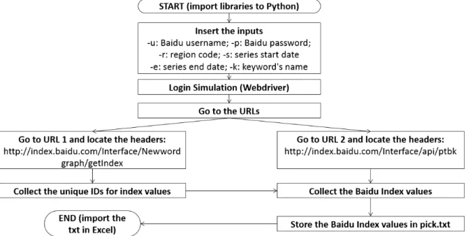
The Baidu Index time series is a challenging part for this study as Baidu only show the trend in the form of graph, and the series is not available for direct download. Users of the Baidu Index can only zoom in the graph to collect the exact time series value, which is very time-consuming. Therefore, I use Python to write a programme to facilitate the login and data extraction process. I mainly use a Web Browser Automation Module named Selenium to simulate the extraction, and the main idea of this process is explained in Appendix B.
The whole daily Baidu Index dataset starts on the first day of 2011, so I take it as the initial day of the studied period. I consider the last day of 2017 as the end of the period with the goal to gain more benefits of recent time series data compared to previous literature. Besides the period of estimation from 2011 to 2017, I use the data from 02/01/2018 to 01/07/2018 to test the forecasting power of the models.
I choose Beijing, Shanghai, Guangzhou and Chengdu to construct the panel data. These cities are the central cities of their respective regions.2 They have a large population and a higher penetration rate of Baidu. In addition, the real estate market is very active in these cities, which is suitable for a study of comparatively high-frequency real estate data. Lastly, these cities are within the first choices of the government to implement any new policies regarding real estate and therefore, the change of keyword search of the policy category is reflected in the real estate trends of these cities.
3.3 Measures of Variables
3.3.1 Time Frequency
All of the time series data is collected or adjusted into weekly. I choose this time frequency mainly to try to explore some practical implications from the Baidu Index data because the main advantage to include search engine data in real estate price or sales trend prediction is that such data from a search engine are shown in high time frequency, which means search engines update the series every day.3
2 Beijing is located in the northern part of China. Shanghai is located in the east, while Guangzhou is in the south and Chengdu is in the west.
3 On the one hand, compared to other data source, researchers may have the opportunity, in this case, to track the upcoming trend before the announcement of the new official price or transaction volume data, which generally updates monthly and nowadays only a few cities with an active real estate market have the weekly series. On the
3.3.2 Measures of the Baidu Index
In line with the outcomes from the survey, this study measures the keyword trends collected from the Baidu Index in three categories: “Housing Price” (pricing status), “Mortgage Loan” (financing) and “Purchase Restriction” (policy issues). Since each category only composites the top 5 keywords, theoretically 15 keyword trends need to be collected. However, three of the keywords in the pricing status category include the name of the studied cities, so other 9 keyword trends are collected. Additionally, I collect one more keyword because participants in the survey suggest another keyword which has the same meaning as the keyword “Affordable Housing” in the Chinese Language. Therefore, the Python programme collects in total 25 keywords trends from the Baidu Index.
The scales of the individual Baidu Index time series are different. As the study proposes a composition method based on the weights from a survey, I standardise the series by applying discrete normalisation, transforming and mapping the original data between the same range, which is 0-100 in this case before compositing the indexes.
New Index Value=Original Index Value-Min. of the seriesMax. of the series-Min. of the series ×100 (3)
I test the stationarity of these 3 composite indexes using the augmented Dickey-Fuller test (ADF) and find that these indexes do not reject the hypothesis at 5% critical value of having a unit root in the time series sample, implying that the original time series are non-stationary.4 I then further apply the log difference to obtain the growth rate of the index series during the time.
The growth of the composite indext
= ( log.composite indext/ - log.composite indext-1/ )×100
other hand, using the daily data from the Baidu Index includes many noises from the series, not being practical to predict the trend. Moreover, with weekly data chosen, the study has 1568 observations over time for each series as the total available data from the Baidu Index starts from 2011, compared to a very limited number of monthly observations.
4 Time series data require stationarity before the estimation of any predictive model to make sure the fitted model obtained through the samples can continue the pattern for a period of time in the future.
It makes the empirical results easier to interpret, and the log function also reduce the effects of excessive abnormal fluctuations and heteroscedasticity problem.5 Then I perform the ADF test again and confirm the series of the growth of composite indexes are all stationary.
3.3.3 Measures of Housing Price and Transaction Volume
I collect the weekly time series data of housing price from the CPDB directly.6 With the benefit of a much larger sample base of the second-hand apartments and a more active market, I choose the second-hand apartments weekly trends of the 4 cities in the CPDB database. It also has the advantage of fewer missing observations within the studied period. As the CPDB database only has the housing price series, I use the Choice database to get the residential housing transaction volume series of these 4 cities. I then apply the ADF test of these 8 series and find the same non-stationary situation in the original time-series. Being consistent with the Baidu Index data, I also transform these series using the log difference method and confirm the stationarities of the series of the growth rate.
3.4 Model
Considering the interdependencies of the time series, I use a Vector Autoregressive (VAR) Model for the modelling.7 Also, because of the panel data collected from 4 cities, I apply the VAR model on the stacked data. Some studies by authors such as Calomiris et al. (2013) and Haj fraj et al. (2018) define it as a penal VAR model, but the model is, in fact, a standard VAR on the stacked data, which does not apply panel estimation techniques. Compared with the panel VAR model proposed by Canova and Ciccarelli (2013), the model used in this study also exploits the benefits from a cross-sectional dimension.8 The final representation of the model is:
5 Cao and Mu (2016) also use the log terms of all the series when studying the real estate market.
6 Dong et al. (2014) document the consumer’s least attention on affordable apartments provided by the government and conclude that the second-hand apartments real estate series about pricing and transactions is similar to the one for new apartments.
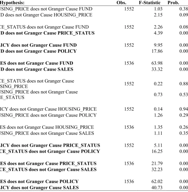
7 This paper initially refers to and modifies the ADL model for housing price and transaction proposed by Cao and Mu (2016) that considers more the time series effect However, the ADL model does not consider the interdependencies across the series. For example, the housing price in the current period is dependent on the transaction volumes of prior periods and the transaction volumes of prior periods are also dependent on the housing price before. It is because people evaluate the activeness of the real estate market not only according to the transactions but also the price. The interdependencies may also exist in the Baidu Index trend of different categories. I also run a Pairwise Granger Causality Test to see whether one series happens before another series and help predict it. The result is shown in Table 5 of Appendix D.
8 Although the model itself offers no options for fixed effects, it still uses the data in the panel to obtain the estimators. Love and Zicchino (2006) propose a methodology of the forward (Helmert) de-meaning of observations used to control for fixed effects but the econometrics behind is still under study in academia.
⎣ ⎢ ⎢ ⎢ ⎡HOUSING_PRICESALES t t PRICE_STATUSt FUNDt POLICYt ⎦⎥ ⎥ ⎥ ⎤ i = ⎣ ⎢ ⎢ ⎢ ⎡CC1 2 C3 C4 C5⎦⎥ ⎥ ⎥ ⎤ + ∑ ⎝ ⎜ ⎜ ⎛ ⎣ ⎢ ⎢ ⎢ ⎡β1,1j β2,1j ⋮ β5,1j β1,2j β2,2j ⋮ β5,2j ⋯ β1,5j ⋯ β2,5j ⋱ ⋮ ⋯ β5,5j ⎦⎥ ⎥ ⎥ ⎤ ⎣ ⎢ ⎢ ⎢ ⎢ ⎡HOUSING_PRICESALES t-j t-j PRICE_STATUSt-j FUNDt-j POLICYt-j ⎦⎥ ⎥ ⎥ ⎥ ⎤ i⎠ ⎟ ⎟ ⎞ N j=1 + ⎣ ⎢ ⎢ ⎢ ⎡ee1,t2,t e3,t e4,t e5,t⎦⎥ ⎥ ⎥ ⎤ (5)
where HOUSING_PRICE is the growth of housing price, SALES is the growth of housing transaction volume series, PRICE_STATUS is the growth of composite Baidu Index for the pricing status category, FUND is the growth of composite index for the financing category and POLICY is the growth of composite index for the policy issues category. The abbreviations of the series are also explained in Appendix C. C is the constant term and e is the error term. The index i=1,…,4 indicates each of the four different cities in the panel and j=1,…,N denotes the lag order in the model. In order to determine the lag order, I run a lag length criteria test including the Likelihood Ratio (LR), the Final Prediction Error (FPE), the Akaike Information Criterion (AIC), the Schwarz Information Criterion (SIC) and the Hannan-Quinn Information Criterion (HQ). As different criteria may suggest a different lag order, I choose the lag order that most criteria select. I use the first six months housing price and volume data of 2018 to test for the predictive power and use the following formulas to calculate the Mean Absolute Error (MAE) and Mean Squared Error (MSE) of the prediction.9
4. Results and Discussion
4.1 Results from the Survey
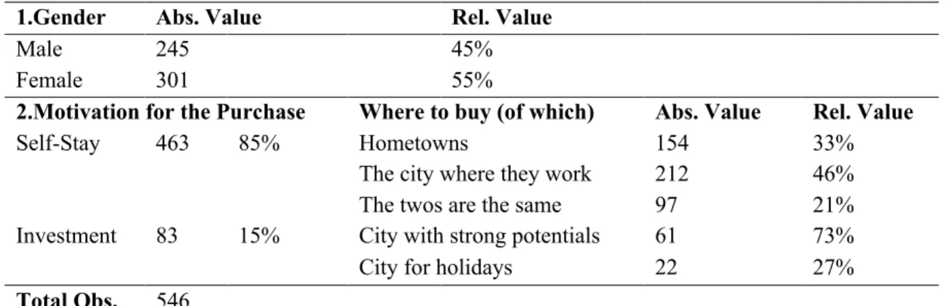
Around 45% of the participants are male and 55% of them are female. Concerning motivations, the survey separate participants into two groups: self-stay and investment. The motivation of self-stay means that these participants are going to live in the apartment after they make the purchasing decision. Although buyers with self-stay purpose also benefit from the appreciation of housing price, such income is difficult to realize compared to investors that are free to sell the apartment without finding a new one for themselves. 463 participants would like to buy an apartment for self-stay, and they prefer to buy it in the city where they work. The other 83 participants are investors in real estate, with 61% choosing to invest in a city with strong potentials, meaning that they prefer well-developed cities or cities which are growing rapidly. Table 1 shows the descriptive statistics of the survey.
9 I choose this period for forecasting because it is 1/15 of the available data. More data are used to train the model to improve the predictive accuracy because the limited numbers of data are still the main constraint.
Table 1 Descriptive Statistics of the Survey
1.Gender Abs. Value Rel. Value
Male 245 45%
Female 301 55%
2.Motivation for the Purchase Where to buy (of which) Abs. Value Rel. Value
Self-Stay 463 85% Hometowns 154 33%
The city where they work 212 46% The twos are the same 97 21% Investment 83 15% City with strong potentials 61 73%
City for holidays 22 27%
Total Obs. 546
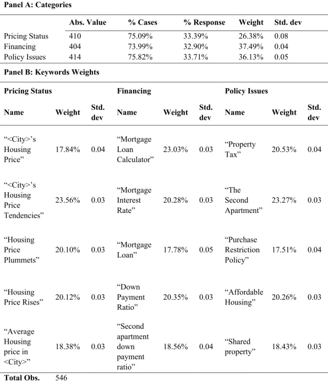
The main result of the survey is the weights that participants assign to each keyword and category. Table 2 exhibits the results of the weights of the category in panel A and the weights of keywords in panel B.
From panel A, the percentage of cases and the percentage of response of the three categories do not show a big difference, implying that people are likely to search all the three categories in general. However, people do not assign the same weight to each of them. They care more about the keyword of financing, assigning on average 37.49% and the second important category is policy issues, with a slightly lower weight of 36.13%. However, the weight for keywords of pricing status is much lower than the other two, with an average of 26.38% and the highest standard deviation. It implies that the participants focus less on keywords from the pricing status category on average, but they have more different opinions regarding the importance among themselves. An explanation for this links to the new Baidu Index observations after 2015. With the boom of the real estate market in China, the Chinese government has applied more readjustments in financing or policies. These adjustments aim to control the accelerating growth of housing price. When people concern more about the impact of these readjustments and policies, they are likely to show such a preference when searching information in Baidu.
When looking into the individual keywords from panel B, I find that people assign the weights on average between 17% and 24% and the standard deviations are comparably lower than those for the weights of categories. As no other keyword is suggested by more than 1% of participants, expect one with the same meaning but another expression in the Chinese language, the initial keyword range base on experience and previous literature covers the topic well.
Table 2 Weights of Keywords from the Survey
Panel A: Categories
Abs. Value % Cases % Response Weight Std. dev
Pricing Status 410 75.09% 33.39% 26.38% 0.08
Financing 404 73.99% 32.90% 37.49% 0.04
Policy Issues 414 75.82% 33.71% 36.13% 0.05
Panel B: Keywords Weights
Pricing Status Financing Policy Issues Name Weight Std.
dev Name Weight Std.
dev Name Weight Std. dev “<City>’s Housing Price” 17.84% 0.04 “Mortgage Loan Calculator” 23.03% 0.03 “Property Tax” 20.53% 0.04 “<City>’s Housing Price Tendencies” 23.56% 0.03 “Mortgage Interest Rate” 20.28% 0.03 “The Second Apartment” 23.27% 0.03 “Housing Price Plummets” 20.10% 0.03 “Mortgage Loan” 17.78% 0.05 “Purchase Restriction Policy” 17.51% 0.04 “Housing Price Rises” 20.12% 0.03 “Down Payment Ratio” 20.35% 0.03 “Affordable Housing” 20.26% 0.03 “Average Housing price in <City>” 18.38% 0.03 “Second apartment down payment ratio” 18.56% 0.04 “Shared property” 18.43% 0.03 Total Obs. 546
Note: 1 No other categories are suggested by the participants; 2)From the survey results, there is one another keyword suggested by the participants and it is included in "Affordable Housing" item as both of the keywords have the same meaning in the Chinese language. Other keywords suggested by the participants are answered only by 1-3 questionnaires. Those keywords like "Environment" or "Deposit Rate" are either too broad or considered to have low links with the topic both theoretically and statistically.
Additionally, another advantage of a survey-based approach is that the survey is able to separate behavioural differences in web search caused by different genders. I separate the
weights answered by different gender in the survey to see if the gender differences influence the results. Given the benefits of the survey, the study finds no major gender effect in the keywords’ selection. Only slight difference between male and female searchers are observed. Male searchers concentrate more on individual keywords like the average housing price, housing price plummets, mortgage loan, second apartment down payment ratio, shared property and purchase restriction policy. I document the relevant literature review and details of these results reported in Appendix E.
4.2 Results from the Prediction Models
The result of the lag length criteria test suggests the model of 3 lags. Table 3 shows the estimation output. The table only reports the parameters of equations with the dependent variable HOUSING_PRICE or SALES as these are the equations that give practical implications to the study. Panel A presents the results of the prediction model for housing price trend and panel B presents the results for housing transaction volume trend. Column 1 and 5 reports the model based on the survey-based composite indexes. In column 2 and 6, I model with the composite indexes assigned with equal weights. In that model, there are no relative differences in keywords weights within each category. Column 3 and 7 reports the results of search-volume-based indexes, using only the keyword series with the highest number of searches of each category in composition. Finally, column 4 and 8 present a baseline model without including any trend from the Baidu Index.
For the growth rate of housing price, unlike previous studies based on a smaller dataset, the model with the Baidu Index increase only the adjusted R2 0.285 percentage point in the survey-based model, 0.283 percentage point in the equally-weighed model and even decrease 0.234 percentage point in the search-volume-based model compared to the baseline. However, it helps justify the H1. The survey-based model has the most predictive power, also confirming the H2a. Faster growth of housing price one week before slows the growth in the current period, indicating a diminishing growth pattern of the housing price trend. For the survey-based model and the equally-weighed model, the coefficients of housing price in two and three weeks before the current period turn out to be significant positive but with less impact. The study only observes significant effects of the Baidu Index in the survey-based model and equally-weighed model, and they occur in the second lag of both the financing and the policy issues category. If the growth of searches on financing is accelerating, it reduces the growth of housing price. The impact is the opposite in the growth of searches on policy issues. When searches of this category increase, it accelerates the growth of housing price. However, the absolute values of these coefficients are comparably low.
Table 3 Prediction Model for the Housing Price and Transaction Volume Trend of Four Major Cities in China
The table presents the VARs of three different methods to composite the Baidu Indexes and one baseline model without including any Baidu Index. Appendix C contains the definition of all variables and standard errors are reported in parentheses.
Variables Panel A: housing price model Panel B: housing transaction volume model Dependent Variable: HOUSING_PRICE Dependent Variable: SALES
(1) (2) (3) (4) (5) (6) (7) (8)
Survey-based Equally-weighed Search-volume-based Baseline Survey-based Equally-weighed Search-volume-based Baseline HOUSING_ PRICE(-1) -0.198309 *** -0.197906 *** -0.187936 *** -0.200626 *** -0.706101 -0.714025 -0.621018 -0.33694 (0.02649) (0.02649) (0.02680) (0.02642) (0.66578) (0.66654) (0.65009) (0.699352) HOUSING_ PRICE(-2) 0.046865* 0.046534* 0.052909** 0.041738 -1.319519** -1.311080** -1.236173* -0.993798 (0.02698) (0.02698) (0.02724) (0.026962) (0.67811) (0.67890) (0.66075) (0.713687) HOUSING_ PRICE(-3) 0.043868* 0.043994* 0.040623 0.04107 0.564812 0.556309 0.973538 0.910018 (0.02651) (0.02651) (0.02689) (0.02647) (0.66632) (0.66712) (0.65241) (0.700652) SALES(-1) 0.000313 0.000316 0.000749 0.000414 -0.555736*** -0.553630*** -0.644054*** -0.430775*** (0.00114) (0.00113) (0.00121) (0.000982) (0.02857) (0.02856) (0.02943) (0.025985) SALES(-2) -0.000937 -0.000874 0.000199 -0.000669 -0.400001*** -0.397664*** -0.415559*** -0.295804*** (0.00124) (0.00123) (0.00134) (0.00103) (0.03110) (0.03107) (0.03242) (0.027276) SALES(-3) -0.001625 -0.001634 -0.001329 -0.001046 -0.240926*** -0.240085*** -0.255648*** -0.193091*** (0.00118) (0.00117) (0.00125) (0.000981) (0.02954) (0.02953) (0.03030) (0.025967) PRICE_ STATUS(-1) -0.002663 -0.003041 -0.003957 0.551452*** 0.551448*** 0.436774*** (0.00548) (0.00541) (0.00548) (0.13764) (0.13616) (0.13287) PRICE_ STATUS(-2) 0.003086 0.003769 0.006802 0.074066 0.096535 0.208787 (0.00560) (0.00555) (0.00557) (0.14081) (0.13972) (0.13508)
Table 3 Continued
Variables Panel A: housing price model Panel B: housing transaction volume model Dependent Variable: HOUSING_PRICE Dependent Variable: SALES
(1) (2) (3) (4) (5) (6) (7) (8)
Survey-based Equally-weighed Search-volume-based Baseline Survey-based Equally-weighed Search-volume-based Baseline PRICE_ STATUS(-3) -0.004843 -0.004761 -0.001981 0.424542*** 0.422711*** 0.407187*** (0.00546) (0.00540) (0.00546) (0.13733) (0.13588) (0.13257) FUND(-1) 0.006646 0.006332 0.007102 0.339972* 0.341623* 0.951837*** (0.00727) (0.00725) (0.00585) (0.18276) (0.18249) (0.14200) FUND(-2) -0.016518 ** -0.016724 ** -0.006840 0.996852*** 0.981006*** 0.843890*** (0.00756) (0.00754) (0.00589) (0.19009) (0.18978) (0.14299) FUND(-3) -0.004785 -0.004283 -0.004235 0.154316 0.151834 0.174723 (0.00717) (0.00714) (0.00593) (0.18014) (0.17961) (0.14380) POLICY(-1) -0.003931 -0.003658 -0.002273 0.379672** 0.371562** 0.411218*** (0.00619) (0.00612) (0.00625) (0.15567) (0.15403) (0.15159) POLICY(-2) 0.011967* 0.011146* 0.000987 0.258159 0.244794 0.154471 (0.00638) (0.00629) (0.00614) (0.16033) (0.15825) (0.14903) POLICY(-3) 0.008601 0.007949 0.005596 0.640339*** 0.632771*** 0.690181*** (0.00595) (0.00588) (0.00584) (0.14950) (0.14795) (0.14174) C 0.226623 *** 0.226672 *** 0.216477 *** 0.227763 *** -0.409112 -0.407256 0.001224 0.168976 (0.05187) (0.05187) (0.05178) (0.051828) (1.30374) (1.30514) (1.25624) (1.372783) Adj. R-squared 0.044250 0.044232 0.039054 0.041398 0.257275 0.255682 0.292267 0.174875 ***Significant at the 1 percent level. **Significant at the 5 percent level. *Significant at the 10 percent level.
Note: 1 The VAR models of 3 lags are selected based on the lag length criteria test; 2) The table only reports the parameters of equations with the dependent variable HOUSING_PRICE or SALES from each VAR model. These are the ones that give practical implications to the study.
Regarding the growth rate of housing transaction volume, the models with Baidu Index trend increase the prediction more significantly. The adjusted R2 increases 8.240 percentage points in the survey-based model, 8.081 percentage points in the equally-weighted model and 11.739 percentage points in the search-volume-based model. The results support the H1 but only partially support the H2a since the survey-based method is better than equally-based method but not better than search-volume-based method. I discuss the possible reasons in the discussion part. In these models, the housing price two weeks before have a significant negative impact on the growth of transaction volume expect the baseline model. All lags in transaction volume also have a negative impact, indicating the high activeness in sales in the past reduces the growth of sales in the current period. As for the variables of the Baidu Indexes, the study finds all significant positive effects in all of the three categories: lag 1 and lag 3 of pricing status, lag 1 and lag 2 of financing, together with lag 1 and lag 3 of policy issues. It reveals that the more activeness of searches on real estate in Baidu is linked with the more activeness of real estate market transactions.
4.3 Results from the Forecasting Test
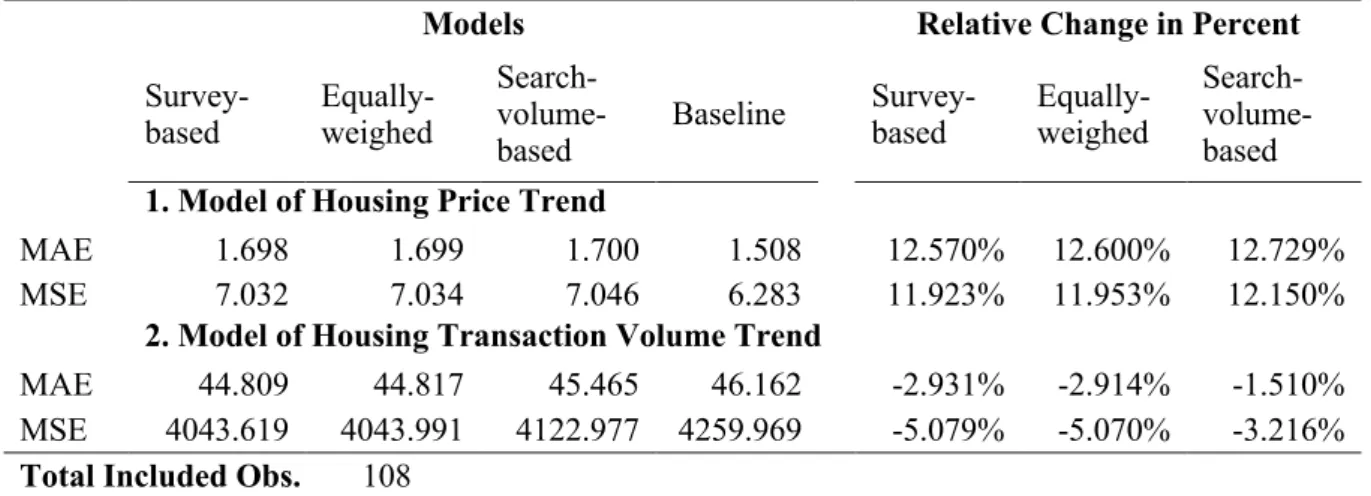
One of the main goals for a prediction model is to forecast the future. In order to test the H2b, I forecast the samples from 02/01/2018 to 01/07/2018 and calculate the MAE and MSE. Table 4 reports the results and also the relative change in percent compared to the baseline model. The negative numbers indicate the reduction of forecasting errors.
Table 4 Forecast Error Comparison
Models Relative Change in Percent
Survey-based Equally-weighed
Search-
volume-based Baseline
Survey-based Equally-weighed
Search- volume-based
1. Model of Housing Price Trend
MAE 1.698 1.699 1.700 1.508 12.570% 12.600% 12.729% MSE 7.032 7.034 7.046 6.283 11.923% 11.953% 12.150%
2. Model of Housing Transaction Volume Trend
MAE 44.809 44.817 45.465 46.162 -2.931% -2.914% -1.510% MSE 4043.619 4043.991 4122.977 4259.969 -5.079% -5.070% -3.216%
Total Included Obs. 108
The results partially support the H2b as the forecast errors are lower only in the VAR model for housing transaction volume trend. The survey-based model performs the best among the three models with the Baidu Index in this study. In the prediction model for housing
transaction volume trend, it decreases the MAE by 2.931 percent and the MSE by 5.079 percent when comparing it with the baseline model. The survey-based composite indexes also maintain the advantage in models for housing price trend. However, in this case, all the models including the Baidu Index have higher forecast errors compared to the baseline model. I discuss the potential reasons in the discussion part.
4.4 Discussion
The estimation output of this study document that the sales growth in the past do not have any significant impact on current housing price growth, while the sales growth is reduced when housing price growth accelerates in two weeks before the current period. To a certain extent, the growth of transaction volume shows the activeness in the real estate market. A real estate market is more active when there is a trend of accelerating transactions reflected in a higher growth rate in sales volume. My interpretation is that the relationship between the activeness of the market and the growth of housing price is unidirectional at least in the short-term. It is because a higher growth of housing price discourages people’s intention to make the purchase decision, but the accelerating increase of housing transactions does not cause a faster growth of housing price even though the price trend keeps growing.
Another interesting finding is that the Baidu Index does not contribute much to the housing price prediction model, but it reports a more significant impact on the models for housing transaction volume. It should be clear that housing price and transaction volume represent two completely different things. The housing transaction volume gives more implications to the activeness of the real estate market while the housing price is usually determined by the supply and demand in the market. Housing price goes up when there are fewer apartments available for sales or having more demand caused by factors like the growth of disposable income. Moreover, in China, the sudden housing price leap starting at the beginning of 2015 and the tight control proposed by the government in early 2017 are likely to distort the relationship. This reasoning may also explain the lower R2 in the models of housing price. The study has exploited different methods to minimize such distortion, and in the end, I choose to build a panel with the most representative cities, with the objective to have more observations in the study.
When looking at panel B of Table 3, we notice different lags structure of significance in different categories. For the category of pricing status and policy issues, one week and three weeks before the current period are significant while for the category of financing, only the values with the two-week lag have the highest significance level. With this result, it helps separate the effects from different categories and has implications for short-term prediction.
For example, if a sudden accelerating growth happens in keywords of pricing status and policy issues category from the Baidu Index, researchers are likely to observe the growth rate for the housing transaction volume will accelerate in the following week. If the growth rate of financing category one week before the current period also increase, that probability is even higher.
After comparing my results with the results in previous literature, all the R2 of the models in this study seems quite low. For the housing price model, they are less than 0.044 and for the housing transaction volume model, the number is less than 0.292. One may ask whether the proposed model has practical meanings in real estate trends prediction. One possible reason is that I adjust all the time series into the growth rates when dealing with the stationarity problem and a well-built model for real estate prediction should not only include the online search patterns and the housing price or transaction volume trends in the past. Second, the high time-frequency of the time series data may have an impact on the overall model performance since a higher time-frequency also means more noises in the series. However, the Baidu Index is only available from 2011 and taking the complexity of characteristics in Chinese cities into account, the weekly time series is the most reasonable choice and fits in with the goal of exploring some practical implications from higher time-frequency data on real estate in this study. Moreover, I observe from Table 3 the R2 of the baseline model is also low. A possible explanation for this low R2 is the possible distortion already mentioned in the new dataset. Yet, it should be mentioned that the goal of this study is actually to explore if a survey-based approached is an alternative for index composition and it has already shown better performance compared to the alternative methods. Therefore, the survey-based approach is applicable for research of this kind.
Since in the literature the correlation-based composition methods vary and are not specified in previous studies, I am not able to replicate the process to compare it with the survey-based method. However, I have reservations whether the decomposition method based on the higher absolute value of correlation coefficients also results in outputs of higher levels of significance when modelling. Also, I observe a non-linear relationship in the patterns between the original Baidu Index series and the real estate trends, so a suitable measure of dependence may not always be such correlation coefficients. In the first stage of selection, the correlation coefficients may help to eliminate keywords without any links with the dependent variables, but assigning weights using these coefficients seems hard to be explained.
The first inconsistency with the hypotheses is that the search-volume-based model has higher R2 than the survey-based model in comparisons of different composition methods of the Baidu Index, in panel B of Table 3. However, the higher R2 does not mean that the
search-volume-based method is generally better than the survey-based method as R2 is only one of the indicators. To explain this, the main difference of significance levels in parameters between these two models lies in the 1-lag coefficient of the financing category’s composite index growth. That coefficient is significant at the 1 percent level in the search-volume-based model while in the other two models it is only significant at the 10 percent level. The keyword representing the financing category in the search-volume-based model is “Mortgage Loan Calculator”, which searchers are believed to search in a shorter term compared to other keywords in the same category. It is because other keywords like “Mortgage Interest Rate” or “Down Payment Ratio” are the inputs to insert in the calculator and people can only calculate their monthly payments after they have these inputs in their hands. More importantly, before signing the contract, people tend to search such a calculator to confirm how they are going to pay. Therefore, assigning the calculator keyword with the weight of “1” are likely to increase the significance of a shorter lag. Since the composite index representing the financing category should be more comprehensive and in comparison with the forecast errors, the survey-based method outperforms the other two models. Besides, the survey-based method has the unique advantage of possessing empirical supports from searchers’ answers while the possible explanation above relies only on logical reasoning. However, this result offers some new insights for the prediction model using the higher frequency data: keywords within a certain category may also have different lag structures and it could be a good direction for future studies when a more extended period of the time series is available.
The results report the other inconsistency with the hypotheses in the forecast errors of housing price trend models. For housing price trend, all models including the Baidu Index have higher forecast errors ranging from 11.923 percent to 12.729 percent if I compare them with the baseline model. Under the same prediction methodology, such a result may be caused by having a lot of insignificant parameters in models with the Baidu Index. These insignificant variables have a negative impact on the forecasting power. However, even though all models for housing price trend with the Baidu Index underperform the baseline in forecast errors, the survey-based model has the lowest increase among the three alternative ways of composition. It may still imply that using the weights from a survey is better to composite the Baidu Index.
5. Conclusion
This study examines the effect of composite Baidu Indexes, weighed using a survey-based approach, on the prediction of the housing price and the housing transaction volume in China. Having its root in 546 surveys and weekly panel time series of four major Chinese cities generated from 25 individual keywords and 8 real estate trends from 2011-2017, I find that the
survey-based composite indexes contribute and outperform the equally-weighed methods and the search-volume-based methods, especially in the prediction model of housing transaction volume. The survey-based indexes also lower the forecast errors in the prediction model of housing transaction volume. The majority of these findings are consistent with the hypotheses except for a higher R2 in search-volume-based indexes for transaction volume and the higher forecast errors in models with the Baidu Index for housing price trend. Furthermore, I find no major difference between the weights from male searchers and female searchers, but they show a slight difference in preference for some individual keywords.
The paper has some implications. Firstly, it provides empirical supports of searcher’s behaviours by conducting a survey to composite different individual Baidu Indexes. The survey reports that people on average assign similar weights to each individual keyword they want to search and there is no significant gender difference. Both of them imply the reasonability of using assigned weights from the survey in composition. Secondly, it exploits the interdependency of variables by using a VAR model and reconfirms the predictive power of the Baidu Index with the new data in which a booming of real estate market and strong readjustments from the government have happened. Thirdly, it enhances the understanding of the relationship between real estate trends and search engine data, especially in a higher time-frequency compared to previous studies.
Although the study sheds some light on a new keyword selection approach, there are some limitations. For instance, the survey may not fully reflect the overall situation of people’s idea towards different individual keywords because of the limited research resources. The design of the questions still has some room for improvements as the allocation of points in the survey may be difficult to make the weights sum up to 100 points. I observe in the survey results that some participants assign a few points in “Others” keyword but do not specify them with their new keywords. Moreover, a larger sample base for the survey and better randomisation are always preferred.
In terms of limitations in composition, my findings suggest that taking the different lag structures among the individual indexes into account is likely to change the performance of the composite indexes. In this study, I do not have enough information to lag some of the individual indexes before applying the composition formula because in that case, an additional question in the survey may be added to ask the search order of keywords and the time of being searched. Additionally, in the stage of VAR models, the model does not contain restrictions on the VAR coefficients matrix which may potentially influence the final results. It is for sure that in future studies more related variables can be added as control variables.
Even though the study reveals some benefits of the survey-based keyword selection approach and shows the predictive power of the Baidu Index to real estate trends in a higher time-frequency level especially for housing transaction volume trend, some improvements are available for future research. First of all, the lag structure of individual indexes combined with the survey approach is an interesting direction to explore the contribution of search engine data for prediction further. Secondly, discovering more sophisticated related factors in high time-frequency is beneficial for a study in this kind. These factors can be included in the model to increase the model’s predictive power. Besides, the noise in higher time-frequency time series reduce the accuracy of prediction, so future studies may elaborate a better process to filter out irrelevant information from the search engine indexes on real estate.
References
Bai, L., & Yan, X., & Jin, J. (2015). Forecast the Commercial Housing Price Index Based on Search Keywords Attention. Forecasting, 34(4), 65-70.
Calomiris, C., Longhofer, S., & Miles, W. (2013). The foreclosure-house price nexus: A panel var model for u.s. states, 1981-2009. Real Estate Economics, 41(4), 709-746. doi:10.1111/reec.12011
Canova, F., & Ciccarelli, M. (2013). Panel Vector Autoregressive Models: A Survey.Working Paper Series (European Central Bank), no. 1507,205-246.
Cao, X., & Mu, H. (2016). Prediction Research on Commercial Housing Sales Volume Based on Web Search. Construction Economy, 37(2), 73-77.
Case, K. E., & Shiller, R. J. (1988). The behavior of home buyers in boom and post-boom markets.
Case, K. E. & Shiller, R. J. (2003). Is There a Bubble in the Housing Market? Brookings Papers
on Economic Activity 2003(2), 299-362.
Daniel, W. W., & Cross, C. L. (2018). Biostatistics: a foundation for analysis in the health sciences. Wiley.
Dong, Q., & Sun, N., & Li, W. (2014). Real Estate Prediction based on Web Search Data.
Statistical Research, 31(10), 81-88.
Glaeser, E. L., Kim, H., Luca, M., & National Bureau of Economic, R. (2017). Nowcasting the local economy: using Yelp data to measure economic activity NBER working paper
series; no. 24010; Working paper series (National Bureau of Economic Research); no.
24010., Retrieved from http://www.nber.org/papers/w24010
Haj fraj, S., Hamdaoui, M., & Maktouf, S. (2018). Does regime choice affect exchange rate volatility-economic growth link? an application of panel-var approach. International
Economic Journal, 32(1), 1-30. doi:10.1080/10168737.2018.1423627
Hong, T., & Li, W. (2015). A Study on the Relationship Between Expectation and Real Housing Prices Based on Query Index. Statistics & Information Forum, 30(11), 49-53. Huang, X. K., Zhang, L. F., & Ding, Y. S. (2017). The Baidu Index: Uses in predicting tourism
flows -A case study of the Forbidden City. Tourism Management, 58, 301-306. Jiang, W., Lai, Y., Wang, K. (2016). Research on the correlation of real estate prices based on
Baidu Index. Statistics and Decisions, 2016(2), 90-93.
Koohang, A., & Durante, A. (2003). Learners' perceptions toward the web-based distance learning activities/assignments portion of an undergraduate hybrid instruction model.
Kulkarni, R., Haynes, K. E., Stough, R. R., & Paelinck, J. H. (2009). Forecasting housing prices with Google econometrics.Social Science Electronic Publishing.
Large, A., Beheshti, J., & Rahman, T. (2002). Gender differences in collaborative web searching behavior: an elementary school study. Information Processing and
Management, 38, 427-443.
Liu, C., Zhou, Y., Zhao, W., Jiang, Q., Liang, X., Li, H., . . . Fan, S. (2018). Performance Evaluation of Housing Price Regulation Policy in China: Based on ARIMA Model and Intervention Analysis Proceedings of the Eleventh International Conference on
Management Science and Engineering Management, 1773-1785.
Liu, T.-Y., Chang, H.-L., Su, C.-W., & Jiang, X.-Z. (2016). China's housing bubble burst?
Economics of Transition, 24(2), 361-389.
Love, I., & Zicchino, L. (2006). Financial development and dynamic investment behavior: Evidence from panel var. Quarterly Review of Economics and Finance, 46(2), 190-210. doi:10.1016/j.qref.2005.11.007
Lütje, T., & Menkhoff, L. (2007). What drives home bias? Evidence from fund managers' views. International Journal of Finance & Economics, 12(1), 21-35.
Pan, B., Chenguang Wu, D., & Song, H. (2012). Forecasting hotel room demand using search engine data. Journal of Hospitality and Tourism Technology, 3(3), 196-210.
Park, B., & Bae, J. K. (2015). Using machine learning algorithms for housing price prediction: The case of Fairfax County, Virginia housing data. Expert Systems with Applications,
42(6), 2928-2934. doi:10.1016/j.eswa.2014.11.040
Pu, D., & Shao, D., & Wu, T., & Zeng, J., & Qian, W. (2018) Housing Price Prediction based on Web Search Data. Information & communications, 181, 17-19.
Roy, M., & Chi, M. T. H. (2003). Gender differences in patterns of searching the Web. Journal
of Educational Computing Research, 29(3), 335-348.
Schumacher, P., & Morahan-Martin, J. (2001). Gender, Internet and computer attitudes and experiences. Computers in Human Behavior, 17(1), 95-110.
Shang, X., & Qiu, P. (2008). On the Online Marketing with the Real Estate Brand. Reformation
& Strategy, 7(24), 125-128.
Tsai, M. J., & Tsai, C. C. (2010). Junior high school students' Internet usage and self-efficacy: a re-examination of the gender gap. Computers & Education, 54, 1182-1192.
van Dijk, D. W., & Francke, M. K. (2017). Internet Search Behavior, Liquidity and Prices in the Housing Market. Real Estate Economics.
Vaughan, L., & Chen, Y. (2015). Data Mining From Web Search Queries: A Comparison of Google Trends and Baidu Index. Journal of the Association for Information Science
and Technology, 66(1), 13-22. doi:10.1002/asi.23201
Wang, X., & Wei, W. (2015). Resident's Limited Attention and Housing Bubble: General Empirical Mode Decomposition Taking Baidu index as Attention. Commercial
Research(3), 79-83.
Wu, J., & Deng, Y. H. (2015). Intercity Information Diffusion and Price Discovery in Housing Markets: Evidence from Google Searches. Journal of Real Estate Finance and
Economics, 50(3), 289-306. doi:10.1007/s11146-014-9493-9
Wu, L., & Brynjolfsson, E. (2015). The Future of Prediction: How Google Searches Foreshadow Housing Prices and Sales. NBER Chapters, 147.
Yang, S.X., & DONG, J.C., & Li, X.T. (2013). A Study of Factors Influencing Real Estate Price Based on Network Keywords Search. Journal of Xinjiang University of Finance
and Economics, 56(3), 5-12.
Zhou, M. (2014). Gender difference in web search perceptions and behavior: Does it vary by task performance? Computers & Education, 78, 174-184.