Finance from the NOVA – School of Business and Economics
Intraday Volatility Estimation in High-Frequency Data Using
Order Book Information
Jules William Rudolf Netze (30290)
A Project carried out on the Master in Finance Program, under the supervision of:
Paulo M. M. Rodrigues
Lisbon, 3rd of January 2019
Abstract
This research conducts high-frequency intraday volatility estimations on the Euro Stoxx 50 Future under the multiplicative component GARCH framework, where the conditional volatility of high-frequency returns is decomposed into a daily, diurnal and stochastic intraday component. In contrast to existent research, this research covers a relatively long period of 423 trading days corresponding to about 345,000 1-minute observations. This study reveals that return series derived from the Limit Order Book have superior model features compared to simple trade returns. We find that these returns overcome the shortcomings of the well-documented microstructure noise. Standardized residuals follow a white noise process and follow more closely a normal distribution compared to simple trade returns. However, this comes at the cost of larger coefficient instability and larger outliers in the estimated residuals. KEYWORDS: GARCH, volatility estimation, high-frequency data, limit order book.
1. Introduction
In financial markets high-frequency trading plays a significant role in price discovery and liquidity provision according to recent literature (see e.g. Bouveret et al. (2014)). Jarnecic and Snape (2014) found that market makers provide small but stable liquidity on the lower levels around the best bid and ask price and earn the corresponding spread as a profit. Arbitrageurs use high-frequency algorithms to discover price inefficiencies across markets and securities and will exploit the inefficiency until it converges to its fundamental price again. The vast majority of recent literature covered the topics of price discovery and discussed if high-frequency trading contributes to it. Another stream of literature focused on the ability of intraday volatilities to model better and more accurate end of day volatility estimates that serve as an input for several risk applications. However, only little research has been done to uncover the predictability of spot (intraday) volatility. High-frequency trading strategies rely heavily on the expected future spot volatility, as an input parameter for algorithms to place limit orders or to schedule trades. The existing research on this topic is mainly focused on equities. However, we find that there is the need to extent the research to equity benchmark futures as they have far reaching applications in financial markets. They serve as a financial instrument to control for stock exposure in portfolio management and are used as a hedging instrument for option trading. As market participants only have to deposit a margin to trade futures, they are far less capital intensive compared to a replicated cash basket. Moreover, most of the current research covers only a relatively little time period (between 3 to 4 months of trading data) as historic intraday data is rarely available and computational expensive. Our data set covers data of almost two years of trading and therefore delivers robustness against seasonality effects and can also capture the effect of structural changes in trading sentiment. We unveil that incorporating information from the Limit Order Book (LOB) enhances model specification. This comes at the cost of larger time-variation in the coefficients and extreme outliers in the standardized residuals, which are likely to be induced by the seasonality of liquidity and shocks
in liquidity occurring in the LOB.
This paper is structured as follows. The first section provides a literature review on three different topics that are covered in our research. The first topic provides an overview on research that analysed the implications of dealing with high-frequency data. The second topic covers research that has been done on the informational content of the LOB. The last topic is about research focused on intraday volatility modelling. In Section 3, we discuss our data set, while providing general information about the Euro Stoxx 50 Future (FESX) market. In section 4 we introduce our model and the constructed prices from the LOB. In section 5 parameter estimation and an extensive property analysis is presented. The final section provides our conclusion.
2. Literature Review
2.1. High Frequency SamplingThe rise of high-frequency trading has flooded financial markets with large amounts of data recorded up to nanoseconds. Nonetheless, the majority of academic work suggests high-frequency data to be sampled at an arbitrary high-frequency of 5-minutes such as Anderson et al. (2001) and Liu et al. (2015). This results in much of the data being discarded from the analysis. The main reason for this low frequency sampling is due to the presence of market microstructure noise in high-frequency data. Microstructure noise refers to the bid-ask bounce, discreteness of price change in markets that are not decimalized, latency in representativeness of price changes and informational asymmetries among traders. Zang et al. (2005) argue that price series observed over a short time interval are mainly composed of shocks stemming from microstructure noise and reveal little about the true volatility of the price process. Assuming the amount of market microstructure noise remains constant at different frequencies, the volatility obtained by price series sampled at lower frequencies contains less microstructure
of the price process. In more statistical terms, high-frequency price return series tend to experience a high degree of autocorrelation. This persistent memory is what leads to a highly biased estimation of the variance, when calculated as the sum of the squared returns as stated by Gatheral and Oomen (2010).
To correct for these microstructure effects Gatheral and Oomen (2010) suggest using, instead of transaction prices, volume weighted mid-quote prices, also called micro prices. ‘The
micro-price, more familiar to practitioners, linearly weighs the bid and ask prices by the volume on the opposite side of the book and thus can be interpreted as the market clearing price when demand and supply curves are linear in price.’ (Gatheral and Oomen, 2010, p.5)
They show that micro price return series suffer far less from autocorrelation than transaction price return series due to the reduction in the microstructure noise based on simulated data. This property makes them more suitable for sampling at higher frequencies. However, Stoikov (2017) argues that the micro price, as calculated by Gatheral and Oomen (2010), has several shortcomings. The first one is that the order book receives updates every few nanoseconds, assuming a highly liquid market, which leads to continuously changing micro prices. This may lead to noisy volatility estimations for micro price series. Secondly, the micro price lacks theoretical justification for being the ‘fair’ price of a specific asset, since the micro price is not necessarily a martingale. Stoikov (2017) proposes a micro price, which is constructed as a martingale, conditional on the information in the LOB, such as the bid-ask spread and the order book imbalance.
2.2. Limit Order Book Information
The before mentioned micro prices incorporate information from the LOB. The LOB is basically a decentralized database, which was first proposed by the U.S. Securities and Exchange Commission (SEC) in the early 2000’s. Since then its popularity surged and throughout the years it has become a central part of the global financial market structure. A
LOB system allows its users to view and place orders at a number of price levels away from the best ask and bid price. For each price level the order book displays its price and corresponding quantity. Market participants can either enter a market order which will be executed instantaneously at any given price, whereas a limit order sets the maximum (minimum) price someone is willing to buy (sell), but execution is not guaranteed. The question in current academic literature remains whether these different levels actually reveal any relevant price information beyond the first level.
Cao et al. (2004) hypothesize that the limit orders after the best bid and ask price contribute to price discovery. The shape of the order book gives traders a useful overview of the current demand and supply in the market. Especially, the imbalance on the ask and bid side of the LOB indicates shifts in the supply and demand curves. Their empirical evidence suggests that the order book beyond its first step is moderately informative and the information share beyond the first level is around 22%, where the highest contribution stems from the fifth level up to the tenth level of the LOB.
Rock (1996), Angel (1997) and Harris (1998) argue in their theoretical LOB models that informed traders, who obtain short-lived private information, would prefer a market order to a limit order due to its immediate execution. This implying that traders mainly make use of market orders. In contrast, Anand et al. (2005) find empirical support for informed traders’ use of limit orders. They examine the relative use of market orders versus limit orders by informed and liquidity traders during the day using detailed order and audit trail data from the NYSE for 144 stocks. In their research, institutional traders are classified as informed traders and individuals as uninformed traders. They find that informed traders actually use a combination of market order and limit orders, where market orders are preferred in the first half of the day and limit orders in the second half. Furthermore, limit orders placed by informed traders perform better than limit orders placed by uninformed traders.
2.3. Intraday Volatility
The rise in high-frequency trading has also driven interest in modelling the volatility of those high-frequency price return series. In other words, the modelling of intraday volatility. One of the main issues related to intraday volatility modelling is intraday seasonality. This relates to the U-shape that is often observed in the daily volatility pattern. This pattern can be explained by global trade activity, implying financial products that are continuously traded and is mainly due to the opening and closing hours of financial centres at different moments of the day. In the morning, around opening time, most market traders place their orders causing a subsequent increase in the volatility of that specific securities market. The following hours volatility decreases smoothly due to less activity in the market with the lowest activity normally observed during lunch time. The second spike is usually detected when another large financial centre starts trading, such as the American or European market. When the traders of that specific opening market start placing their orders is the moment when the second spike in the volatility occurs. This recurring pattern causes the return volatility to have a slow decay in autocorrelation coupled with a strong daily conditional heteroskedasticity (Anderson and Bollerslev, 1997).
In the literature there have been many attempts to resolve the issue of intraday seasonality sparked by diurnal trading activity patterns. Anderson and Bollerslev (1997) in their attempt to model the volatility of five-minute returns of exchange rates, build a multiplicative model of daily and diurnal volatility. In their paper the conditional variance is expressed as a product of daily and diurnal components. They estimate the diurnal pattern by a Fourier flexible functional form. Anderson and Bollerslev (1998) extend their previous model by adding a dummy variable which should be able to capture the effects of macroeconomic announcements on the volatility. This approach of capturing daily effects has generally been used in the literature. Nonetheless, Engle and Sokalska (2012) argue that adding a dummy variable associated with a particular announcement is not very practical, especially
when modelling a large number of stocks. They argue that the majority of these macroeconomic announcements occur before markets open and that the consequent reaction of the market heavily depends on whether the news was genuinely expected or not. Furthermore, markets are more prone to shocks coming from asymmetric information among market participants. Engle and Sokalska (2012) propose a GARCH with a multiplicative component, which specifies the conditional variance to be the product of daily, diurnal, and stochastic intraday volatility. For the daily variance component, they make use of commercially available volatility forecasts, such as volatility forecasts derived from a multifactor risk model. The diurnal variance pattern is computed by dividing the variance of returns, by the daily variance forecast. Throughout the years the literature has mentioned several alternative ways to capture the diurnal pattern. Engle and Sokalska (2012), compared to Andersen and Bollerslev (1997), apply a more simplistic approach to calculate the diurnal pattern, which allows its daily shape to take on any form. The last step of their model is to normalize the stochastic component, the error term, by dividing it by the diurnal pattern and the daily volatility forecast. In their paper the model is used to forecast the volatility of 10-minute returns of 2,500 US stocks. Their research concludes that the addition of a new stochastic intraday component produces better volatility forecasts than the GARCH model with solely diurnal and daily components.
3. Market Environment, Data and Stylized Facts about the Limit
Order Book
3.1. The Euro Stoxx 50 Market
The Euro Stoxx 50 Future (FESX) is a future contract on its underlying cash index, a market capitalization weighted stock index, comprising the 50 largest publicly traded companies within the Eurozone. The FESX Future has quarterly expirations, namely in March, June,
month. If this is not a trading day, then it is the exchange day immediately preceding that day. The future is a cash settled instrument, meaning at expiration a seller or buyer receives/pays the difference between the initial trade price and the final settlement price. The tick size of a contract is 1 index point and is valued 10€/point. The minimum quote size for market makers is 10 contracts on the bid and ask side. The maximum spread is 1 index point. In a fast market environment, where market participants find eased quoting rules, the minimum quote size is reduced by 50% and spreads can increase by 100%. Fast markets are set by Eurex’s market supervision in general before scheduled economic releases. Market makers have a minimum quote duration of 70% of the trading hours between 09:00 and 17:30 CET (on a monthly average) (Eurex Exchange - Matching Principles, 2018). Nevertheless, excluding the opening and closing auction, the FESX Futures are open for trade from 08:00 until 22:00 CET.
A core element of the Eurex market model is the central order book (T7). During a trading day all orders and quotes are entered in this order book, except those entered via TES (Trade Entry Services). Those orders and quotes are sorted by price, type and entry time. Quotes and limit orders are sorted together. Market maker quotes are not specially considered. Equity futures follow the matching principle, better known as the price-time priority. This principle is applied to quotes and orders. When entering an order in the order book it receives a time stamp. By prioritizing orders with same price but earlier timestamp one or more transactions are generated if there are matching contrary orders. For the matching process, T7 treats orders and quotes identically. Therefore, in the following, the term “order” is generally applied to both orders and quotes. With 1,200,000 traded contracts on average a day in 2018 (Eurex Exchange - Trading Statistics, 2018), the FESX is one of the most liquid products of the Eurex Exchange.
3.2. Data
The sample period includes trading days from January 3, 2017 to September 28, 2018 resulting in 444 trading days for analysis. The research focuses on the actively traded future contract (front month). Taking the impact of rollovers into consideration, observations two days prior to an expiration date are excluded. Furthermore, the 12th of September was deleted from the analysis as the file contained errors.
This leads to a final data sample of 423 trading days. The order book data comprises every tick order with prices and sizes up to the 10th level for the bid and ask side including a timestamp, traceable up to nanoseconds. The trading data includes every trade with a timestamp, its executed price, traded volume and the side that initiated the trade (buy/sell). Intraday timespan are open market hours from 08:00 until 22:00 CET, excluding the opening and closing auction. The initial dataset (tick-by-tick) is 150 GB. Python was used to reconstruct the order book in a format such that it can be analysed for statistical purposes. For statistical analysis we used R. We decided to subsample at 1-minute intervals, resulting in 344,449 observations during our sample period. Although we would like to analyse the data at higher frequencies the computational requirements are not met.
3.3. Stylized Facts about the Euro Stoxx Future Limit Order Book
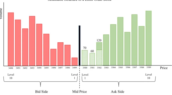
In a LOB every market participant can enter his orders. Orders can be either sell (bid) orders or buy (ask) orders. As market participants do not necessarily want to buy or sell an asset at the current observed price, but somewhere close to this price they can enter limit orders. A trade will be executed once an order of the opposite direction is entered at the limit. As many participants enter such limit orders with the corresponding quantities, they are willing to buy or sell at a given price, the order book can be aggregated across price levels. Figure 1 shows a schematic structure of a LOB.
Imagine, someone wants to buy 200 contracts, but is not too concerned about price execution and therefore enters a market order. At a given point in time (ceteris paribus) the price level of 3,500 contains only 70 contracts to buy and thus the price will increase to 3,501 with still 130 (200 – 70) contracts to buy. As this level (3,501) only contains 60 contracts the price will jump one more level up to 3,502 and will remain at this level as the market order (200 contracts) is filled (50 contracts will remain at price 3,502).
Figure 1 – Schematic Illustration of a LOB
If someone would have entered this order with a price limit of 3,501 only 130 contracts would have been traded (Level 1 and 2).
The FESX Future is a highly liquid market in many aspects. Over the sample period we find that spreads stayed at minimum tick (1 basis point) for 99.2%. Order book depth, defined as the cumulative volume of contracts across bid and ask levels displays intraday seasonality (Appendix Figure 1). In the morning hours of trading, market participants start to actively place limit orders and the order book gets filled. During the day you see an increase in order book volume, which is decreasing significantly around 17:30 when the cash market in Frankfurt closes. In the late evening hours, market participants start to cancel their remaining orders in the book leading to slow decrease in order book volume until the Futures exchange closes. For
3509
Bid Side Ask Side
V olume Mid Price Level 10 Level 10 Level 1 Level 1 3499 3498 3497 3496 3495 3494 3493 3492 3491 3490 3500 3501 3502 3503 3504 3505 3506 3507 3508 Price 70 60 120
descriptive statistics about the order book and trade data over our sample period see Appendix Table 1.
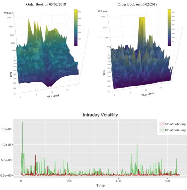
The order book is very sensitive to news impacts and the agreement upon a fundamental/fair price of the FESX Future at a given point in time (see Figure 2 for an illustration of the order book for two consecutive days). February 5, 2018 can be defined as a “normal” trading day, where at the best bid and ask level (in Figure 1 this is level 9 and level 10 respectively) most of the trading occurs, as characterized through a clearly shaped valley along the trading day. This occurs since market makers are active at these levels, contributing with stable, but small liquidity (volume). In the higher levels more liquidity can be found, as “hedgers” and “speculators” place their limit orders here. Hedgers tend to trade larger sizes to neutralize option delta or other offsetting positions. Speculators, in fact, want to gain or reduce market exposure as they believe that markets are on the rise or declining. Both are concerned about price execution and therefore place limit orders instead of market orders. However, large sizes tend to be traded using the TES (Trade Service Functionality), where two or more market participants agree upon a price for a trade. Trades in the TES system do not appear in the LOB. In turbulent market times, the order book does not have this structure anymore. On February 6, European markets were hit by the “short vol-squeeze”, caused by a sharp decline in the S&P500 and a spike in the VIX the evening before. The line chart in Figure 2 shows the realized spot volatility for the given days. One can clearly see, that volatility during February 6, 2018 exceeded the one observed during February 5, 2018 by far.
Figure 2 – Intraday Order Book and Volatility for the 5th and 6th of February 2018
As seen in Figure 2 the order book has random “volume” spikes concluding that market participants do not agree upon a fair price level. During such times, market makers and other high-frequency participants normally step out of the market, as they do not like excessive volatility (Easley et al., 2012).
4. Methodology
To estimate and forecast volatility in high-frequency data one needs to take into consideration several features of intraday returns, such as microstructure noise, the well-known intraday
Order Book on 05/02/2018 Order Book on 06/02/2018
Ti m e Ti m e Volume Volume
seasonality and the discreteness of the underlying price for FESX Futures, which has the minimum change of 1 index point by construction.
As previously discussed, recent literature (Liu et al., 2015) suggests to sub-sample intraday returns at a frequency between 5 to 10 minutes. In liquid markets, such as the FESX market, this would mean 99.7% of the observations (341 trades) would be lost for trade data on a randomly chosen day (20/02/2017 from 10:30 until 10:35), when sub-sampling at 5-minutes intervals. The loss is even larger when considering order book updates. Within the mentioned time interval there were 10,048 updates. Due to the nature of the FESX market (a lot of market makers, institutional traders and arbitrageurs) it would be naïve to believe that observations at higher frequencies do not contain any information about price formation in the market.
In the following section the model setup and the incorporated model assumptions to overcome the aforementioned features of high-frequency returns are explained in detail.
4.1. Notion
In the following, observation days are indexed by 𝑡 (𝑡 = 1, … , 𝑇). Each observation day is subsampled into 1-minute intervals, where always the last available price for a particular bin was used. Intraday data is denoted as 𝑖 ( 𝑖 = 1, … , 𝑁), i.e., a price for the FESX Future for a given day and time is expressed as 𝑃-,.. Continuous price returns are then calculated as,
𝑟-,. = ln 3 45,6
45,6789 for 𝑖 ≥ 1. (1.0)
The analysis follows the convention as in Engle and Sokalska (2012) who suggest to leave-out over-night returns, where implications will be discussed in detail later. Furthermore, for some time intervals there was no trade data available due to the fact that no trade was executed within a 1-minute interval. This occurred especially in the evening hours. For estimation and
comparison those observations are deleted, leading to 344,449 1-minute bins during the sample period.
4.2. The Model
The paper follows closely the proposed multiplicative component (mcs)GARCH framework used in Engle and Sokalska (2012) with minor adjustments proposed by Ghalanos (2018), by decomposing the conditional variance of intraday returns as a product of stochastic intraday volatilities, and diurnal and daily components. The process of intraday returns can thus be expressed as:
𝑟-,. = 𝜇 + 𝜀-,. (2.0)
𝜀-,. = >𝜎-,.ℎ-𝑠.B 𝑧-,., (2.1)
where
𝜎-,., is the stochastic intraday volatility;
ℎ-, is a proxy for the forecasted daily end of day volatility;
𝑠., the diurnal pattern for each intraday interval;
𝑧-,., is the i.i.d. (0,1) standardized innovation that follows a student-t distribution. This paper finds that trade price returns as well as returns of the latent prices are leptokurtic and fat-tailed distributed (Appendix Figure 2). Thus, in estimation we assume a student-t distribution for the conditional distribution to try to capture most of these properties. In contrast to Gatheral and Oomen (2010), we do not find that any of the return series suffers from strong autocorrelation (Appendix Figure 3).
The daily forecast for 𝜎- is derived from implied option volatilities on the FESX Future. The one day lagged VSTOXX Index, a benchmark index for implied option volatility on the
FESX Future, thus serves as a forecast for the expected end of day volatility. As the VSTOXX is expressed in annualized terms this research uses market convention - the square root of 260 trading days - to come up with a daily volatility estimate. Busch et al. (2011) find for different asset classes that ‘implied [option] volatility contains incremental information about future
volatility’ (p.1) and serves as an unbiased estimator for 2 out of 3 investigated asset classes,
namely the FX and Stock market. If in our case the implied volatility on the FESX Future serves as an unbiased estimator for future realized volatility, and we assume the intraday returns to be serially uncorrelated, then the daily conditional variance is nothing else than the sum of the squared returns of each 1-minute interval. Thus,
𝐸 3∑ F5,6G
H5
I
.JK 9 = 𝜆, (2.3)
where 𝜆 is a fixed constant.
If overnight returns are included and the mentioned assumptions hold, 𝜆 should equal to one. If the estimate is biased but constant over time, then 𝜆 will be a value different from one. However, this will not affect the subsequent model. Using this parsimonious approach, daily forecasts over longer time horizons for the multiplicative component GARCH model are not necessary and one can work with shorter samples (Engle and Sokalska, 2012). The diurnal component of the described process can be expressed as follows,
𝑠. = 𝑚𝑒𝑑 3PQ5,6G
H5G9, (2.4)
where 𝜀̂-,. is the actual residual of the estimation.
We thus obtain the normalized residuals by dividing the residuals by the diurnal and daily volatility, i.e.,
𝜀̅-,. = PQ5,6
which are then used to estimate the stochastic volatility component 𝜎²-,. following a plain
GARCH(1,1) model, such as 𝜎-,.V = 𝜔 + ∑ 𝛼
Y Z
YJK 𝜀̅²-,.[Y+ ∑]YJK𝛽Y𝜎²-,.[Y. (2.6)
Deviating from Engle and Sokalska’s (2012) approach, the conditional mean as well as the variance equation are jointly estimated. Moreover, this approach uses the median instead of the mean for the diurnal component as it is found to be more robust (Ghalanos, 2018).
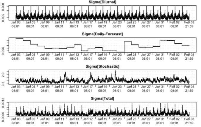
We estimated different GARCH model specifications with different lags in 𝑞 and 𝑝. Nevertheless, depending on the latent price variable we find that a parsimonious specification i.e., (p=q=1) is generally enough, as the return series do not show large memory effects, beside outliers (Appendix Figure 3). Furthermore, Figure 3 shows the volatility decomposition into the diurnal pattern, the stochastic volatility component and the daily end of day forecast from January, 3 2017 until February, 3 2017 for trade returns.
Figure 3 – Decomposition of total volatility into the diurnal pattern, the daily forecast and the stochastic components for trade returns.
4.3. Micro Prices – Incorporating Limit Order Book Information
In recent literature a lot of research was done to uncover the information content of order book data, either by including liquidity measurements, such as order book depth and spreads to determine the variation in asset prices (see e.g. Malec, 2016, or Fuest and Mittnik, 2015). As most of the models need either forecasts of the estimated covariates or make use of a semi-parametric estimation for the state of the order book, it may result in latency problems for high-frequency strategies as computation time increases (Interview – Neetson, 2018). Furthermore, Malec (2016) finds that liquidity measurements seem to have a highly non-linear relationship with price fluctuation. Our research, confirms this, as we do not find liquidity measurements significant in a linear framework to explain the variance.
So-called “Micro Prices” and derivations of it were currently investigated as a latent variable for asset prices, instead of using plain transaction prices or mid-prices. For example, Stoikov (2017) and Bonart and Lillo (2016) find that the order book imbalance contains strong predictive power for the next traded price. The effect of order book imbalance is most prevailing for large tick stocks and its effect is vanishing the smaller the tick size is. Nevertheless, the micro price at level 1 can tend to be noisy, as market makers and arbitrageurs trade the spread at the first order book levels, known as pinging strategies. Thus, Hautsch and Huang (2012) conclude that this may not reflect a fundamental price at a given point in time.
Cao et al. (2009) report that most information is conveyed in the first level of an order book. Nevertheless, they found that imbalances in the order book across levels has significant prediction power for future short-term returns.
Therefore, we include the approach of Gatheral and Oomen (2010) to calculate micro prices, while incorporating higher levels of the order book to show, (1) if in fact level 1 micro prices are noisy, (2) higher levels contribute to forecasting ability of variation in short-term returns. And finally, (3) to show that coefficient estimation in a high-frequency framework is
highly time-varying across different market periods. As far as we know, no one came up with the approach to include higher order book levels to compute micro prices.
Thus, we construct the micro price up to level 𝑘 (𝑘 = 1, … , 𝑀) as:
𝑀𝑃-,.(b)= ∑hei8c5,6d(e)Z5,6f(e)gc5,6f(e)Z5,6d(e)
∑hei8c5,6d(e)gc5,6f(e) (3.0)
where
𝑣-,.k(l) denotes the volume at each level for the ask side at a given time interval;
𝑣-,.m(l) denotes the volume at each level for the bid side at a given time interval;
𝑝-,.k(l) is the ask price at each level at a given time interval;
𝑝-,.m(l) is the bid price at each level at a given time interval.
Level selection for micro prices is on an arbitrary basis and based on a best-practice approach. As shown in Appendix Figure 4 micro prices do not heavily diverge from the current traded price. We do not undertake the analysis for mid-prices, as spreads wider than 1 tick occur rarely, even in stressed market periods compared to the overall sample size. Compared to trade returns, micro returns suffer more from the intraday seasonality the more levels are included as they bear two components. Seasonality in the volatility and additional induced seasonality by liquidity as shown in Appendix Figure 5. Compared to other financial markets we do not find the characteristic “U” or “L”-shape but more a “W”-shape, as the FESX-Futures has an opening and closing auction, as well is influenced during the day by the opening of the NYSE stock exchange around 15:30.
5. Parameter Estimation and Property Analysis
Based on the (mcs)GARCH model developed, we estimate the model for 80% of our sample (the remaining 20% are left for forecast evaluation) for different price returns. In the following, the estimated parameters of the model are briefly discussed, followed by an analysis of the residuals.
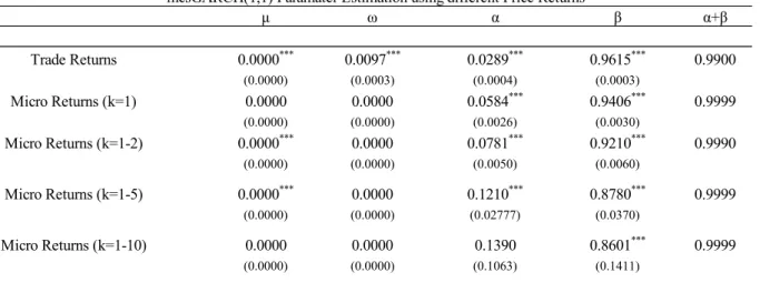
Table 1 summarises the estimated parameters from the (mcs)GARCH model (2.6). We find for all observed price returns that the conditional variance is highly persistent as the sum of α and β is close to 1. By construction, the parameters of the GARCH models are weights and thus we find the constant ω of the GARCH equation close to 0. Interestingly, with trade returns we find the constant of the variance equation (ω=0.0097) significant at the 1% nominal level with robust standard errors based on White’s correction (Ghalanos, 2018). For micro prices ‘ω’ is somewhat close to 0, but insignificant (none of the estimates is 0, but of the power of 1-e09). The same pattern holds for the constant μ of our mean equation, except for trade returns and micro returns (k=1-2), where we find a constant significantly different from 0. As imposed by the GARCH framework a constant of ω = 0 is undesirable, as it would suggest that mean-variance in the long-run is not existent. Bollerslev (1986) states the condition of 𝜔 > 0, without further explanation on model implication if this condition is violated. However, Nelson (1992) states that this condition can be less restricted and allows for 𝜔 ≥ 0 in the GARCH framework. If ω is 0 and the condition α + β = 1 is satisfied, then the GARCH(1,1) process becomes an Exponential Weighted Moving Average (EWMA). Thus, one can write α = 1- β and obtain the EWMA (J.P Morgan/Reuters, 1996), using formula (2.6)
𝜎-,.|.[KV = (1 − 𝛽)𝜀̅²
-,.[K+ 𝛽𝜎²-,.[K (4.0)
In this case the decay factor of the EWMA process is not arbitrarily chosen but estimated. The forecast of an EWMA, is a martingale, meaning that the best forecast for one-step ahead is the
For higher-level micro prices (k=1-10), we find that lagged innovations are found to be insignificant. This suggests a GARCH(0,q)-structure.
Table 1 – Coefficient estimation using 80% of the available sample
If the variance can be fully explained by an GARCH(0,1) process, we thus express the variance at time 𝑡, 𝑖 as
𝜎-,.² = 𝜔 + 𝛽𝜎
-,.[K² . (4.1)
From above’s equation one can use iterative substitution and show that, 𝜎² = r
K[s (4.2)
concluding that whatever value the initial conditional variance assumes, after a long enough time horizon the conditional variance will converge to a level around r
K[s implying
unconditional homoscedasticity. This means, it will collide with the law of motion implying that (4.1) holds. In a special case one can reconcile both if 𝜔=0 and 𝛽 = 1 for (4.1), where 𝜎-,.²
will be a constant and equal to the unconditional variance σ² (𝜎-,.² = σ²). Thus a
GARCH(0,q)-structure would be redundant. This is in line with Bollerslev’s (1986) stated condition, where p must be greater 0, whereas the q lag can be 0, implying an ARCH process.
μ ω α β α+β Trade Returns 0.0000*** 0.0097*** 0.0289*** 0.9615*** 0.9900 (0.0000) (0.0003) (0.0004) (0.0003) Micro Returns (k=1) 0.0000 0.0000 0.0584*** 0.9406*** 0.9999 (0.0000) (0.0000) (0.0026) (0.0030) Micro Returns (k=1-2) 0.0000*** 0.0000 0.0781*** 0.9210*** 0.9990 (0.0000) (0.0000) (0.0050) (0.0060) Micro Returns (k=1-5) 0.0000*** 0.0000 0.1210*** 0.8780*** 0.9999 (0.0000) (0.0000) (0.02777) (0.0370) Micro Returns (k=1-10) 0.0000 0.0000 0.1390 0.8601*** 0.9999 (0.0000) (0.0000) (0.1063) (0.1411) p-Value: *** Significance at 1%, ** Significane at 5%, * Significance at 10%, robust S.E. reported in brackets
Remarks: Reported Estimates in this table are not 0, but of the power of 1-e09.
We conclude, that micro prices, which are in our case the clearing price of the order book (Gatheral and Oomen, 2010) appear to have a long-run stable volatility and it seems like new innovations become more a white noise process the more levels are included. This may be intuitively due to the nature of the FESX market, where the vast majority of trades occur at the lower levels (recall stylized facts about FESX). This means that orders and corresponding sizes near the mid-price are more frequently updated and thus including higher levels is vanishing/averages out the effect of liquidity shocks at lower levels, as larger trades tend to be traded via TES.
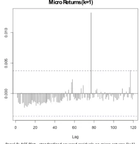
However, we find that micro returns tend to have better model specification properties, except for micro returns (k=1-2), when inspecting their residuals. Figure 4shows the ACF plots of the standardized squared residuals for the different input returns under the (mcs)GARCH. From visual inspection it clearly follows that the lagged residuals of the micro prices (Panel B, C and D) do not show any significant autocorrelation beside some random jumps, whereas standardized squared residuals in trade returns (Panel A) tend to be noisy. In fact, in panel C for standardized squared residuals on micro returns (k=1-2), we find a small but persistent negative memory effect. Moreover, including more levels, except for micro returns (k=2), results in more structured data as the jumps of the standardized squared residuals tend to decrease significantly. As the jumps for micro prices occur randomly, we assume that they do not harm the overall model quality. This pattern also holds for lags larger than 120 (2hrs), for example up to the 800th lag (1 trading day).
Figure 4 – ACF on standardized squared residuals
Micro Returns (k=1-5)
Panel D: ACF Plot - standardized squared residuals on micro returns (k=1-5)
Micro Returns (k=1-2)
Micro Returns (k=1-10)
Panel E: ACF Plot - standardized squared residuals on micro returns (k=1-10)
Trade Returns Micro Returns (k=1)
Panel A: ACF Plot - standardized squared residuals on trade returns Panel B: ACF Plot - standardized squared residuals on micro returns (k=1)
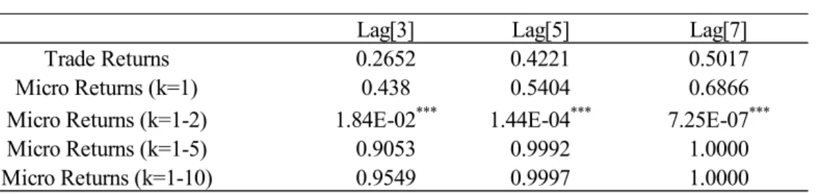
Furthermore, we find no ARCH effects prevailing for the standardized residuals, except for the micro returns (k=1-2). Table 2 summarises results of the ARCH LM test for different lags on the standardized residuals. As stated before, we used different lag specifications for each model, with special focus on micro returns (k=1-2). None of the tried combinations was able to capture the prevailing ARCH effects in the standardized residuals.
Table 2 – ARCH LM test based on 80% of the available sample for different returns
Appendix Figure 6shows the QQ-Plot on the residuals for the different returns. As one can see, the residuals of the micro prices follow the theoretical quantiles of the normal distribution closer compared to trade returns. This is especially true for quantiles in the centre of the distribution. For all return series the boundaries of the quantiles, the residuals heavily diverge from the normal. Even, when we assume the conditional distribution to be student’s t, the standardized residuals still tend to be heavily-tailed. This pattern manifests itself, the more order book levels are included and is mainly due to large outliers. As our sample size is rather large, testing for distribution under the null (e.g. Jarque-Bera, Wilkox-Shapiro or Kolmogorov-Smirnov) is difficult as these tests have large power (1- Prob(Error Type II)) and hence any small divergence from a distribution will be meaningful and will lead to reject the null.
Especially for trade returns one can find the drawbacks of microstructure properties in high-frequency data. As prices for the FESX occur on a relatively discrete level (1 index point), one can retrieve from the QQ-Plot Panel A that the frequency of 0% returns exceed those assumed by a normal distribution. This results in a horizontal line at the centre of the QQ-Plot.
Lag[3] Lag[5] Lag[7]
Trade Returns 0.2652 0.4221 0.5017
Micro Returns (k=1) 0.438 0.5404 0.6866
Micro Returns (k=1-2) 1.84E-02*** 1.44E-04*** 7.25E-07***
Micro Returns (k=1-5) 0.9053 0.9992 1.0000
Micro Returns (k=1-10) 0.9549 0.9997 1.0000
p-Value: *** Significance at 1%, ** Significane at 5%, * Significance at 10%
microstructure noise created by the bid-ask bounce.
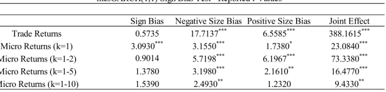
The proposed sign (size) bias test by Engle and Ng (1993) on residuals gives conclusion about the features that the model can capture. Using a de-seasonalized simple GARCH model, we assume shocks to be symmetric. Table 3 reports the sign bias test for different price returns.
Table 3 – Sign Bias Test based on 80% of the available sample for different returns
Trade returns fail to capture larger price swings in either direction as the size bias test is significant in both cases. This means the model overestimates smaller variations in returns and underestimates larger fluctuations in returns for volatility prediction. The sign bias is not significant, indicating that positive and negative shocks have the same influence, same holds for the micro returns (k=1-2). For micro returns it seems that the more levels are included the more of these features are jointly captured, as t-values are decreasing, but not for micro returns (k=1-2). Nevertheless, a simple GARCH model fails to estimate all variations in shocks properly with either price returns.
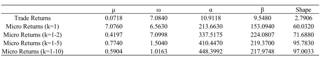
Additionally, we conclude that coefficient estimation in a high-frequency framework is highly time-varying as concluded by the Nyblom’s (1989) stability test summarized in Table 4. For most coefficients except for the mean-return μ, we find that the estimates are unstable over the estimation period. The more levels of the order book are included the more we find the coefficients to fluctuate.
Sign Bias Negative Size Bias Positive Size Bias Joint Effect
Trade Returns 0.5735 17.7137*** 6.5585*** 388.1615***
Micro Returns (k=1) 3.0930*** 3.1550*** 1.7380* 23.0840***
Micro Returns (k=1-2) 0.9014 5.7198*** 6.1967*** 73.3380***
Micro Returns (k=1-5) 1.3780 3.1980*** 2.1610** 16.4770***
Micro Returns (k=1-10) 1.5390 2.4930** 1.2320 9.4330**
p-Value: *** Significance at 1%, ** Significane at 5%, * Significance at 10%
Table 4 – Nyblom test statistics based on 80% of the available sample for different returns
In a high-frequency framework of 1-minute intervals over almost 1.5 years of data (80% of our total sample), we see that including more information about the state of the order book can lead to wrong statistical inference, when dealing with time-varying estimates. As stated earlier, the order book is updated in a frequently manner, and prevailing information about the state of the order book is not long-lasting. To have a better understanding about coefficient estimation in our data set, we try to capture structural breaks and time-varying market regimes by estimating a smaller sub-sample based on a rolling and a recursive window, where (1) shall show the time variation in the estimates along the sub-sample period and (2) to capture if there is an “optimal” estimation window-size where coefficients converge to a stable value.
The sub-sample was selected on a random basis and starts in September 14, 2017 and ends September 29, 2017, covering 10 full trading days. For the initial estimation window, we use 20% of the data (2 days) and proceed to re-estimate the coefficients every minute. As Appendix Figure 7 shows, all coefficients for micro returns are highly time-varying and indicate the prevalence of a daily pattern as they oscillate around every 800 observations (1 trading day). In contrast, the coefficients of trade returns are more stable, especially 𝜔. They fluctuate overtime, but the magnitude of fluctuation is relatively small compared to the fluctuations in the coefficients of micro returns.
Appendix Figure 8 shows the corresponding empirical distribution function of the coefficients. Due to the very small fluctuation of the trade returns’ coefficients, the distribution is very accumulated and has taken the shape of a vertical line. On the contrary, the distribution
μ ω α β Shape Trade Returns 0.0718 7.0840 10.9118 9.5480 2.7906 Micro Returns (k=1) 7.0760 6.5630 213.6630 153.0940 60.0320 Micro Returns (k=1-2) 0.4197 7.0998 337.5175 224.0807 71.6880 Micro Returns (k=1-5) 0.7740 1.5040 410.4470 219.3700 95.7830 Micro Returns (k=1-10) 0.5904 1.0163 448.3992 217.9748 97.0033
Critical Values for individual statistics: 0.75 (1%), 0.47 (5%), 0.35 (10%)
To show if the initial window size can affect the stability of the coefficient estimates, we run the same procedure but instead of a rolling window over time, we use an expanding window to estimate the coefficients. As before, the initial window will be 20% of our data set and will be successively expanded by 1-minute intervals. As can be observed in Appendix Figure 9, the majority of the coefficients do not stabilize as the window size increases. Only the coefficients of micro returns (k=1-10) appear to stabilize after 2,000 observations. The smallest time variation is to be found for trade returns, especially for α. Appendix Figure 10 shows the distribution of the estimated coefficients for the expanded window. Except for trade returns, the expanding window results in higher dispersed coefficient distributions.
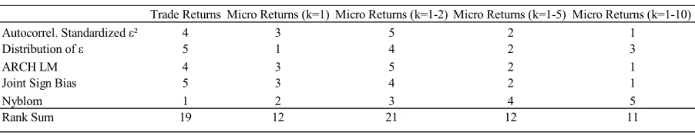
Table 5 reports the relative ranking of all tests conducted on the different return series. Micro returns (k=1-10) have the best features to capture model specification. It suffers least from autocorrelation in the squared standardized residuals, captures best the joint impact of asymmetric shocks, and has homoscedastic standardized residuals, indicated through the ARCH LM test. However, we find that coefficient estimates for higher-level return series suffer from estimation instability. Furthermore, the standardized residuals tend to be heavy tailed compared to a normal distribution. In the ranking micro returns (k=1-2) perform worst, where standardized squared residuals suffer from negative autocorrelation, and residuals still bear ARCH effects.
We do not claim that a good relative ranking induces that the model features were correctly specified (e.g. Joint Sign Bias Test) but indicates that it was performing better on a relatively basis. However, better estimation properties do not necessarily yield better forecasting abilities.
Table 5 – Relative ranking on model specification tests based on 80% of the available sample for different return series From visual inspection of Appendix Figure 11 we found that higher level micro returns share the same patterns as trade returns, while having better estimation features. To confirm this hypothesis, we conduct the Kolmogorov-Smirnov test on trade and micro returns (k=1-10) to check whether both return series are drawn from the same empirical distribution. Due to the large sample size we cannot perform the test on the whole sample at once (as explained before). To overcome this problem, we conduct the Kolmogorov-Smirnov test on a rolling window basis using different window sizes. Over the whole sample we count the estimated p-values that are larger than 5%. From Table 6 we conclude that the hypothesis that micro returns (k=1-10) and trade returns come from the same distribution must be rejected. As we increase the window size, we find that the minority of tested bins fall into the same empirical distribution. However, compared to lower-level micro returns, including more levels indicates weak evidence that they behave more like trade returns.
Table 6 – Kolmogorov-Smirnov test on trade returns and micro returns for different window sizes, where the window size equals the number of observations in each bin
Trade Returns Micro Returns (k=1) Micro Returns (k=1-2) Micro Returns (k=1-5) Micro Returns (k=1-10)
Autocorrel. Standardized ε² 4 3 5 2 1
Distribution of ε 5 1 4 2 3
ARCH LM 4 3 5 2 1
Joint Sign Bias 5 3 4 2 1
Nyblom 1 2 3 4 5
Rank Sum 19 12 21 12 11
Low rank indicates relative outperformance compared to other return series.
Remarks: Good ranking does not imply that criterion was necessarly statistically correctly specified
Estimation (Mis-)Specification Ranking using mcsGARCH(1,1)
30 60 90 120
Micro Returns (k=1) 77.82% 38.70% 11.31% 4.88%
Micro Returns (k=1-2) 78.08% 38.51% 11.39% 4.49%
Micro Returns (k=1-5) 79.51% 46.18% 16.38% 7.46%
Micro Returns (k=1-10) 78.92% 47.55% 18.37% 7.49%
Remarks: Percentage of observations where p-Value was greater than 5% significance
Rolling Window Kolmogorov-Smirnov Test Window Size
6. Conclusion
This research used 1-minute Euro Stoxx 50 Futures data under the multiplicative component GARCH framework to provide high frequency estimates on the volatility of different return series. The series consist of trade returns and micro price returns, of which the latter incorporate LOB information. This approach aims to overcome the problems of microstructure noise and intraday seasonality which are encountered when modelling volatility at such a high frequency. The model was applied to 423 trading days of which 80%, approximately 338 days, was used for estimation purposes.
Its findings reveal that properties of higher-level micro prices tend to have better model specifications, when focusing on standardized residuals. They suffer less from autocorrelation and follow more closely a normal distribution. However, we find that these higher-level micro prices are vulnerable to shocks in liquidity, as shown by the extreme outliers in the standardized residuals, and produce unstable coefficients. This instability is highly time-varying and very dependent on the window size. Based on the fixed windows estimation, micro return coefficients based on the GARCH(1,1) reveal that the volatility process follows more likely an Exponentially Weighted Moving Average, of which the decay factor is estimated.
To conclude, the more LOB information is incorporated the better the behaviour of the standardized residuals, since it follows to a greater extent a white noise process. This, however, at the cost of larger instability of the coefficients. These features are induced by the seasonality of liquidity and shocks in liquidity which are more severe for higher-level micro prices.
For further research one could examine the properties of micro prices of different asset classes and under different sampling frequencies. Additionally, further research could be conducted on the behaviour of the higher levels of the LOB and how this behaviour affects volatility. Moreover, it would be interesting to see if micro returns have superior properties for end of day realized volatility estimates and if indeed higher frequencies reveal the true nature of the volatility process during a trading day.
References
Anand, A., Chakravarty, S., & Martell, T. (2005). Empirical evidence on the evolution of liquidity: Choice of market versus limit orders by informed and uninformed traders.
Journal of Financial Markets, 289-309.
Andersen, T. G., & Bollerslev, T. (1998). Deutsche Mark-Dollar Volatility: Intraday Activity Patterns, Macroeconomic Announcements, and Longer Run Dependencies. The
Journal of Finance, Vol. 53.
Anderson, T. G., Bollerslev, T., Diebold, F. X., & Ebens, H. (2001). The distribution of realized stock return volatility. Journal of Financial Economics, 43-76.
Anderson, T., & Bollerslev, T. (1997). Intraday periodicity and volatility persistence in financial markets. Journal of Empirical Finance, Vol 4, 115-158.
Angel, J. J. (1997). Tick Size, Share Prices, and Stock Splits. The Journal of Finance, Vol.
52, 655-681.
Bollerslev, T. (1986). Generalized Autoregressive Conditional Heteroskedasticity. Jourlan of
Econometrics, Vol. 31, 302-327.
Bonart, J., & Lillo, F. (2016). A continuous and efficient fundamental price on the discrete order book grid. Working Paper - Cornell University.
Busch, T., Christensen, B. J., & Nielsen, M. O. (2011). The role of implied volatility in forecasting future realized volatility and jumps in foreign exchange, stock, and bond markets. Journal of Econometrics, Vol. 160, 48-57.
Cao, C., Hansch, O., & Wang Beardsley, X. (2004). The Informational Content of an Open Limit Order Book. Available at SSRN: https://ssrn.com/abstract=565324.
Cao, C., Hansch, O., & Wang, X. (2009). The information content of an open limit‐order book. Journal of Futures Markets, Vol. 29, 16-41.
Easley, D., López de Prado, M. M., & O'Hara, M. (2012). Flow Toxicity and Liquidity in a High-frequency World. The Review of Financial Studies, Vol. 25, 1457-1493. Engle, R. F., & Ng, V. K. (1993). Measuring and Testing the Impact of News on Volatility.
The Journal of Finance, Vol 48., 1749-78.
Engle, R. F., & Sokalska, M. F. (2012). Forecasting intraday volatility in the US equity market. Multiplicative component GARCH. Journal of Financial Econometrics, Vol.
10, 54-83.
Eurex Exchange - Matching Principles. (2018, November 30). Retrieved from Eurex
Exchange: http://www.eurexchange.com/exchange-en/trading/market-model/matching-principles
Eurex Exchange - Trading Statistics. (2018, November 30). Retrieved from Eurex Exchange:
European Securities and Markets Authority. (2014 (No. 1)). High-frequency trading activity
in EU equity markets. Paris: ESMA.
Fuest, A., & Mittnik, S. (2015). Modeling Liquidity Impact on Volatility: A GARCH-FunXL Approach. Working Paper Number 15, Center for Quantitative Risk Analysis.
Gatheral, J., & Oomen, R. C. (2010). Zero-Intelligence Realized Variance Estimation.
Finance and Stochastics, Vol.14, 249-283.
Ghalanos, A. (2018). Introduction to the rugarch package. . Available at:
https://cran.r-project.org/web/packages/rugarch/vignettes/Introduction_to_the_rugarch_package.p df.
Harris, L. (1998). Optimal dynamic order submission strategies in some stylized trading problems. Financial Markets, Institutions & Instruments 7, 1-76.
Hautsch, N., & Huang, R. (2011). The Market Impact of a Limit Order. Journal of Economic
Dynamics and Control.
J.P. Morgan; Reuters. (1996, December 17). MSCI. Retrieved from MSCI - Documents: https://www.msci.com/documents/10199/5915b101-4206-4ba0-aee2-3449d5c7e95a Jarnecic, E., & Snape, M. (2014). The Provision of Liquidity by High-Frequency
Participants. Financial Review, Vol. 49, 371-394.
Liu, L., Patton, A. J., & Sheppard, K. (2015). Does anything beat 5-Minute RV? A comparision of realized measures across multiple asset classes. The Journal of
Econometrics, 293-311.
Malec, P. (2016). A Semiparametric Intraday GARCH Model. Available at SSRN:
https://ssrn.com/abstract=2785615.
Neetson, D. (2018, December 6). LinkedIn Conversation: Model complexity and latency problems in high-freuqency trading. (M. Grübe, Interviewer)
Nelson, D. B. (1992). Inequality Constraints in the Univariate GARCH Model. Journal of
Business & Economic Statistics, Vol. 10, 229-35.
Nyblom, J. (1989). Testing for the Constancy of Parameters over Time. Journal of the
American Statistical Association, Vol. 84, 223-230.
Rock, K. (1996). The specialist's order book and price anomalies. Working Paper.
Stoikov, S. (2017). The Micro-Price: A High Frequency Estimator of Future Prices. Available
at SSRN: https://ssrn.com/abstract=2970694 or http://dx.doi.org/10.2139/ssrn.2970694.
Zhang, L., Mykland, P. A., & Ait-Sahalia, Y. (2005). A Tale of Two Time Scales:
Determining Integrated Volatility With Noisy High-Frequency Data. Journal of the
Appendix
Appendix Figure 1 – Seasonality pattern in order book depth and trade activity. Shown is the median depth and median cumulative number of trades for each 1-minute interval over the sample period.
Appendix Figure 2 – QQ-Plot for different returns
Trade Returns Micro Returns (k=1)
Micro Returns (k=1-5)
Micro Returns (k=1-10)
Panel A: QQ Plot on trade returns Panel B: QQ Plot on micro returns (k=1)
Panel D: QQ Plot on micro returns (k=1-5)
Panel E: QQ Plot on micro returns (k=1-10) Panel C: QQ Plot on micro returns (k=1-2)
Micro Returns (k=1-5)
Panel D: ACF Plot - micro returns (k=1-5)
Micro Returns (k=1-2)
Micro Returns (k=1-10)
Panel E: ACF Plot - micro returns (k=1-10)
Trade Returns
Panel A: ACF Plot - trade returns Panel B: ACF Plot - micro returns (k=1)
Panel C: ACF Plot - micro returns (k=1-2)
Appendix Figure 4 – Different price series for 2.5 hours of data
Trade Returns Micro Returns (k=1)
Micro Returns (k=1-5)
Micro Returns (k=1-10)
Panel A: QQ Plot on standardized residuals Panel B: QQ Plot on standardized residuals
Panel D: QQ on standardized residuals
Panel E: QQ Plot on standardized residuals Panel C: QQ on standardized residuals
Appendix Table 1 – Descriptive trade and LOB statistics based on 1-minute intervals. Trade activity is based on the number of occurred trades within an interval, mean volume is based on the mean traded volume within a minute, sell-ratio is based on the number of trades that were initiated by a sell order divided by the total number of trades (trade activity) that occurred within the 1-minute interval, spread is defined as the difference between best ask and best bid price and depth is defined as the cumulative volume of all order book levels (bid and ask).
Trade Activity Mean Volume Sell Ratio Spread Depth
Min 1 1 0 -35 472 1st Quartile 12 8.9 0.3333 1 12503 Median 28 16.92 0.5 1 16429 3rd Quartile 56 27.05 0.6562 1 19468 Max 1837 772 1 3 56626 Mean 43.32 20.46 0.4952 0.9223 16335