Measurements of differential production cross sections for a Z boson in association with jets in pp collisions at $ \sqrt{s}=8 $ TeV

(1)

CERN-EP/2016-256 2017/05/25

CMS-SMP-14-013

Measurements of differential production cross sections for

a Z boson in association with jets in pp collisions at

_√

s

=

8 TeV

The CMS Collaboration

∗

Abstract

Cross sections for the production of a Z boson in association with jets in proton-proton

collisions at a centre-of-mass energy of√s=8 TeV are measured using a data sample

collected by the CMS experiment at the LHC corresponding to 19.6 fb−1. Differential

cross sections are presented as functions of up to three observables that describe the jet kinematics and the jet activity. Correlations between the azimuthal directions and the rapidities of the jets and the Z boson are studied in detail. The predictions of a number of multileg generators with leading or next-to-leading order accuracy are compared with the measurements. The comparison shows the importance of including multi-parton contributions in the matrix elements and the improvement in the predictions when next-to-leading order terms are included.

Published in the Journal of High Energy Physics as doi:10.1007/JHEP04(2017)022.

c

2017 CERN for the benefit of the CMS Collaboration. CC-BY-3.0 license

∗_{See Appendix A for the list of collaboration members}

(2)

(3)

1 Introduction

The high centre-of-mass energy of proton-proton (pp) collisions at the CERN LHC produces

events with large jet transverse momenta (pT) and high jet multiplicities in association with a

Z/γ∗ boson. For convenience Z/γ∗ is denoted as Z. The selection of events in which the Z

boson decays into two oppositely charged electrons or muons provides a signal sample that is not significantly contaminated by background processes. This decay channel can be recon-structed with high efficiency due to the presence of charged leptons in the final state and is well suited for the validation of calculations within the framework of perturbative quantum chromodynamics (QCD). Furthermore, the production of massive vector bosons with jets is an important background to a number of standard model (SM) processes (single top and tt pro-duction, vector boson fusion, WW scattering, Higgs boson production) as well as searches for physics beyond the SM. A good understanding of this background is vital to these searches and measurements. Perturbative QCD calculations of the differential cross sections involve

differ-ent powers of the strong coupling constant αsand different kinematic scales and are therefore

technically challenging. The issue has been addressed over the last 15 years by merging pro-cesses with different parton multiplicities before the parton showering, initially at tree level, and more recently with matrix elements calculated at next-to-leading order (NLO) using mul-tileg matrix-element (ME) event generators [1, 2].

In this paper we present measurements of the differential cross sections for Z boson

produc-tion in associaproduc-tion with jets at√s = 8 TeV, in the electron and muon decay channels, using

a data sample corresponding to an integrated luminosity of 19.6 fb−1. Our measurements are

compared with calculations obtained from different multileg ME event generators with leading order (LO) MEs (tree level), NLO MEs and a combination of NLO and LO MEs. Measurements

of the Z+jets cross section were previously reported by the CDF and D0 Collaborations in

proton-antiproton (pp) collisions at a centre-of-mass energy√s = 1.96 TeV [3, 4]. More recent

results from proton-proton (pp) collisions at√s = 7 TeV were published by the ATLAS [5, 6]

and CMS [7, 8] Collaborations.

The cross sections are restricted to the phase space where the lepton transverse momenta are greater than 20 GeV, their absolute pseudorapidities are less than 2.4, and the dilepton mass is

in the interval 91±20 GeV. The jets are defined using the infrared and collinear safe anti-kt

al-gorithm applied to all visible particles; the radius parameter is set to 0.5 [9]. The four-momenta of the particles are summed and therefore the jets can be massive. The differential cross sec-tions include only those jets with transverse momentum greater than 30 GeV and further than

R = 0.5 from the leptons in the (η, φ)-plane, where φ is the azimuthal angle. In addition, the

absolute jet rapidity is required to be smaller than 2.4. The jets are referred to as 1st, 2nd, 3rd,

etc. according to their transverse momenta, starting with the highest-pT jet, and denoted as j1,

j₂, j₃, etc. To further investigate the QCD dynamics towards low Bjorken-x values,

multidimen-sional differential cross sections are measured for Z+ ≥1 jet production in an extended phase

space with jet rapidities up to 4.7. The extension of the rapidity coverage from 2.4 to 4.7 is used

to tag events from vector boson fusion (e.g., Higgs production). Typically, the Z+jets events

constitute a background for such processes, and a good understanding of their production dif-ferential cross section including jets in the forward region is important.

For each jet multiplicity (Njets) a number of measurements are made: the total cross section in

the defined phase space, the differential cross sections as functions of the jet transverse

mo-mentum scalar sum HT, and the differential cross sections as a function of the individual jet

kinematics (transverse momentum pT, and absolute rapidity|y|). For the leading jet a double

(4)

mo-mentum. Correlations in the jet kinematics are studied with one-dimensional and multidimen-sional differential cross section measurements, via 1) the distributions in the azimuthal angles between the Z boson and the leading jet and between the two leading jets, and 2) the rapidity distributions of the Z boson and the leading jet. These two rapidities are used as variables of a three-dimensional differential cross section measurement together with the transverse momen-tum of the jet. The Lorentz boost along the beam axis introduces a large correlation amongst the Z boson and the jet rapidities. The two rapidities are combined to form a variable

un-correlated with the event boost along the beam axis, ydiff = 0.5|y(Z) −y(ji)| and a highly

boost-dependent variable, ysum = 0.5|y(Z) +y(ji)|. The cross section is measured separately

as a function of each of these variables. The distribution of ydiffis mostly sensitive to the parton

scattering, while ysumis expected to be sensitive to the parton distribution functions (PDFs) of

the proton.

The Drell–Yan process, where the Z boson can decay into a pair of neutrinos, is a background to searches for new phenomena, such as dark matter, supersymmetry and other theories beyond the SM that predict the presence of invisible particle(s) in the final state. It is particularly impor-tant when the Z boson has a large transverse momentum, leading to a large missing transverse energy. The azimuthal angle between the jets is a good handle to suppress backgrounds

com-ing from QCD multijet events, while the HT variable can be used to select events with large

jet activity. For such analyses it is important to have a good model of Z+jets production and

therefore a good understanding of these observables. This motivates the measurement of the distributions of the azimuthal angles between the jets and between the Z boson and the jets for

different thresholds applied to the Z boson transverse momentum, the HTvariable, and the jet

multiplicity. These angles can be measured with high precision, and thus provide an excellent avenue to test the accuracy of SM predictions [10]. The dijet mass is an essential observable in the selection of Higgs boson events produced by vector boson fusion and it is important

to model well both this process and its backgrounds. This observable is measured in Z+jets

events for the two leading jets.

Section 2 describes the experimental setup and the data samples used for the measurements, while the object reconstruction and the event selection are presented in Section 3. Section 4 is dedicated to the subtraction of the background contribution and the correction of the detector response, and Section 5 to the estimation of the measurement uncertainties. Finally, the results are presented and compared to different theoretical predictions in Section 6 and summarised in Section 7.

2 The CMS detector, simulation, and data samples

The central feature of the CMS apparatus is a superconducting solenoid of 6 m internal diame-ter, providing a magnetic field of 3.8 T. Within the solenoid volume are a silicon pixel and strip

tracker covering the range|η| <2.5 together with a calorimeter covering the range|η| <3. The

latter consists of a lead tungstate crystal electromagnetic calorimeter (ECAL), and a brass and scintillator hadron calorimeter (HCAL). The HCAL is complemented by an outer calorimeter placed outside the solenoid used to measure the tails of hadron showers. The pseudorapidity

coverage is extended up to|η| = 5.2 by a forward hadron calorimeter built using

radiation-hard technology. Gas-ionization detectors exploiting three technologies, drift tubes, cathode strip chambers, and resistive-plate chambers, are embedded in the steel flux-return yoke out-side the solenoid and constitute the muon system, used to identify and reconstruct muons over

the range|η| <2.4. A more detailed description of the CMS detector, together with a definition

(5)

Simulated events are used to both subtract the contribution from background processes and to correct for the detector response. The signal and the background (from WW, WZ, ZZ, tt, and single top quark processes) are modelled with the tree-level matrix element event generator

MADGRAPHv5.1.3.30 [12] interfaced withPYTHIA6.4.26 [13]. The PDF CTEQ6L1 [14] and the

Z2* PYTHIA6 tune [15, 16] are used. For the ME calculations, αsis set to 0.130 at the Z boson

mass scale. The five processes pp → Z + Njets jets, Njets = 0, . . . , 4, are included in the ME

calculations. The kt−MLM [17, 18] scheme with the merging scale set to 20 GeV is used for

the matching of the parton showering (PS) with the ME calculations. The same setup is used

to estimate the background from Z+jets → τ+τ−+ jets. The signal sample is normalised

to the inclusive cross section calculated at next-to-next-to-leading order (NNLO) with FEWZ

2.0 [19] using the CTEQ6M PDF set [14]. Samples of WW, WZ, ZZ events are normalised to the

inclusive cross section calculated at NLO using theMCFM6.6 [20] generator. Finally, an NNLO

plus next-to-next-to-leading log (NNLO + NNLL) calculation [21] is used for the normalisation of the tt sample. When comparing the measurements with the predictions from theory, several other event generators are used for the Drell–Yan process. Those, which are not used for the measurement itself, are described in Section 6.

The detector response is simulated with GEANT4 [22]. The events reconstructed by the

detec-tor contain several superimposed proton-proton interactions, including one interaction with a

high pT track that passes the trigger requirements. The majority of interactions, which do not

pass trigger requirements, typically produce low energy (soft) particles because of the larger cross section for these soft events. The effect of this superposition of interactions is denoted as pileup. The samples of simulated events are generated with a distribution of the number of proton-proton interactions per beam bunch crossing close to the one observed in data. The number of pileup interactions, averaging around 20, varies with the beam conditions. The correct description of pileup is ensured by reweighting the simulated sample to match the measured distribution of pileup interactions.

3 Event reconstruction and selection

Events with at least two leptons (electrons or muons) are selected. The trigger accepts events

with two isolated electrons (muons) with a pT of at least 8 and 17 GeV. After reconstruction

these leptons are restricted to a kinematic and geometric acceptance of pT > 20 GeV and|η| <

2.4. We require that the oppositely charged, same-flavor leptons form a pair with an invariant

mass within a window of 91±20 GeV. The ECAL barrel-endcap transition region 1.444< |η| <

1.566 is excluded for the electrons. The acceptance is extended to the full|η| <2.4 region when

correcting for the detector response.

Information from all detectors is combined using the particle-flow (PF) algorithm [23, 24] to produce an event consisting of reconstructed particle candidates. The PF candidates are then used to build jets and calculate lepton isolation. The quadratic sum of transverse momenta of the tracks associated to the reconstructed vertices is used to select the primary vertex (PV) of interest. Because pileup involves typically soft particles, the PV with the highest sum is chosen. The electrons are reconstructed with the algorithm described in Ref. [25]. Identification criteria based on the electromagnetic shower shape and the energy sharing between ECAL and HCAL are applied. The momentum is estimated by combining the energy measurement in the ECAL with the momentum measurement in the tracker. For each electron candidate, an isolation variable, quantifying the energy flow in the vicinity of its trajectory, is built by summing the

transverse momenta of the PF candidates within a cone of size∆R =

√

(6)

excluding the electron itself and the charged particles not compatible with the primary event vertex. This sum is affected by neutral particles from pileup events, which cannot be rejected

with a vertex criterion. An average energy density per unit of∆R is calculated event by event

using the method introduced in Ref. [26] and used to estimate and subtract the neutral particle contribution. The electron is considered isolated if the isolation variable value is less than 15% of the transverse momentum of the electron. The electron candidates are required to be consistent with a particle originating from the PV in the event.

Muon candidates are matched to tracks measured in the tracker, and they are required to sat-isfy the identification and quality criteria described in Ref. [27] that are based on the number of tracker hits and the response of the muon detectors. The background from cosmic ray muons, which appear as two back-to-back muons, is reduced by criteria on the impact parameter and by requiring that the muon pairs have an acollinearity larger than 2.5 mrad. An isolation

vari-able is defined that is similar to that for electrons, but with a cone size∆R=0.4 and a different

approach to the subtraction of the contribution from neutral pileup particles. For the muons this contribution is estimated from the sum of the transverse momenta of the charged particles rejected by the vertex requirement, considered as coming from pileup. This sum is multiplied by a factor of 0.5 to take into account the relative fraction of neutral and charged particles. A muon is considered isolated if the isolation variable value is below 20% of its transverse mo-mentum.

The efficiencies for the lepton trigger, reconstruction, and identification are measured with the “tag-and-probe” method [28]. The simulation is corrected using the ratios of the efficiencies obtained in the data sample to those obtained in the simulated sample. These scale factors for lepton reconstruction and identification typically range from 0.95 to 1.05 depending on the lepton transverse momentum and rapidity. The overall efficiency of trigger and event selection is 58% for the electron channel and 88% for the muon channel.

The anti-kT algorithm, with a radius parameter of 0.5, is used to cluster PF candidates to form

hadronic jets. The jet momentum is determined as the vectorial sum of all particle momenta. Charged hadrons identified as coming from a pileup event vertex are rejected from the jet clus-tering. The remaining contribution from pileup events, which comes from neutral hadrons and from charged hadrons whose PV has not been unambiguously identified, is estimated and subtracted event-by-event using a technique based on the jet area method [9, 29]. Jet energy corrections are derived from the simulation, and are confirmed with in situ measurements us-ing the energy balance of dijet and photon+jet events [30]. Jets with a transverse momentum

less than 30 GeV or overlapping within∆R = 0.5 with either of the two leptons from the

de-cay of the Z boson are discarded. The single differential cross sections are measured for jet

rapidity within|y| < 2.4, which is the region with the best jet resolution and pileup rejection.

In this measurement, the jet multiplicity refers to the number of jets fulfilling the jet criteria,

within the|y| <2.4 boundary for the one-dimensional differential cross sections. For the

mul-tidimensional differential cross sections reported in Section 6.8 the region for the jet rapidity is

extended to|y| <4.7.

4 Background subtraction and correction for the detector response

In Fig. 1 the event yield in the electron and muon channels is compared to the simulation.

The agreement between simulation and data is excellent up to four jets. Since the Z+jets

simulation does not include more than four partons in the ME calculations, we expect a less accurate prediction of the signal for jet multiplicities above four. Background contamination is below 1% for a jet multiplicity of one and increases with the jet multiplicity. The background

(7)

represents 2% of the event yield for a jet multiplicity of 2 and 20% for a jet multiplicity of 5. = 0 = 1 = 2 = 3 = 4 = 5 = 6 = 7 # Events 10 2 10 3 10 4 10 5 10 6 10 7 10 8 10 ee data and W τ τ → * γ Z/ and single t t t WW, WZ, ZZ ee → * γ Z/ CMS (8 TeV) -1 19.6 fb jets N = 0 = 1 = 2 = 3 = 4 = 5 = 6 = 7 Simulation/Data 0.6 0.8 1 1.2 1.4 = 0 = 1 = 2 = 3 = 4 = 5 = 6 = 7 # Events 10 2 10 3 10 4 10 5 10 6 10 7 10 8 10 9 10 data µ µ and W τ τ → * γ Z/ and single t t t WW, WZ, ZZ µ µ → * γ Z/ CMS (8 TeV) -1 19.6 fb jets N = 0 = 1 = 2 = 3 = 4 = 5 = 6 = 7 Simulation/Data 0.6 0.8 1 1.2 1.4

Figure 1: Exclusive jet multiplicity for (left) the electron and (right) the muon channels at

de-tector level in the jet rapidity region|y| <2.4. The data points are shown with statistical error

bars. Beneath each plot the ratio of the number of events predicted by the simulation to the measured values is displayed, together with the statistical uncertainties in simulation and data added in quadrature.

The background contribution is estimated from the samples of simulated events described in

Section 2 and subtracted bin-by-bin from the data. The simulations are validated using a µ±e∓

data control sample, as explained in Section 5. The background contribution from multijet events where the jets are misidentified as leptons is checked with a lepton control sample using two leptons with the same flavor and charge and found to be negligible.

Unfolding the detector response corrects the signal distribution for the migration of events be-tween closely separated bins and across boundaries of the fiducial region. The unfolding pro-cedure also includes a correction for the efficiency of the trigger, and the lepton reconstruction and identification. The unfolding procedure is applied separately to each measured differential cross section. In a first step, the data distribution is corrected to remove the background con-tribution and the concon-tribution from signal process events outside of the defined phase space. Then, the iterative D’Agostini method [31], as implemented in the statistical analysis toolkit

ROOUNFOLD[32], is used to correct for bin-to-bin migration and for efficiency. Using the

sim-ulation the method generates a response matrix that relates the probability that an event in bin i of the differential cross section is reconstructed in bin j. These probabilities include the case of bin-i events that do not pass the selection criteria on the reconstructed event or fall outside the distribution boundaries. For the three-dimensional differential cross section, the

method is applied within each(y(j₁), y(Z))bin, where the unfolding is performed with respect

to the pT(j1)observable. Similarly, the unfolding of the double differential cross sections is

per-formed with respect to the most sensitive variable: pT(j1)for d2σ/dpT(j1)dy(j1)and y(j1)for

(8)

The response matrices are built from reconstructed and generated quantities using the MAD

-GRAPH 5 + PYTHIA 6 Z+jets simulation sample. The generated values refer to the leptons

from the decay of the Z boson and to the jets built from the stable particles using the same

algorithm as for the measurements. The momenta of all the photons whose∆R distance to the

lepton axis is smaller than 0.1 are added to the lepton momentum to account for the effects of final-state radiation, and the lepton is said to be “dressed”. Although this process does not recover all the final-state radiation; it removes most differences between electrons and muons, and the dilepton mass spectra are identical for the two decay channels after this procedure, as

checked with the MADGRAPH5 +PYTHIA6 simulation. The Z boson is reconstructed from the

dressed lepton momentum vectors.

The phase space for the cross section measurement is restricted to pT > 20 GeV and|η| < 2.4

for both dressed charged leptons, a dilepton mass within 91±20 GeV, and the jet kinematics

constrained to pT > 30 GeV and|y| < 2.4. For the extended multidimensional cross sections

the phase space is extended to |y| < 4.7. The measured cross section values include the Z

branching fraction to a single lepton flavour.

The rejection of jets originating from pileup is more difficult outside the tracker geometric acceptance, since the vertex constraint cannot be used to reject the charged particles coming from pileup. Consequently, despite the jet pileup rejection criterion, a contamination of jets from pileup remains and needs to be subtracted. This region beyond the tracker acceptance,

2.5 < |y| < 4.7, is used only for the Z+ ≥ 1 jet multidimensional differential cross section

measurements, where only the leading jet is relevant. The fraction of events in which a jet

comes from pileup, denoted as fPU, is estimated using a control sample of a Z boson associated

with one jet, obtained by requiring one jet with pT above 30 GeV and a veto condition of no

other jets with pT > 12 GeV and above 20% of the Z boson transverse momentum. Since a Z

boson and a jet coming from two different pp collisions are independent, the distribution of

∆φ(Z, j)is expected to be flat, which is confirmed by the simulation. For the Z boson and the jet

from a pp→ Z+1 jet event the distribution is expected to peak at π. The constraint on

addi-tional jets enforces the pTbalance between the Z boson and the jet, reducing the contribution to

low values of∆φ(Z, j). The simulation shows that this contribution is negligible in the region

∆φ(Z, j) <1. Therefore, fPUis estimated from the fraction of events in that region. The value of

fPUis 30% in the most forward part (3.2< |y| <4.7) and lowest pTmeasurement bin (30 GeV

to 40 GeV). The fraction of pileup events estimated from the pileup control sample is used to correct the signal data sample. The same method is applied to the simulation. The ratio of the

value of fPUobtained from the simulation to that measured in data decreases monotonically as

a function of pT. In the pTbin 30–50 GeV it ranges up to 1.25 (1.35) for|y(j1)|between 2.5 and

3.2 (3.2 and 4.7). Beyond pT =50 GeV the discrepancy is negligible and the results are identical

with or without the pileup subtraction.

Since the |y(j)| < 2.4 region contains the bulk of the events and including the |y(j)| > 2.4

region does not improve the precision of the measurement, most of the differential cross section

measurements are limited to|y(j)| <2.4. The subtraction of pileup contributions is not needed

when confining measurements to this region.

5 Systematic uncertainties

The systematic uncertainty in the background-subtracted data distributions is estimated by varying independently each of the contributing factors before the unfolding, and computing the difference induced by the variation in the unfolded distributions. The observed difference between the positive and negative uncertainties is small and the two are therefore averaged.

(9)

The different sources of uncertainties are independent and are added in quadrature. The un-folded histogram can be written as a linear combination of the bin contents of the background-subtracted data histogram [31]. This linear combination is used to propagate analytically the statistical uncertainties to the unfolded results and calculate the full covariance matrix for each distribution, separately for each Z boson decay channel. The dominant source of systematic uncertainties is the jet energy correction. The various contributions are listed in Table 1. The jet energy correction uncertainty (JEC in the table) is calculated by varying this correction

by one standard deviation. This uncertainty is pT- and η-dependent and varies from 1.5% up

to 5% for|η| < 2.5 and from 7% to 30% for|η| > 2.5. The uncertainty in the measured cross

section is between 5.3% and 28% depending on the jet multiplicity. The jet energy resolution (JER) uncertainty is estimated for data and simulation in Ref. [33]. The resulting uncertainty in the measurement is below 1% for all the multiplicities.

Table 1: Cross section results obtained from the combination of the muon and electron channels as a function of the exclusive jet multiplicity and details of the systematic uncertainties. The column denoted Tot unc contains the total uncertainty; the column denoted Stat contains the statistical uncertainty; the remaining columns contain the systematic uncertainties.

Njets _dNdσ_jets Tot unc Stat JEC JER Bkg PU Unf stat Unf sys Lumi Eff

[pb] [%] [%] [%] [%] [%] [%] [%] [%] [%] [%] =0 423 3.7 0.034 1.2 0.06 0.002 0.71 0.05 1.2 2.6 1.8 =1 59.9 6.3 0.11 5.3 0.23 0.042 0.26 0.075 1.4 2.6 1.8 =2 12.6 9.2 0.25 8.4 0.22 0.33 0.35 0.12 1.7 2.7 1.9 =3 2.46 12 0.6 11 0.22 0.76 0.42 0.22 2.7 2.9 2.0 =4 0.471 16 1.4 15 0.16 1.3 0.57 0.43 3.5 3.1 2.1 =₅ _0.0901 ₂₀ _3.4 ₁₉ _0.28 _1.9 _0.75 _1.0 _4.6 _3.2 _2.3 =6 0.0143 33 9.3 28 0.72 3.3 1.9 2.4 5.5 3.7 2.6 =7 0.00230 34 22 23 0.61 4.3 5.6 6.3 6.4 3.9 2.8

Other significant background contributions come from tt, diboson, and Z → τ+τ− processes.

The related uncertainty (Bkg) is estimated by varying the cross section for each of the back-ground processes (tt, ZZ, WZ, and WW) independently by 10% for tt and 6% for diboson pro-cesses. The normalisation variation for the tt events is chosen to cover the maximum observed difference between the simulation and the data in the jet multiplicity, transverse momentum, and rapidity distributions when selecting events with two leptons of oppositely charged,

dif-ferent flavours (µ±e∓). The uncertainty in diboson cross sections covers theoretical and PDF

contributions. The resulting uncertainty in the measurement increases with the jet multiplicity and reaches 4.3%.

Another source of uncertainty is the modelling of the pileup (PU). The number of interactions per bunch crossing in simulated samples is varied by 5%. This covers effects related to the modeling of simulated minimum bias events of 3%, the estimate of the number of interactions per bunch crossing in data based on luminosity measurements of 2.6%, and the experimental uncertainties entering inelastic cross section measurements of 2.9%. The resulting uncertainties range from 0.26% to 5.6% depending on the jet multiplicity. The uncertainty from the pileup

subtraction performed in the forward region,|y| > 2.5, is estimated by varying up and down

the pileup fraction fPU described in Section 4 by half the difference from the value obtained

in the simulation. In the region covered by the tracker and where no correction is applied, it is verified that the jet multiplicity does not depend on the number of vertices reconstructed in the event. This indicates that the jets from pileup events have a negligible impact on the measurement.

(10)

The unfolding procedure has an uncertainty due to its dependence on the simulation used to estimate the response matrix (Unf sys) and to the finite size of the simulation sample (Unf stat).

The first contribution is estimated using an alternative event generator, SHERPA 1.4 [34], and

taking the difference between the two results to represent the uncertainty. The distribution obtained with the alternative generator differs sufficiently from the nominal one to cover the differences with the data. The statistical uncertainty in the response matrix is analytically prop-agated to the unfolded result [31]. When added in quadrature and depending on the kinematic variable and jet multiplicity, the total unfolding uncertainty varies up to 10%.

The uncertainty in the efficiency of the lepton reconstruction, identification, and isolation is propagated to the measurement by varying the total data-to-simulation scale factor by one standard deviation. It amounts to 2.5% and 2.6% in the dimuon and dielectron channels, re-spectively.

The uncertainty in the integrated luminosity amounts to 2.6% [35]. Since the background event yield normalisation also depends on the integrated luminosity, the effect of the above uncer-tainty on the background yield (Lumi) can be larger and amounts to 3.9% in the bins with low signal purity.

6 Results

The measurements from the electron and muon channels are consistent and are combined us-ing a weighted average. For each bin of the measured differential cross sections, the results of each of the two measurements are weighted by the inverse of the squared total uncertainty. The covariance matrix of the combination, the diagonal elements of which are used to extract the measurement uncertainties, is computed assuming full correlation between the two chan-nels for all the uncertainty sources except for statistical uncertainties and those associated with lepton reconstruction and identification, which are taken to be uncorrelated. The measured differential cross sections are compared to the results obtained from three different calculations as described below.

6.1 Theoretical predictions

The measurements are compared to a tree level calculation and two multileg NLO calculations.

The first prediction is computed with MADGRAPH5 [12] interfaced withPYTHIA6 (denoted as

MG5 + PY6 in the figure legends), for parton showering and hadronisation, with the configu-ration described in Section 2. The total cross section is normalised to the NNLO cross section

computed withFEWZ2.0 [19]. Two multileg NLO predictions including parton showers using

the MC@NLO [36] method are used. For these two predictions the total cross section is nor-malised to the one obtained with the respective event generators. The total cross section values used for the normalisation are summarised in Table 2.

The first multileg NLO prediction with parton shower is computed withSHERPA2 (2.0.0) [34]

and BLACKHAT [37, 38] for the one-loop corrections. The matrix elements include the five

processes pp → Z+Njets jets, Njets ≤ 4, with an NLO accuracy for Njets ≤ 2 and LO accuracy

for Njets = 3 or 4. The CT10 PDF [39] is used for both the ME calculations and showering

description. The merging of PS and ME calculations is done with the MEPS@NLO method [1] and the merging scale is set to 20 GeV.

The second multileg NLO prediction is computed with MadGraph5 aMC@NLO [40] (denoted

as MG5 aMC in the following) interfaced with PYTHIA 8 using the CUETP8M1 tune [16, 41]

(11)

Table 2: Values of the pp → `+_`−_{total inclusive cross section used in the predictions in} data-theory comparison plots. The cross section used for the plots together with the one obtained from the generated sample (“native”) and their ratio (k) are provided. The cross section values correspond to the dilepton mass windows used for the respective samples and indicated in the table.

Dilepton mass Native cross Used cross

Prediction window [GeV] section [pb] Calculation section [pb] k

MADGRAPH5 +PYTHIA6,≤4 j LO+PS >50 983 FEWZ NNLO 1177 1.197

SHERPA2,≤2 j NLO, 3, 4 j LO+PS [66, 116] 1059 native 1059 1

MG5 aMC+PYTHIA8,≤2 j NLO >50 1160 native 1160 1

the Z boson production processes with 0, 1, and 2 partons at NLO. The FxFx [2] merging scheme is used with a merging scale parameter set to 30 GeV. The NNPDF 3.0 NLO PDF [42] is used for the ME calculations while the NNPDF 2.3 QCD + QED LO [43, 44] is used for

the backward evolution of the showering. For the ME calculations, αs is set to the current

PDG world average [45] rounded to αs(mZ) = 0.118. For the showering and underlying

events the value of the CUETP8M1 tune, αs(mZ) = 0.130, is used. The larger value is

ex-pected to compensate for the missing higher order corrections. NLO accuracy is achieved for

pp→Z+Njets jets, Njets =0, 1, 2 and LO accuracy for Njets =3. For this prediction, theoretical

uncertainties are computed and include the contribution from the fixed-order calculation and from the NNPDF 3.0 PDF set. The two uncertainties are added in quadrature. The fixed-order calculation uncertainties are estimated by varying the renormalisation and the factorisation scales by factors of 1/2 and 2. The envelope of the variations of all factor combinations, ex-cluding the two combinations when one scale is varied by a factor 1/2 and the other by a factor

2, is taken as the uncertainty. The reweighting method [46] provided by the MG5 aMC

gen-erator is used to derive the cross sections with the different renormalisation and factorisation scales and with the different PDF replicas used in the PDF uncertainty determination. For the

NLO predictions, weighted samples are used (limited to±1 weights in the case of aMC@NLO),

which can lead to larger statistical fluctuations than expected for unweighted samples in some bins of the histograms presented in this section.

6.2 Jet multiplicity

The cross sections for jet multiplicities from 0 to 7, and the comparisons with various predic-tions are presented in this section. Figure 2 shows the cross section for both inclusive and exclusive jet multiplicities and the numbers are compared with the prediction obtained with

MG5 aMC +PYTHIA 8 in Table 3 for the exclusive case. The agreement with the predictions is

very good for jet multiplicities up to the maximum number of final-state partons included in

the ME calculations, namely three forMG5 aMC+PYTHIA8 and four for both MADGRAPH5 +

PYTHIA6 andSHERPA2. The level of precision of the measurement does not allow us to probe

the improvement expected from the additional NLO terms. The cross section is reduced by a factor of five for each additional jet.

The predictions already agree well at tree level (MADGRAPH 5 +PYTHIA 6) renormalised to

the NNLO inclusive cross section. For Njets = 4, theMG5 aMC+PYTHIA 8 calculation, which

does not include this jet multiplicity in the matrix elements, predicts a different cross section from those that do. The predictions that include four jets in the matrix elements are in better agreement with the data, but the difference between the predictions is limited to roughly one standard deviation of the measurement uncertainty. The large uncertainty is due to the

sen-sitivity of the jet pT threshold acceptance to the jet energy scale. TheSHERPA 2 prediction for

(12)

in-cludes this multiplicity in the ME calculations. The theoretical uncertainty shown in the figure

for theMG5 aMC +PYTHIA 8 prediction uses the standard method described in the previous

subsection. In the case of the exclusive jet multiplicity, the presence of large logarithms in the perturbative calculation can lead to an underestimate of this uncertainty, so the Steward and Tackmann prescription (ST) provides a better estimate [47]. The uncertainties calculated with both prescriptions are provided in Table 3. For the calculations considered here, the increase of the ST uncertainty with respect to the standard one is moderate. This is consistent with the observation that the agreement with the measurement and the coverage of the difference by the theoretical uncertainty in Fig. 2 is similar for the inclusive and exclusive jet multiplicities.

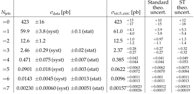
Table 3: Measured (σdata) and calculated cross sections of the production of Z+Njetsjets events.

The cross section calculated withMG5 aMCis given in the third column together with the total

7 0.00230

±

0.00060 (syst)

±

0.00051 (stat) 0.00157₋+0.00023_0.00026 +₋0.00012_0.00017 +₋0.00013_0.00019

6.3 Jet transverse momentum

Knowledge of the kinematics of SM events with large jet multiplicity is essential for the LHC experiments since these events are backgrounds to searches for new physics that predict decay chains of heavy coloured particles, such as squarks, gluinos, or heavy top quark partners. The

measured differential cross sections as a function of jet pT for the 1st, 2nd, 3rd, 4th, and 5thjets

are presented in Figs. 3–5. The cross sections fall rapidly with increasing pT. The cross section

for the leading jet is measured for pTvalues between 30 GeV and 1 TeV and decreases by more

than five orders of magnitude over this range. The cross section for the fifth jet is measured

for pT values between 30 and 100 GeV and decreases even faster, mainly because of the phase

space covered.

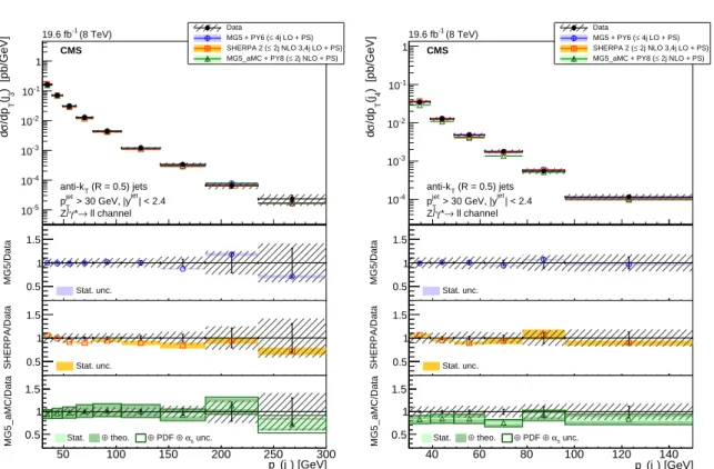
For the leading jet, the agreement of the MADGRAPH 5 + PYTHIA6 prediction with the

mea-surement is very good up to≈150 GeV. Discrepancies are observed from≈150 to ≈450 GeV.

A similar excess in the ratio with the tree-level calculation was observed at√s = 7 TeV in the

CMS measurement [8], using predictions from the same generators, as well as in the ATLAS

measurement [5], which used ALPGEN[48] interfaced toHERWIG[49] for the predictions. The

(13)

jets

N

= 0 = 1 = 2 = 3 = 4 = 5 = 6 = 7

-3 10 -2 10 -1 10 1 10 2 10 3 10 Data 4j LO + PS) ≤ MG5 + PY6 ( 2j NLO 3,4j LO + PS) ≤ SHERPA 2 ( 2j NLO + PS) ≤ MG5_aMC + PY8 ( CMS (8 TeV) -1 19.6 fb (R = 0.5) jets T anti-k | < 2.4 jet > 30 GeV, |y jet T p ll channel → * γ Z/ [pb] jets /dN σ d jets N = 0 = 1 = 2 = 3 = 4 = 5 = 6 = 7 MG5/Data 0.5 1 1.5 Stat. unc. jets N = 0 = 1 = 2 = 3 = 4 = 5 = 6 = 7 SHERPA/Data 0.5 1 1.5 Stat. unc. jets N = 0 = 1 = 2 = 3 = 4 = 5 = 6 = 7 MG5_aMC/Data 0.5 1 1.5

Stat. ⊕ theo. ⊕ PDF ⊕αs unc.

jets

N

0 ≥

≥

1 ≥

2 ≥

3 ≥

4 ≥

5 ≥

6 ≥

7

-3 10 -2 10 -1 10 1 10 2 10 3 10 Data 4j LO + PS) ≤ MG5 + PY6 ( 2j NLO 3,4j LO + PS) ≤ SHERPA 2 ( 2j NLO + PS) ≤ MG5_aMC + PY8 ( CMS (8 TeV) -1 19.6 fb (R = 0.5) jets T anti-k | < 2.4 jet > 30 GeV, |y jet T p ll channel → * γ Z/ [pb] jets /dN σ d jets N 0 ≥ ≥ 1 ≥ 2 ≥ 3 ≥ 4 ≥ 5 ≥ 6 ≥ 7 MG5/Data 0.5 1 1.5 Stat. unc. jets N 0 ≥ ≥ 1 ≥ 2 ≥ 3 ≥ 4 ≥ 5 ≥ 6 ≥ 7 SHERPA/Data 0.5 1 1.5 Stat. unc. jets N 0 ≥ ≥ 1 ≥ 2 ≥ 3 ≥ 4 ≥ 5 ≥ 6 ≥ 7 MG5_aMC/Data 0.5 1 1.5

Figure 2: The cross section for Z(→ ``) +jets production measured as a function of the (left)

exclusive and (right) inclusive jet multiplicity distributions compared to the predictions

calcu-lated with MADGRAPH5 +PYTHIA6,SHERPA2, andMG5 aMC+PYTHIA8. The lower panels

show the ratios of the theoretical predictions to the measurements. Error bars around the ex-perimental points show the statistical uncertainty, while the cross-hatched bands indicate the

statistical and systematic uncertainties added in quadrature. The boxes around theMG5 aMC

+PYTHIA8 to measurement ratio represent the uncertainty on the prediction, including

statis-tical, theoretical (from scale variations), and PDF uncertainties. The dark green area represents the statistical and theoretical uncertainties only, while the light green area represents the statis-tical uncertainty alone.

(14)

prediction fromSHERPA2 shows some disagreement with data in the low transverse

momen-tum region. The second jet shows similar behaviour. Both MADGRAPH 5 + PYTHIA 6 and

MG5 aMC + PYTHIA 8 are in good agreement with the measurement for the third jet pT

spec-trum. The shape predicted by the calculations from SHERPA 2 differs from the measurement

since the predicted spectrum is harder. For the 4thjet, the three predictions agree well with the

measurements. Calculations from SHERPA2 andMG5 aMC +PYTHIA8 predict different

spec-tra. Based on the experimental uncertainties it is difficult to arbitrate between the two, although we expect the one that includes four partons in the matrix elements to be more accurate. The

agreement ofSHERPA 2 and MADGRAPH 5 +PYTHIA 6 calculations with the measured 5thjet

pT spectrum is similar.

In summary, including many jet multiplicities in the matrix elements provides a good descrip-tion of the different jet transverse momentum spectra. Including NLO terms improves the agreement with the measured spectra. Nevertheless, some differences are observed between

the predictions calculated withSHERPA2 andMG5 aMC+PYTHIA8. The two calculations differ

in many ways, other than the fixed order: different PDF choices, different jet merging schemes,

and different showering models. In Ref. [8] it was shown that the jet pT spectra have little

de-pendence on the PDF choice, therefore the difference between the two generator is likely to be due to the different parton showerings or jet merging schemes.

) [GeV]

1

(j

T

p

-5 10 -4 10 -3 10 -2 10 -1 10 1 10 Data 4j LO + PS) ≤ MG5 + PY6 ( 2j NLO 3,4j LO + PS) ≤ SHERPA 2 ( 2j NLO + PS) ≤ MG5_aMC + PY8 ( CMS (8 TeV) -1 19.6 fb (R = 0.5) jets T anti-k | < 2.4 jet > 30 GeV, |y jet T p ll channel → * γ Z/ ) [pb/GeV] 1 (j T /dp σ d ) [GeV] 1 (j T p MG5/Data _0.5 1 1.5 Stat. unc. ) [GeV] 1 (j T p SHERPA/Data 0.5 1 1.5 Stat. unc. ) [GeV] 1 (j T p 100 200 300 400 500 600 700 800 900 1000 MG5_aMC/Data 0.5 1 1.5

) [GeV]

2

(j

T

p

-6 10 -5 10 -4 10 -3 10 -2 10 -1 10 1 10 Data 4j LO + PS) ≤ MG5 + PY6 ( 2j NLO 3,4j LO + PS) ≤ SHERPA 2 ( 2j NLO + PS) ≤ MG5_aMC + PY8 ( CMS (8 TeV) -1 19.6 fb (R = 0.5) jets T anti-k | < 2.4 jet > 30 GeV, |y jet T p ll channel → * γ Z/ ) [pb/GeV]2 (j T /dp σ d ) [GeV] 2 (j T p MG5/Data _0.5 1 1.5 Stat. unc. ) [GeV] 2 (j T p SHERPA/Data 0.5 1 1.5 Stat. unc. ) [GeV] 2 (j T p 100 200 300 400 500 600 700 800 MG5_aMC/Data 0.5 1 1.5

Figure 3: The differential cross section for Z(→ ``) +jets production measured as a function

of the (left) 1st_{and (right) 2}nd_{jet p}

Tcompared to the predictions calculated with MADGRAPH5

+ PYTHIA 6, SHERPA 2, and MG5 aMC + PYTHIA 8. The lower panels show the ratios of the

theoretical predictions to the measurements. Error bars around the experimental points show the statistical uncertainty, while the cross-hatched bands indicate the statistical and systematic

uncertainties added in quadrature. The boxes around the MG5 aMC + PYTHIA8 to

measure-ment ratio represent the uncertainty on the prediction, including statistical, theoretical (from scale variations), and PDF uncertainties. The dark green area represents the statistical and theoretical uncertainties only, while the light green area represents the statistical uncertainty alone.

T

p

-4 10 -3 10 -2 10 -1 10 Data 4j LO + PS) ≤ MG5 + PY6 ( 2j NLO 3,4j LO + PS) ≤ SHERPA 2 ( 2j NLO + PS) ≤ MG5_aMC + PY8 ( CMS (8 TeV) -1 19.6 fb (R = 0.5) jets T anti-k | < 2.4 jet > 30 GeV, |y jet T p ll channel → * γ Z/ ) [pb/GeV] ₅ (j _T /dp σ d ) [GeV] 5 (j T p MG5/Data 0.5 1 1.5 Stat. unc. ) [GeV] 5 (j T p SHERPA/Data 0.5 1 1.5 Stat. unc. ) [GeV] 5 (j T p 30 40 50 60 70 80 90 100 MG5_aMC/Data 0.5 1 1.5

Figure 5: The differential cross section for Z(→ ``) +jets production measured as a function of

the 5thjet pTcompared to the predictions calculated with MADGRAPH5 +PYTHIA6,SHERPA2,

andMG5 aMC +PYTHIA 8. The lower panels show the ratios of the theoretical predictions to

the measurements. Error bars around the experimental points show the statistical uncertainty, while the cross-hatched bands indicate the statistical and systematic uncertainties added in

quadrature. The boxes around the MG5 aMC + PYTHIA8 to measurement ratio represent the

uncertainty on the prediction, including statistical, theoretical (from scale variations), and PDF uncertainties. The dark green area represents the statistical and theoretical uncertainties only, while the light green area represents the statistical uncertainty alone.

(17)

6.4 Jet and Z boson rapidity

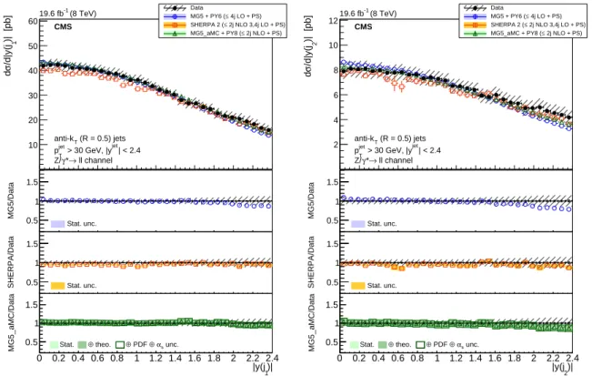
The differential cross sections as a function of the absolute rapidity of the first, second, third, fourth, and fifth jets are presented in Figs. 6, 7, and 8, including all events with at least one,

two, three, four, and five jets. The differential cross sections in |y|have similar shapes for all

jets while they vary by about a factor 2 in the range from 0 to 2.4.

The predictions obtained with SHERPA 2 provide the best overall description regarding the

shape of data distributions. The predictions of both MADGRAPH 5 +PYTHIA6 andMG5 aMC

+PYTHIA8 have a more central distribution than is measured for jets 1 to 4, although this

be-haviour is less pronounced for the latter. The difference could be attributed to the different showering methods and the different PDF choices for the three predictions. Given the

experi-mental uncertainties, the shape of the spectrum of the 5thjet rapidity is equally well described

by the three calculations.

)|

1

|y(j

)|

2

|y(j

of the (left) 1stand (right) 2ndjet|y|compared to the predictions calculated with MADGRAPH5

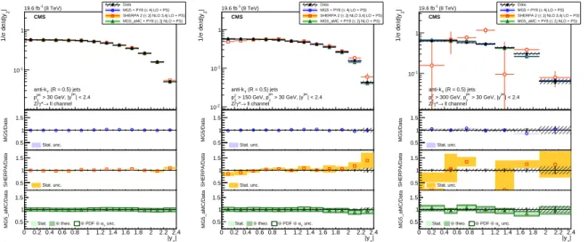
The Z boson rapidity distribution is presented in Fig. 9 with no requirement on the Z boson transverse momentum. To minimize the uncertainties the measurement is done for the normal-ized distributions. The relative contributions of matrix elements and parton shower depend on the Z transverse momentum. The measurement is also performed with a lower limit of 150 and

(18)

)|

3

|y(j

)|

4

|y(j

of the (left) 3rdand (right) 4thjet|y|compared to the predictions calculated with MADGRAPH5

(19)

)|

5

|y(j

Figure 8: The differential cross section for Z(→ ``) +jets production measured as a function of

the 5thjet|y|compared to the predictions calculated with MADGRAPH5 +PYTHIA6,SHERPA2,

(20)

300 GeV on the Z boson transverse momentum. Each distribution is normalised to unity. The three calculations are in very good agreement with the measured values. The agreement of the

prediction calculated withSHERPA 2 degrades when applying a threshold on the Z boson pT,

though it is still consistent with data within the statistical uncertainty.

| Z |y -1 10 1 Data 4j LO + PS) ≤ MG5 + PY6 ( 2j NLO 3,4j LO + PS) ≤ SHERPA 2 ( 2j NLO + PS) ≤ MG5_aMC + PY8 ( CMS (8 TeV) -1 19.6 fb (R = 0.5) jets T anti-k | < 2.4 jet > 30 GeV, |y jet T p ll channel → * γ Z/ | Z /d|y σ d σ 1/ | Z |y MG5/Data 0.5 1 1.5 Stat. unc. | Z |y SHERPA/Data 0.5 1 1.5 Stat. unc. | Z |y 0 0.2 0.4 0.6 0.8 1 1.2 1.4 1.6 1.8 2 2.2 2.4 MG5_aMC/Data 0.5 1 1.5

| Z |y -2 10 -1 10 1 Data 4j LO + PS) ≤ MG5 + PY6 ( 2j NLO 3,4j LO + PS) ≤ SHERPA 2 ( 2j NLO + PS) ≤ MG5_aMC + PY8 ( CMS (8 TeV) -1 19.6 fb (R = 0.5) jets T anti-k | < 2.4 jet > 30 GeV, |y jet T > 150 GeV, p Z T p ll channel → * γ Z/ | Z /d|y σ d σ 1/ | Z |y MG5/Data 0.5 1 1.5 Stat. unc. | Z |y SHERPA/Data 0.5 1 1.5 Stat. unc. | Z |y 0 0.2 0.4 0.6 0.8 1 1.2 1.4 1.6 1.8 2 2.2 2.4 MG5_aMC/Data 0.5 1 1.5

| Z |y -1 10 1 Data 4j LO + PS) ≤ MG5 + PY6 ( 2j NLO 3,4j LO + PS) ≤ SHERPA 2 ( 2j NLO + PS) ≤ MG5_aMC + PY8 ( CMS (8 TeV) -1 19.6 fb (R = 0.5) jets T anti-k | < 2.4 jet > 30 GeV, |y jet T > 300 GeV, p Z T p ll channel → * γ Z/ | Z /d|y σ d σ 1/ | Z |y MG5/Data 0.5 1 1.5 Stat. unc. | Z |y SHERPA/Data 0.5 1 1.5 Stat. unc. | Z |y 0 0.2 0.4 0.6 0.8 1 1.2 1.4 1.6 1.8 2 2.2 2.4 MG5_aMC/Data 0.5 1 1.5

Figure 9: The normalised differential cross section for Z(→ ``) +jets production measured as

a function of Z boson rapidity compared to the predictions calculated with MADGRAPH 5 +

PYTHIA6,SHERPA2, andMG5 aMC+PYTHIA8. The cross section is measured (left) inclusively

with respect to the Z boson pT, (middle) for pT > 150 GeV, and (right) for pT > 300 GeV. The

lower panels show the ratios of the theoretical predictions to the measurements. Error bars around the experimental points show the statistical uncertainty, while the cross-hatched bands indicate the statistical and systematic uncertainties added in quadrature. The boxes around the

MG5 aMC+PYTHIA8 to measurement ratio represent the uncertainty on the prediction,

includ-ing statistical, theoretical (from scale variations), and PDF uncertainties. The dark green area represents the statistical and theoretical uncertainties only, while the light green area represents the statistical uncertainty alone.

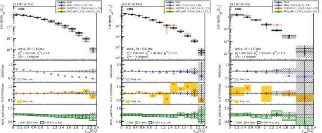
The correlations in rapidity between the different objects (Z boson and jets) are shown in Figs. 10 to 14. The normalised cross section is presented as a function of the rapidity difference

between the Z boson and the leading jet, ydiff(Z, j1) =0.5|y(Z) −y(j1)|in Fig. 10. A large

dis-crepancy is observed between the measured cross section and that predicted by MADGRAPH5

+PYTHIA6. Such an effect was previously observed at√s = 7 TeV [50] and is confirmed here

with an increased statistical precision and with an extended range in ydiff(Z, j1). The

discrep-ancy is significantly reduced when a threshold is applied to the transverse momentum of the Z boson as shown in the same figure. This observation supports the attribution of the discrep-ancy to the matching procedure between the ME and PS, as discussed in [50]. By contrast, a quite good agreement is found, independently of any threshold on the Z boson transverse

mo-mentum, for the NLO predictions ofSHERPA2, andMG5 aMC+PYTHIA8. This improvement

is expected to come from additional diagrams at NLO with a gluon propagator in the t-channel that populate the forward rapidity regions.

The presence of additional jets in the event should reduce the dependence on the ME/PS

matching for the first jet since this jet will have a larger pT on average. Figure 11 shows the

normalised cross section for Z production with at least two jets as a function of the

rapid-ity difference between the Z boson and the leading jet, ydiff(Z, j1), between the Z boson and

the second-leading jet, ydiff(Z, j2), and between the Z boson and the system formed by the

(21)

the MADGRAPH 5 +PYTHIA6 predictions are present in all three cases, but they are less pro-nounced than in the one-jet case (Fig. 11a compared to Fig. 10a). The NLO predictions from

SHERPA 2 andMG5 aMC +PYTHIA8 reproduce the measured dependencies much better than

MADGRAPH5 +PYTHIA6 does.

) 1 (Z,j diff y -3 10 -2 10 -1 10 1 Data 4j LO + PS) ≤ MG5 + PY6 ( 2j NLO 3,4j LO + PS) ≤ SHERPA 2 ( 2j NLO + PS) ≤ MG5_aMC + PY8 ( CMS (8 TeV) -1 19.6 fb (R = 0.5) jets T anti-k | < 2.4 jet > 30 GeV, |y jet T p ll channel → * γ Z/ )1 (Z,j diff /dy σ d σ 1/ ) 1 (Z,j diff y MG5/Data 0.5 1 1.5 Stat. unc. ) 1 (Z,j diff y SHERPA/Data 0.5 1 1.5 Stat. unc. ) 1 (Z,j diff y 0 0.2 0.4 0.6 0.8 1 1.2 1.4 1.6 1.8 2 2.2 2.4 MG5_aMC/Data 0.5 1 1.5

) 1 (Z,j diff y -4 10 -3 10 -2 10 -1 10 1 Data 4j LO + PS) ≤ MG5 + PY6 ( 2j NLO 3,4j LO + PS) ≤ SHERPA 2 ( 2j NLO + PS) ≤ MG5_aMC + PY8 ( CMS (8 TeV) -1 19.6 fb (R = 0.5) jets T anti-k | < 2.4 jet > 30 GeV, |y jet T > 150 GeV, p Z T p ll channel → * γ Z/ )1 (Z,j diff /dy σ d σ 1/ ) 1 (Z,j diff y MG5/Data 0.5 1 1.5 Stat. unc. ) 1 (Z,j diff y SHERPA/Data 0.5 1 1.5 Stat. unc. ) 1 (Z,j diff y 0 0.2 0.4 0.6 0.8 1 1.2 1.4 1.6 1.8 2 2.2 2.4 MG5_aMC/Data 0.5 1 1.5

) 1 (Z,j diff y -3 10 -2 10 -1 10 1 Data 4j LO + PS) ≤ MG5 + PY6 ( 2j NLO 3,4j LO + PS) ≤ SHERPA 2 ( 2j NLO + PS) ≤ MG5_aMC + PY8 ( CMS (8 TeV) -1 19.6 fb (R = 0.5) jets T anti-k | < 2.4 jet > 30 GeV, |y jet T > 300 GeV, p Z T p ll channel → * γ Z/ )1 (Z,j diff /dy σ d σ 1/ ) 1 (Z,j diff y MG5/Data 0.5 1 1.5 Stat. unc. ) 1 (Z,j diff y SHERPA/Data 0.5 1 1.5 Stat. unc. ) 1 (Z,j diff y 0 0.2 0.4 0.6 0.8 1 1.2 1.4 1.6 1.8 2 2.2 2.4 MG5_aMC/Data 0.5 1 1.5

Figure 10: The normalised differential cross section for Z(→ ``) +jets (Njets ≥1) production

measured as a function of the ydiffof the Z boson and the leading jet compared to the

predic-tions calculated with MADGRAPH5 +PYTHIA6,SHERPA2, andMG5 aMC+PYTHIA8. (left) The

cross section is measured inclusively with respect to the Z boson pTand for two different pT(Z)

thresholds. The ratio of the prediction to the measurements is shown for (left) pT > 0 GeV,

(middle) pT > 150 GeV, and (right) pT > 300 GeV. The lower panels show the ratios of the

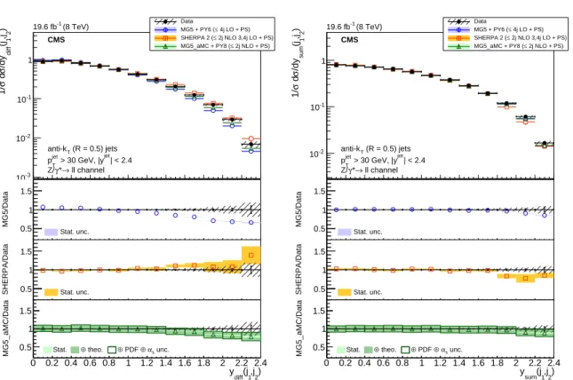
The rapidity correlation of the two leading jets, independently of the Z boson rapidity, is dis-played in Fig. 12, showing the rapidity sum and rapidity difference between the two jets. There is a good agreement between the measured cross section and the three predictions for the

ra-pidity sum dependence. The rara-pidity difference presents a discrepancy with MADGRAPH5 +

PYTHIA 6 at large values, while the NLO predictions ofSHERPA 2, and MG5 aMC +PYTHIA 8

are in good agreement with the data.

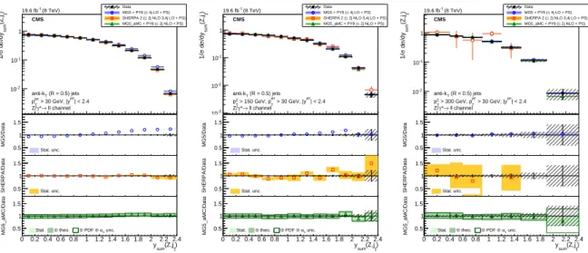
The rapidity sum for the system of the Z boson and the leading jet is studied with different thresholds applied to the transverse momentum of the Z boson. Figure 13 shows the nor-malised cross section as a function of the rapidity sum of the Z boson and the leading jet,

ysum(Z, j1) = 0.5|y(Z) +y(j1)|for Z boson transverse momentum above 0, 150, and 300 GeV.

The observed discrepancy between the measured cross section and that predicted by MAD

-GRAPH5 +PYTHIA6 is similar to the effect that has been found at 7 TeV [50], and is confirmed

here with increased statistical precision. The discrepancy almost vanishes when the transverse momentum of the Z boson is required to be larger than 150 GeV. The NLO predictions of

SHERPA 2, and MG5 aMC + PYTHIA8 are in good agreement with the measured cross section

independently of the Z boson transverse momentum. This improvement with respect to MAD

(22)

(Z,dijet) diff y -4 10 -3 10 -2 10 -1 10 1 Data 4j LO + PS) ≤ MG5 + PY6 ( 2j NLO 3,4j LO + PS) ≤ SHERPA 2 ( 2j NLO + PS) ≤ MG5_aMC + PY8 ( CMS (8 TeV) -1 19.6 fb (R = 0.5) jets T anti-k | < 2.4 jet > 30 GeV, |y jet T p ll channel → * γ Z/ (Z,dijet) diff /dy σ d σ 1/ (Z,dijet) diff y MG5/Data 0.5 1 1.5 Stat. unc. (Z,dijet) diff y SHERPA/Data 0.5 1 1.5 Stat. unc. (Z,dijet) diff y 0 0.2 0.4 0.6 0.8 1 1.2 1.4 1.6 1.8 2 2.2 2.4 MG5_aMC/Data 0.5 1 1.5

measured as a function of the ydiffof the Z boson and (left) the leading jet, (middle) the

second-leading jet, and (right) the system constituted by these two jets. The measurement is

com-pared to the predictions calculated with MADGRAPH 5 +PYTHIA 6,SHERPA 2, andMG5 aMC

+ PYTHIA 8. The lower panels show the ratios of the theoretical predictions to the

measure-ments. Error bars around the experimental points show the statistical uncertainty, while the cross-hatched bands indicate the statistical and systematic uncertainties added in quadrature.

The boxes around theMG5 aMC+PYTHIA8 to measurement ratio represent the uncertainty on

the prediction, including statistical, theoretical (from scale variations), and PDF uncertainties. The dark green area represents the statistical and theoretical uncertainties only, while the light green area represents the statistical uncertainty alone.

(23)

)

2

,j

1

(j

diff

y

-3 10 -2 10 -1 10 1 Data 4j LO + PS) ≤ MG5 + PY6 ( 2j NLO 3,4j LO + PS) ≤ SHERPA 2 ( 2j NLO + PS) ≤ MG5_aMC + PY8 ( CMS (8 TeV) -1 19.6 fb (R = 0.5) jets T anti-k | < 2.4 jet > 30 GeV, |y jet T p ll channel → * γ Z/ ) ₂ ,j 1 (j diff /dy σ d σ 1/ ) 2 ,j 1 (j diff y MG5/Data 0.5 1 1.5 Stat. unc. ) 2 ,j 1 (j diff y SHERPA/Data 0.5 1 1.5 Stat. unc. ) 2 ,j 1 (j diff y 0 0.2 0.4 0.6 0.8 1 1.2 1.4 1.6 1.8 2 2.2 2.4 MG5_aMC/Data 0.5 1 1.5

)

2

,j

1

(j

sum

y

-2 10 -1 10 1 Data 4j LO + PS) ≤ MG5 + PY6 ( 2j NLO 3,4j LO + PS) ≤ SHERPA 2 ( 2j NLO + PS) ≤ MG5_aMC + PY8 ( CMS (8 TeV) -1 19.6 fb (R = 0.5) jets T anti-k | < 2.4 jet > 30 GeV, |y jet T p ll channel → * γ Z/ ) ₂ ,j 1 (j sum /dy σ d σ 1/ ) 2 ,j 1 (j sum y MG5/Data 0.5 1 1.5 Stat. unc. ) 2 ,j 1 (j sum y SHERPA/Data 0.5 1 1.5 Stat. unc. ) 2 ,j 1 (j sum y 0 0.2 0.4 0.6 0.8 1 1.2 1.4 1.6 1.8 2 2.2 2.4 MG5_aMC/Data 0.5 1 1.5

measured as a function of the (left) ydiff and (right) ysum of the two leading jets. The

mea-surement is compared to the predictions calculated with MADGRAPH5 +PYTHIA6,SHERPA2,

(24)

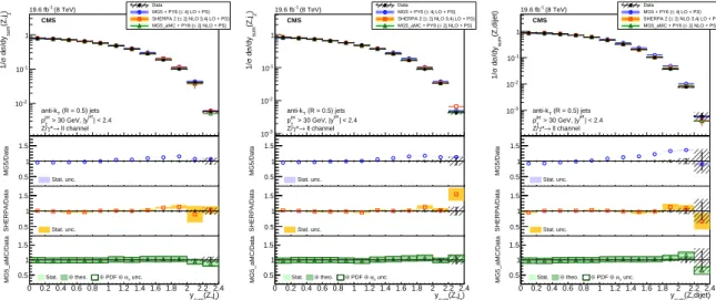
For dijet events, Fig. 14 shows cross sections as a function of rapidity sums, for the Z boson and the leading jet, for the Z boson and the second-leading jet, and for the Z boson and the dijet system of the two leading jets. Comparison between the measured cross sections and the

MADGRAPH5 + PYTHIA6 predictions exhibit a small disagreement for a rapidity sum above

1 for each jet, and the discrepancies increase when the dijet system is considered. Comparison

with NLO predictions from SHERPA 2, and from MG5 aMC + PYTHIA 8 shows a very good

agreement.

The rapidity correlation study confirms the observations made at√s = 7 TeV, and shows that

the behaviour with respect to the tree-level prediction is similar for the correlation with the second jet and enhanced when considering the dijet system consisting of the two leading jets. The study demonstrates that the two NLO predictions improve the agreement with the mea-surements, especially for the rapidity difference observables.

) 1 (Z,j sum y -2 10 -1 10 1 Data 4j LO + PS) ≤ MG5 + PY6 ( 2j NLO 3,4j LO + PS) ≤ SHERPA 2 ( 2j NLO + PS) ≤ MG5_aMC + PY8 ( CMS (8 TeV) -1 19.6 fb (R = 0.5) jets T anti-k | < 2.4 jet > 30 GeV, |y jet T p ll channel → * γ Z/ )1 (Z,j sum /dy σ d σ 1/ ) 1 (Z,j sum y MG5/Data 0.5 1 1.5 Stat. unc. ) 1 (Z,j sum y SHERPA/Data 0.5 1 1.5 Stat. unc. ) 1 (Z,j sum y 0 0.2 0.4 0.6 0.8 1 1.2 1.4 1.6 1.8 2 2.2 2.4 MG5_aMC/Data 0.5 1 1.5

) 1 (Z,j sum y -3 10 -2 10 -1 10 1 Data 4j LO + PS) ≤ MG5 + PY6 ( 2j NLO 3,4j LO + PS) ≤ SHERPA 2 ( 2j NLO + PS) ≤ MG5_aMC + PY8 ( CMS (8 TeV) -1 19.6 fb (R = 0.5) jets T anti-k | < 2.4 jet > 30 GeV, |y jet T > 150 GeV, p Z T p ll channel → * γ Z/ )1 (Z,j sum /dy σ d σ 1/ ) 1 (Z,j sum y MG5/Data 0.5 1 1.5 Stat. unc. ) 1 (Z,j sum y SHERPA/Data 0.5 1 1.5 Stat. unc. ) 1 (Z,j sum y 0 0.2 0.4 0.6 0.8 1 1.2 1.4 1.6 1.8 2 2.2 2.4 MG5_aMC/Data 0.5 1 1.5

) 1 (Z,j sum y -2 10 -1 10 1 Data 4j LO + PS) ≤ MG5 + PY6 ( 2j NLO 3,4j LO + PS) ≤ SHERPA 2 ( 2j NLO + PS) ≤ MG5_aMC + PY8 ( CMS (8 TeV) -1 19.6 fb (R = 0.5) jets T anti-k | < 2.4 jet > 30 GeV, |y jet T > 300 GeV, p Z T p ll channel → * γ Z/ )1 (Z,j sum /dy σ d σ 1/ ) 1 (Z,j sum y MG5/Data 0.5 1 1.5 Stat. unc. ) 1 (Z,j sum y SHERPA/Data 0.5 1 1.5 Stat. unc. ) 1 (Z,j sum y 0 0.2 0.4 0.6 0.8 1 1.2 1.4 1.6 1.8 2 2.2 2.4 MG5_aMC/Data 0.5 1 1.5

Figure 13: The normalised differential cross section for Z(→ ``) +jets (Njets ≥ 1) production

measured as a function of the ysum of the Z boson and the leading jet compared to the

pre-dictions calculated with MADGRAPH5 +PYTHIA6,SHERPA 2, andMG5 aMC+PYTHIA8. The

cross section is measured inclusively with respect to the Z boson pTand for two different pT(Z)

thresholds. The ratio of the prediction to the measurements is shown for (left) pT > 0 GeV,

(middle) pT > 150 GeV, and (right) pT > 300 GeV. The lower panels show the ratios of the

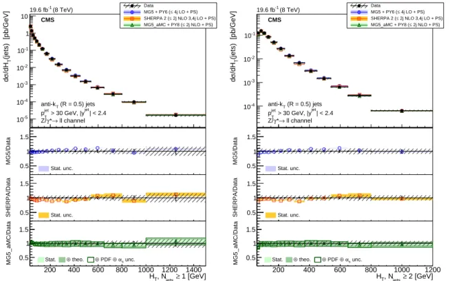
6.5 Differential cross section in jetHT

The hadronic activity of an event can be probed with the scalar sum of the transverse momenta

of the jets, HT. Measuring hadronic activity is important in searches for signatures with high

jet activity or, by contrast, when wishing to veto such activity, for instance in the central region when looking for vector boson fusion induced processes. In this section we present

measure-ments of the spectra for this variable in Z+jets events. The differential cross sections are shown