Rooftop photovoltaic potential analysis based on UAV-derived 3D-data and open source software

(1)

Rooftop Photovoltaic Potential Analysis based on

UAV-derived 3D-data and Open Source Software

Muhammad Gulraiz Khan

Academic research thesis submitted in partial fulfillment of the

requirements for the degree of:

Master of Science in Geospatial Technologies

Institute for Geoinformatics

2020

Westfälische Wilhelms-Universität

Münster, Germany

(2)

Declaration

I wrote this thesis on my own without the help of any other individual, I have listed all used references and sources and I did not submit this thesis to any other university.

Muhammad Gulraiz Khan Münster, Germany

Dated:

Name: Muhammad Gulraiz Khan WWU Matriculation Number: 500423 Email: [email protected]

Hosting university: University of Muenster

Supervisor: Dr. Torsten Prinz (University of Muenster) Co-supervisor 1: Christian Knoth (University of

Muenster)

(3)

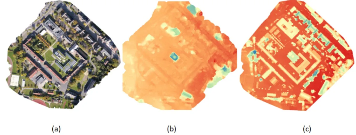
Figure 1. Leonardo Campus Muenster, Germany to be used as study area to test the GIS model. Variety of building rooftops available in the study area that will help to test model for different types of buildings. 11 Figure 2 (a) Modern building architecture with green flat rooftop (b) Traditional building in Germany with slanted rooftop. ... 12 Figure 3. UAV raw data collected by DJI Mavic pro with 80% overlapping of each tile. Overlapping of each image will provide good 3D point cloud due to stereo effect of each ground object. ... 12 Figure 4. Average monthly global irradiance data on horizontal surface for whole Germany with max. value of 222 kWh/sqr. Meter and min. value 169 kWh/ sqr.meter. ... 13 Figure 5. 3D point cloud density of UAV data that shows the clear shape and outline of a building. ... 14 Figure 6. . 3D point cloud density of laser scanning data that shows the clear shape and outline of a building. ... 14 Figure 7. Open drone map work flow from raw UAV data to resultant products using ODM and Docker. ... 15 Figure 8. Few of resultant products obtained after pre-processing of raw UAV images using Open Drone Map. (a) Orthophoto RGB mosaic, (b) Digital Terrain Model, (c) Digital Surface Model. ... 17 Figure 9. Conceptual design of GIS model showing input datasets for two parallel geoprocessing

workflows i.e rooftop extraction and solar energy calculation. ... 18 Figure 10. Usage of raster calculator tool to detect greenness in orthophoto, where “Orthophoto RGB” is the name of RGB imagery and @1, @2, @3 is the band number identification. ... 19 Figure 11. (a) Ortho-photo of the study area in RGB that was used to extract greenness (b) After applying the green band exaggeration equation on visible bands of orthophoto, the green parts are now can be distinguished. ... 20 Figure 12. Rooftop outline extraction QGIS model shows the work flow of getting input rasters and applying series of geoprocessing tools till the final results in the form of polygon. ...21

Figure 13. Illustration of earth rotation and seasonal variation throughout the year. It also shows the declination angles during different seasons. ... 22 Figure 14. Solar energy potential calculation workflow taking inputs in the form of raster datasets and numeric values of day and hour. After applying series of geoprocessing tools, the final raster was obtained where each pixel stores the solar potential value. ...24

(5)

5 | P a g e Figure 15. Combining both modules (Rooftop extraction and solar energy calculation) in one QGIS workflow that shares inputs. ... 25 Figure 16. (a) Rooftop outlines extracted from UAV 3D data and ortho-photo. (b) Rooftop outlines extracted from laser scanning 3D data and multi-spectral ortho-photo. ...27 Figure 17. Model precision to detect the rooftop lining even the data is missing. (a) Shows UAV data missing on the edges but model detected the outline according to the availability and quality of data. (a) Same building from Lidar data with complete outline. ...28 Figure 18. (a) Solar energy potential for whole study area derived from UAV. (b) Solar energy potential derived from laser scanning data. ... 29 Figure 19. (a) Solar energy potential for extracted rooftops derived from UAV. (b) Solar energy potential derived from laser scanning data. ... 30 Figure 20. Rooftop area comparison of Lidar and UAV data with manually digitized polygon. Horizontal axis show unique building ID and vertical axis shows area in square meters. ... 32 Figure 21. (a) Shows percentage of difference in rooftop area for Lidar driven extraction with reference to manually digitized outlines. Green line shows the average difference for all buildings. (b) Shows

percentage of difference in rooftop area for UAV driven extraction with reference to manually digitized outlines. Green line shows the average difference for all buildings. ... 32 Figure 22. (a) Shows comparison between UAV and Lidar driven solar energy potential. (b) Shows average difference for all buildings in red straight line and percentage difference of each building in blue bars. ... 33

List of Tables

Table 1. Solar energy potential comparison of study area for both UAV and Lidar data, shows maximum and minimum value in kWh/sqr. meter, total sum of energy and mean & standard deviation. ... 29 Table 2. Solar energy potential comparison of extracted rooftops for both UAV and Lidar data, shows maximum and minimum value in kWh/sqr. meter, total sum of energy and mean & standard deviation. . 30 Table 3. Detailed rooftop area comparison for each individual building with unique id in terms of actual difference in square meters as well as percentage difference. ... 31 Table 4. Solar energy potential in kilo Watt Hour (kWh) for each individual building derived from UAV and Lidar an average difference between two for same rooftop. ... 33

(6)

6 | P a g e List of Equations r =_{𝑅𝑅 + 𝐺𝐺 + 𝐵𝐵 , g =}𝑅𝑅 _{𝑅𝑅 + 𝐺𝐺 + 𝐵𝐵 , b}𝐺𝐺 =_{𝑅𝑅 + 𝐺𝐺 + 𝐵𝐵}𝐵𝐵 ……… 19 𝐸𝐸𝐸𝐸𝐺𝐺 = 2g − 𝑟𝑟 − 𝑏𝑏 ……… 19 S ↓ = S cos i ……… 22

cos i = cos α cos z + sin α sin z (a − b) ……… 22

z = cos−1_{(sin ∅ sin δ + cos ∅ cos δ cos h)} _{……… 22}

a = cos−1₍cos z sin ∅ − sinδ sin z cos ∅ ……… 23

(7)

7 | P a g e Abstract: Electric energy is one of the driving forces for economic growth. Energy supply to rural areas is a big challenge for many countries, especially for those with less income and sparse settlements where main grid supply is not feasible. Solar energy is the most abundant, clean and readily available natural energy source. Open source technology and low cost UAV data can be used to assess solar potential on rooftops so that main grid supply will not be required for small settlements. This research aimed to develop procedures and workflows to address this problem. A test site in Muenster WWU (Leonardo campus) was used to test the model because both UAV and highly accurate laser scanning data are readily available. Solar global irradiance data was also available for Germany. After pre-processing of raw UAV images, rooftop extraction model was designed to extract rooftops using RGB images and 3D data. Solar energy calculation model was used to compute the potential for each raster pixel for extracted rooftops. Open Drone Map, Docker and QGIS were all open source software used to run this workflow. This model can be implemented on different regions under some constraints. Accuracy assessment gave insight of the accuracy of this GIS model, so that future improvements can be made.

1 Introduction

One of the Key factors in the economic growth of any country is energy, to be more specific, it is electrical energy that drives the economy (Hamdi, Sbia, & Shahbaz, 2014). Energy generation from fossil fuels is not a cheap solution; it comes with a financial cost as well as the environmental cost. Due to higher prices of crude oil, energy production remains a big challenge for under developed countries (Baffes, et al. 2015). Countries with less natural resources and limited capacity of managing the energy sector are facing severe energy shortfall. Dispersed settlements are one of the main affectees of electricity deficiencies because of the distance from national grid, lack of infrastructure and limited financial resources of governments. Access to electricity will bring the rural population in main stream and it will be beneficial for the economy of the country.(Melkior, Tlustý & Müller, 2016).

Standalone electric power solution for sparse rural areas can be beneficial for both residents and governing authorities because there will be less need of infrastructure to be developed for electrification and also there will be no ne ed to deploy administrative and technical staff for operations and maintenance. Un-electrified rural areas need a low cost and environment friendly solution; installation of photovoltaic (PV) modules on rooftops is a convenient method to address this problem. Levelized cost of solar energy is also decreasing with the advancement in PV cells

(8)

8 | P a g e

production technology and increased production capacity. There was an 80% decrease in cent/kWh in electricity production using PV cells from 2005 to 2015 according to a study conducted by Agora Energiewende, Germany published in 2015, making it possible to replace hydrocarbons fuels (Fraunhofer ISE, 2015).

Rooftop solar energy solution is also equally beneficial for already electrified settlements using feed-in management of electricity in which the consumer can feed the main grid with solar energy which is not being consumed. For example feed-in management is legally allowed in Germany as per German Renewable Energy Sources Act EEG 2009 and consumers can install PV modules to export solar energy to national grid (Braun, Perrin & Feng, 2009). Rooftop PV installation is very efficient in terms of time required to install the modules and also scalable to increase solar energy production by involving residents of the country and without spending tax payer’s money on big solar power plants.

Government or funding agencies should know the estimated installation potential of solar PV in any settlement to allocate funds. Secondly general public can also use these estimations to assess the solar potential for self funding. This study aims to find the cost effective technological solution that can give a clear picture to the authorities as well as to the general public, helping them in taking decisions. This model tends to focus on under-developed countries or developing countries as a first step to achieve their energy needs that is why low cost drone images and open source software is being proposed.

This research thesis will focus on solar potential analysis using open source geo-spatial technologies and 3D data derived from low cost drones. The result of this research is expected to find cost effective approach to accomplish this task. For testing and analysing different methodologies,WWU Leonardo campus in Muenster, Germany will be chosen as study area.

1.1 Problem Statement and Research Question

Investigation of roof top solar energy potential in terms of availability of suitable area with respect to solar insolation, orientation, slope, aspect and shade, using dense 3D point cloud data from low cost UAV platform using open source technologies is much needed for small settlements that are not connected with the national grid in under developed countries.

Detailed and workable GIS workflow needs to be developed to tackle this problem. Proprietary software and solutions provide off the shelf solutions but they are costly and not much flexible in

(9)

9 | P a g e

terms of modification. Complete workflow from raw UAV data processing to final spatial analysis results, which will provide insight of solar potential over the rooftops is in need for low income countries with sparse population.

This research thesis will attempt to develop a GIS model to tackle this problem and will try to answer following research question and sub-questions.

How does a low cost high resolution UAV data can be used to assess the roof top solar energy potential using open source software?

• What is the accuracy of results as compared to highly quality laser scanning? • How can this model be applicable on different regions?

2 Methodological Background

Use of geo-spatial technologies to seek smart solutions for complex decision making problems is a new approach and making decision makers smarter than before. Geographical aspect enables us to study environmental problems more deeply. To study geographical phenomena, spatial data is needed to be acquired using different platforms according to the needs of project.

Use of open source GIS tools to determine photovoltaic potential in urban area of city of Bardejov in eastern Slovakia gave the result for 1440 bui ldings which can produce approximately 25GWh electric power annually, which is 45 percent of annual requirement of electricity in year 2008 (Hofierka & Kaňuk, 2009). 3D city model creation implemented in GIS database requires Digital Terrain Model (DTM), Digital Elevation Model (DEM) and Digital Surface Model that plays key role in 3D analysis of roof top extraction. These datasets can easily be obtained from drone aerial images along with 3D point cloud (Padró et al., 2019). Due to advancement in the drone technologies and development of various image analysis software cost of aerial remote sensing is substantially reducing (P.Urbanová, M.Jurda & T. Vojtisek, 2017). Lidar data for creating 3D point clouds is being employed in various applications and also the photogrammetric image matching techniques are not new to generate quick point clouds (Nex & Rinaudo, 2011). Lidar provides highly accurate data but it is beyond the cost of many small projects with low budgets. According to the project scope and required outcomes, any of these technologies can be chosen but for this kind of project where very large area coverage is required, a cost effective and fast solution should be appreciated.

(10)

10 | P a g e

UAV point cloud data cannot provide 3D points under the surface like trees. Depending upon application area, if only surfaces are being studied e.g. roof tops in current context, then low cost UAV 3D data can easily be incorporated (Cao et al., 2019).

Many countries, facing electric power shortfall, have started net-metering or self-consumption of electric energy e.g. Pakistan in 2015, where consumers can install their own solar modules on roof tops and can inject electric power in national grid, at the end of the month they receive net bill after the compensation of exported electricity (AEDB). Solar energy is one of the most abundant natural energy sources that need to be harnessed, importance can be judged by number of projects that have been launched, completed and under progress worldwide from all around the world. Energy Sector Management Assistance Program by world bank is one big example where 18 donors including European Union and Germany are working together for renewable energy potential in the world including solar energy (Stökler, Schillings & Kraas, 2016). Costly solutions to analyse solar potential is acceptable neither by developing countries and nor by the developed countries if our main goal is achievable with less expense.

Digital terrain model and digital surface model can be derived from LIDAR data which was available in ASCII format and usually divided into geographic tiles for easy handling due to massive size of data. Use of LIDAR data for 3D analysis of urban area to calculate solar power potential in Auckland is a technologically wise choice (Suomalainen, Wang & Sharp, 2016). Multi spectral Quick Bird imagery was used to extract bright rooftops to calculate solar potential in Bangladesh with 60cm spatial resolution (Kabir, Endlicher & Jägermeyr, 2010).

Accurate roof top extraction is the most critical part according to above literature review. High resolution multi-spectral satellite imagery had been used to extract bright rooftops on the basis of spectral signatures. Satellite imagery can only retrieve flat surface and do not include any 3D information to describe the orientation and slope of the roof. Lidar data to find rooftop solar potential was used in Germany and New Zeeland by generating Digital Surface Model which provides the 3D roof tops providing slopes and orientation. With the help of this data, solar insolation can be determined on different parts of the roof, that ultimately will help to find suitable spots to install solar PV modules (Suomalainen et al., 2016). Using digital aerial photogrammetry point clouds for 3D analysis to extract roof tops is a new concept and not

(11)

11 | P a g e

experimented before. Comparison of point clouds from aerial photogrammetry with Lidar will determine that if it is possible to use low cost aerial platforms instead of costly Lidar survey.

3 Materials and Methods

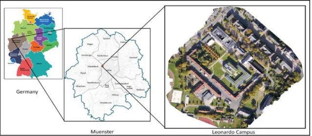
3.1 Study Area

Testing and validation of the spatial model for rooftop solar energy potential assessment was carried out over the selected study area of Leonardo Campus located in University of Muenster (WWU), Muenster, Germany as shown in Figure1. The centroid of study area is at Latitude 51.975 and Longitude: 7.601. Area covered by drone was 0.15 km2_.

Figure 1. Leonardo Campus Muenster, Germany to be used as study area to test the GIS model. Variety of building

rooftops available in the study area that will help to test model for different types of buildings.

Availability of various types of roof tops e.g. slanted, flat and green is a good reason to choose this study area to test the model. There are different types of buildings as well, like single story, multi-storey, small and large buildings. Figure2 shows the green flat rooftop as well as the traditional rooftop in Germany. Vegetation cover of grass, plants and trees is also available in selected area; also laser scanning data is freely available along with multispectral high resolution orthophoto that was used for accuracy assessment of results of the developed model.

(12)

12 | P a g e

Figure 2 (a) Modern building architecture with green flat rooftop (b) Traditional building in Germany with slanted

rooftop.

3.2 Data Sets

3.2.1 UAV Aerial Data

Aerial photographs were acquired using DJI Mavic pro drone that is considered as a low cost drone from Chinese origin. This drone can capture images only in RGB bands with 12.35 megapixels and there is no pr ovision to install any other sensor like NIR that helps to detect vegetation. Maximum image size is 4000 × 3000 pixels and image format is JPEG (DJI, 2019). 80 percent overlapping for each consecutive image was adopted to generate dense and detailed 3D point cloud (DroneDeploy, 2019). Figure3 shows the UAV images that were collected in summer season June 2019 with 60 meters altitude from ground surface. Spatial resolution of the collected imagery was 5cm. 507 overlapping images were collected for the study area.

Figure 3. UAV raw data collected by DJI Mavic pro with 80% overlapping of each tile. Overlapping of each image will

(13)

13 | P a g e

3.2.2 Global Solar Data

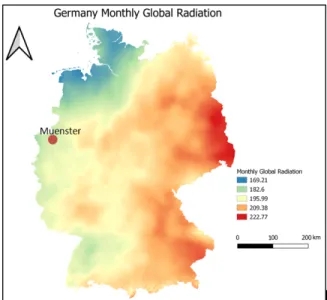
Solar insolation data for Germany in Figure4 was acquired from German meteorological deportment (Deutscher, 2019) .This data archive provides number of datasets including Global solar irradiance which provides average short-wave radiation intensity reaching on horizontal surfaces. Average monthly data is available since 1991 till date. Final product of monthly average global solar data is obtained by merging ground stations data and satellite radiation data to provide more accuracy. Datasets were provided in ASCII Raster format with spatial resolution of 1km x 1km. Unit of pixel value is kWh/m2. To test the model latest dataset for June 2019 were acquired.

Figure 4. Average monthly global irradiance data on horizontal surface for whole Germany with max. value of 222

kWh/sqr. Meter and min. value 169 kWh/ sqr.meter.

3.2.3 LIDAR and Multispectral Data

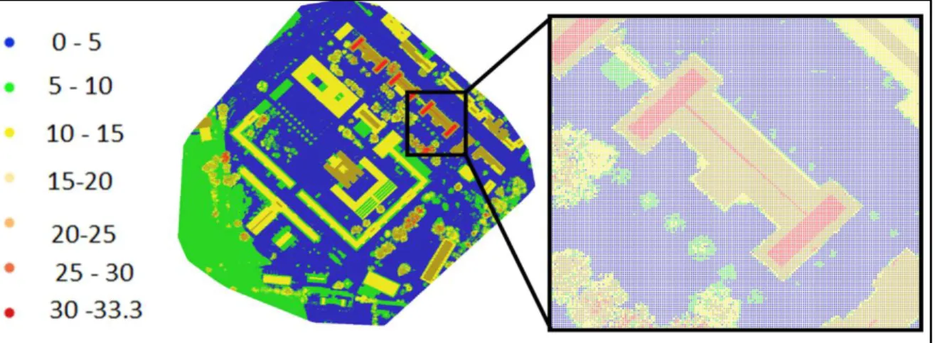
Large number of different datasets is available on official geo-portal of Nordrhein Westfalen state, where the study area exists. Open data can be freely downloaded using various selection tools available on geo-viewer with user friendly user interface. Digital Surface Model for study area was originally captured using aircraft based laser scanning that is readily available on geo-portal in XYZ format. Figure 5 shows point cloud data, that has been recorded with a point density of at least four points per square meter. Reference system of the downloaded data was EPSG: 25832 (Geoportal NRW, 2019).

(14)

14 | P a g e

Figure 5. 3D point cloud density of UAV data that shows the clear shape and outline of a building.

High resolution orthophoto was available for study area with spatial resolution of 10cm per pixel, that can be seen in Figure 6. This imagery is multispectral, RGB and near infrared (RGBNIR). Only RGB channels were used for testing the model as UAV data was only captured in RGB without near infrared sensor. These orthophotos are updated every 3 years. Last update was available on 31 July 2019. Reference system of the downloaded imagery was EPSG: 25832 and raster format was JPEG2000 (Geoportal NRW, 2019).

Figure 6. . 3D point cloud density of laser scanning data that shows the clear shape and outline of a building in

(15)

15 | P a g e 3.3 Data Processing

Before designing and development of spatial model; processing of raw UAV Images was required to generate Orthophoto, Digital Surface Model and Digital Terrain Model.

Open source technologies were adopted for all pre-processing, data cleaning, analysis, and post-processing procedures. Following software and libraries were used to setup the experimental environment.

• Docker 2.1.0.5 for Windows

• Open Drone Map

• QGIS 3.8

• GDAL

3.3.1 Docker

Windows 10 64-bit Educational edition was used to install Docker. Docker can be run only on Pro, Enterprise and Educational edition of Windows operating system. Hyper-V for virtualization and containers windows feature were enabled by default but before proceeding to installation, it was confirmed. There were some basic system requirements e.g. 64 bit processor and 4 GB RAM but after practical experience and considering the size of data to be processed, at least 16 GB RAM is recommended and also used the same in this project (Docker, 2019).

3.3.2 ODM Process in Docker

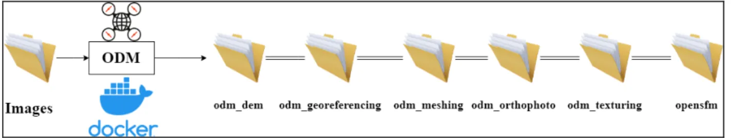
Open Drone Map (ODM) was used to generate orthophotos and 3D data products from raw drone images. ODM has two versions, one has web interface is called WebODM and other is ODM for Docker. ODM Docker image provides more control on s etting the parameters. To initialize the process, Input and output directories need to be created. Figure 7 shows the process workflow and output folder structure.

(16)

16 | P a g e

Batch file runs commands to automate the process, Code 1 shows how should the old directories be removed each time before creating the directory structure. Windows command line can be used to execute several commands to execute the process, batch file can also be created that stores all command script in a sequential manner so that each time user can execute the process just by running the script file, this will automate the process (Microsoft, 2019).

1. @echo off 2. rmdir odm_georeferencing /s /q 3. rmdir odm_orthophoto /s /q 4. rmdir odm_texturing /s /q 5. rmdir odm_meshing /s /q 6. rmdir opensfm /s /q 7. rmdir odm_dem /s /q 8. mkdir odm_georeferencing 9. mkdir odm_orthophoto 10. mkdir odm_texturing 11. mkdir odm_meshing 12. mkdir opensfm 13. mkdir odm_dem 14. echo %cd%

Code 1.Removing existing folder structure if exist and creating new directories without containing any files.

After creation of required directory structure, ODM command can be run using Docker commands. Docker commands can be run from any file location but to make it simpler, current directory was used. First part of command in Code 2 is the standard docker parameters and input of raw UAV images. Second part is dedicated for storing output results and the last part is dedicated for pulling the Docker image for ODM from images repository with additional parameters for 3D data outputs i.e.--dsm –dtm.

1. docker run -it --rm -v "%cd%\images:/code/images" -v "%cd%\odm_orthophoto:/code/odm_orthophoto" -v "%cd%\odm_texturing:/code/odm_texturing" -v "%cd%\odm_meshing:/code/odm_meshing" -v

"%cd%\odm_georeferencing:/code/odm_georeferencing" -v "%cd%\opensfm:/code/opensfm" -v "%cd%\odm_dem:/code/odm_dem" opendronemap/odm --dsm --dtm

Code 2. Standard format of docker command to read input images and after processing storing the results in designated

folders by calling Open Drone Map Docker image.

3.3.3 Open Drone Map Output

Open Drone Map generates multiple data products in various data formats. Mainly three data sets extracted from UAV data were used in the GIS model: Figure 8(a) is the orthophoto that was used to extract greenness of the area because on later steps, vegetation should be excluded.

(17)

17 | P a g e

Figure 8(b) is the Digital Terrain Model and Figure 8(c) is the Digital Surface Model to distinguish between ground features and non-ground features e.g. buildings and trees.

Figure 8. Few of resultant products obtained after pre-processing of raw UAV images using Open Drone Map. (a)

Orthophoto RGB mosaic, (b) Digital Terrain Model, (c) Digital Surface Model.

3.3.4 Harmonization of Datasets

All datasets required as inputs of QGIS model needed to be on same spatial reference that is EPSG: 32632 - WGS 84 / UTM zone 32N and clipped precisely for study area. All inputs were in raster format so spatial resolution was also adjusted to 5cm while using in QGIS model. Model was run two times for the same study area, firstly for drone data and secondly for Lidar. Both types of inputs were prepared on single standard. Latitude raster with latitude value was stored in each pixel and monthly average solar incident raster on horizontal surface were same for both runs. Ortho-photo, DSM and DTM for both Lidar and UAV data were on same reference system and same spatial resolution.

3.4 Model Design

QGIS 3.8 gives the provision to design spatial model using graphical modeller. Geoprocessing tools and algorithms can be linked together to generate an automated workflow. Graphical modeller provides the designing capability to implement the GIS model Logic. Inputs can be set for user in the form of raster datasets, vector datasets and also the numerical values. Raster calculator, Slope, Aspect, GDAL Sieve, Polygonization, Simplify edges, Extract raster by polygon and Zonal statistics tools were used frequently in the GIS model.

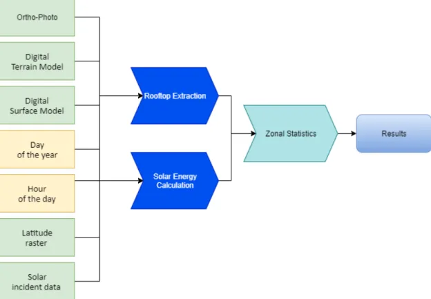
Logical conceptual design that was prepared before dive into actual processing model can be seen in Figure 9. There were two parallel processes with combined inputs i.e. rooftop extraction and solar energy calculation, that were combined at the end to get final results. Seven inputs

(18)

18 | P a g e

were required to feed in the model including Ortho-photo, Digital Terrain Model (DTM), Digital Surface Model (DSM), Day of the year, Hour of the same day, Latitude raster and Solar incident data on horizontal surface. After Rooftop extraction and solar energy calculation for study area, solar energy potential was calculated for each building rooftop for one particular day and one particular hour that were given as input. Same model design is valid for both UAV data and Lidar data with correct changes in parameter values according to the study area and data.

Figure 9. Conceptual design of GIS model showing input datasets for two parallel geoprocessing workflows i.e rooftop

extraction and solar energy calculation.

3.5 Rooftop Extraction

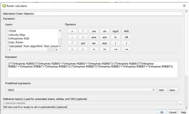
Rooftop extraction part of the model accepts three inputs i.e. DTM, DSM and Ortho-photo. Ortho-photo was used to detect green parts of the image because near infrared sensor was not used. Green band of the RGB photo was enhanced to get the excess green index (Yang, et al. 2015). Normalized values for each band were required and were calculated using equation (1). Where R,G,B are the bands of ortho-photo and r,g,b are normalized values of red, green and blue. Equation (2) was used to enhance the green pixels to be extracted.

(19)

19 | P a g e r =_{𝑅𝑅 + 𝐺𝐺 + 𝐵𝐵 , g =}𝑅𝑅 _{𝑅𝑅 + 𝐺𝐺 + 𝐵𝐵 , b =}𝐺𝐺 _{𝑅𝑅 + 𝐺𝐺 + 𝐵𝐵}𝐵𝐵 (1)

𝐸𝐸𝐸𝐸𝐺𝐺 = 2g − 𝑟𝑟 − 𝑏𝑏 (2)

Figure 10 shows the actual implementation of equation 1 and 2 in QGIS raster calculator tool where each RGB band was used as a variable of equation. Figure 11(b) shows the result of green extraction method, where enhance green pixels are shown in green and all other pixels are shown in black

Figure 10. Usage of raster calculator tool to detect greenness in orthophoto, where “Orthophoto RGB” is the name of

(20)

20 | P a g e

Figure 11. (a) Ortho-photo of the study area in RGB that was used to extract greenness (b) After applying the green band

exaggeration equation on visible bands of orthophoto, the green parts are now can be distinguished.

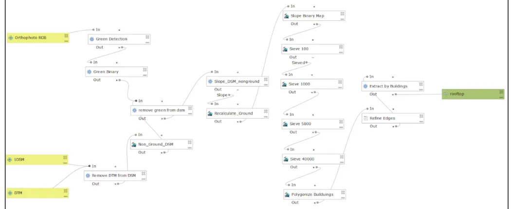
Figure 12 s hows the QGIS workflow for extraction of rooftops. DTM, DSM and orthophoto were used as inputs for the workflow. First step was to distinguish between features on ground and non-ground features. Non-ground features are defined as the features elevated from ground surface e.g. trees, buildings and other manmade features. Difference between DTM and DSM values gives the elevation difference that can be used to identify non-ground features. To distinguish between trees and building, ExG raster generated using equation 2 was subtracted from non-ground features and additionally the features with lesser slope helped to distinguish buildings. Applying the threshold values according to the data, binary map of ground and non-ground was generated. All pixels having greater elevation than set threshold value were assigned 1 value and the features having less value than set threshold were set to 0. There were many small scattered patches of elevated features that were needed to be excluded. Sieving process on resultant binary raster eliminated the small unwanted pixel clusters. As a result clean binary map of 0 and 1 values was obtained. Polygonization of this raster grouped the pixels together and provided vectorized data for each building rooftop.

(21)

21 | P a g e

Figure 12. Rooftop outline extraction QGIS model shows the work flow of getting input rasters and applying series of geoprocessing tools till the final results in the form of

(22)

22 | P a g e 3.6 Solar Energy Calculations

Solar energy calculation over the rooftops depends upon many factors because of earth rotation. Illustration in Figure 13 de picts seasons around the year are changed due to summer solstice (June 21 or 22), winter solstice (December 21 or 22), vernal equinox (21 March) and autumnal equinox (September 22 or 23). It also changes the declination of axis of earth.

Figure 13. Illustration of earth rotation and seasonal variation throughout the year. It also shows the declination angles

during different seasons.

Solar irradiance in Equation 3 over the tilted rooftops is the product of solar irradiance on flat surface and cosine of angle of incidence between sun and normal to the rooftop surface weather it is tilted or flat.

S ↓ = S cos i (3)

Where S↓ is solar irradiance over the rooftop, S is solar irradiance on flat surface and i is the angle of incidence. Angle of incidence depends upon s lope of rooftop, zenith angle of sun, azimuth of sun and azimuth of surface. It can be calculated using Equation 4.

cos i = cos α cos z + sin α sin z (a − b) (4)

Where α is slope of rooftop, z is solar zenith, a is azimuth angle of sun and b i s azimuth of rooftop. Slope and azimuth of rooftops can be calculated using geoprocessing tools directly from digital surface model. Solar zenith angle z can be calculated using Equation 5.

(23)

23 | P a g e

Where ø is latitude value of the particular pixel, δ is solar declination angle and h is hour angle of the sun. Solar azimuth angle is the angle between north and the projection of sun on t he horizontal plane. It can be calculated using Equation 6.

a = cos−1₍cos z sin ∅ − sinδ

sin z cos ∅ )

(6)

Five inputs as shown in Figure 14 were required to calculate solar energy; three of them were raster datasets i.e. solar data for study area, digital surface model and latitude raster. Two inputs were numeric variables for day and hour when the energy was being calculated. DSM was used as input of aspect and slope tools. Declination of sun for a specific day of the year was calculated using numeric value of day of the year and DSM to generate raster for further usage. Hour angle calculation was quite straight forward which took hour as input and used DSM to generate raster. Declination angle and hour angle along with latitude raster were used as input to calculate solar zenith angle. The same declination and hour angles were used to calculate solar azimuth where previously calculated zenith angle was also used as input. Finally incident angle was calculated and multiplied with solar data which gives the final raster showing solar energy potential per square meter per pixel.

3.7 Final QGIS Model

Rooftop extraction and solar data calculation were two separate processes in QGIS sharing some input datasets. Both processes run parallel to provide building rooftop outlines and solar energy potential on each pixel in kWh/m2_{and join together for zonal statistics tool as shown in Figure}

15. This tool extracts pixel values from solar energy raster to each respective polygon. It provides various statistical values for each building e.g. Pixel count, Sum of values and average of values. This combined QGIS model will facilitate the end user by providing an interactive graphical user interface so that the end user will only set input data sets of digital terrain model, digital surface model, orthophoto, solar incident data, and latitude values in raster format. Numeric values will be input as Day of the year and hour of the day.

(24)

24 | P a g e

Figure 14. Solar energy potential calculation workflow taking inputs in the form of raster datasets and numeric values of day and hour. After applying series of geoprocessing

(25)

25 | P a g e

(26)

26 | P a g e

4 Results

4.1 Rooftops Extracted from UAV and Lidar Data

UAV RGB data, DSM and DTM can be used to extract rooftop outlines and open source software QGIS and Open Drone Map run required geo-processing tools standalone as well as in a model workflow. Results of rooftop outline from both data acquisition methods using same geo-processing model do not have drastic differences as it can be seen in Figure 16 (a) & ((b). The developed GIS model can detect the edges very efficiently depending upon the quality of data in terms of spatial resolution and elevation precision for 3D data for DSM and DTM. Figure 17 shows if the data is missing somewhere in the image then the outline will be drawn accordingly.

(27)

27 | P a g e

(28)

28 | P a g e

Figure 17. Model precision to detect the rooftop lining even the data is missing. (a) Shows UAV data missing on the edges but model detected the outline according to the

(29)

29 | P a g e 4.2 Solar Energy Potential Derived from UAV and Lidar Data

Solar global incident data on horizontal surface provided solar energy potential on flat surface for whole study area without considering any features on surface of earth but when manmade and natural features were considered then the solar incident angle came into play and provided solar energy potential over the surfaces of these features as well as on ground.

Table 1. Solar energy potential comparison of study area for both UAV and Lidar data, shows maximum and minimum

value in kWh/sqr. meter, total sum of energy and mean & standard deviation.

UAV data Lidar data Difference Minimum value(kWh/m2₎ _-0.24 _-0.14 _-0.1

Maximum value(kWh/m2₎ _0.30 _0.30 ₀

Sum 8,166,222.3 12,235,370.4 4,069,148.1 Mean value(kWh/m2₎ _0.139 _0.207 _0.068

Standard deviation 0.100 0.103 0.003

Table 1 gives the information about standard deviation that shows the relative characteristics of both datasets and within the same dataset values of solar potential at pixel level are changing with same proportion for both UAV and Lidar. Difference in sums of potential for whole study area is about 33% which shows the difference of data quality with respect to each other. Visible difference can be seen in Figure 18 (a) and (b).

Figure 18. (a) Solar energy potential for whole study area derived from UAV. (b) Solar energy potential derived from

(30)

30 | P a g e

Figure 18 shows whole area under consideration, to go down further for only rooftops according to the research question shows clearer picture. Following table shows the values of solar energy potential only for rooftops.

Table 2. Solar energy potential comparison of extracted rooftops for both UAV and Lidar data, shows maximum and

minimum value in kWh/sqr. meter, total sum of energy and mean & standard deviation.

UAV data Lidar data Difference Minimum value(kWh/m2₎ _-0.24 _-0.14 _-0.1

Maximum value(kWh/m2₎ _0.30 _0.30 ₀

Sum 1,617,604.3 2,364,076.7 746,472.4 Mean value(kWh/m2₎ _0.134 _0.208 _0.074

Standard deviation 0.107 0.080 0.027

Unlike the previous rooftop results, it can be seen in Table 2 that the standard deviation varies on rooftops which show that orientation and slope of the rooftops might have relative differences because of lack of depth perception during generation of 3D data from 2D RGB images. Overall sum of the rooftop differs 31.5 %. Rooftop potential maps for both UAV and Lidar can be seen in Figure 19 (a) and (b).

Figure 19. (a) Solar energy potential for extracted rooftops derived from UAV. (b) Solar energy potential derived from laser scanning data.

(31)

31 | P a g e 4.3 Accuracy Assessment

Table 3 gives a better insight of comparison of results for both datasets with respect to model and data acquisition methods. Accuracy assessment needs a benchmark to compare results with. For ground truthing of results, rooftops were manually digitized as precisely as possible and then compared results from both datasets to obtain a meaningful result.

Table 3. Detailed rooftop area comparison for each individual building with unique id in terms of actual difference in

square meters as well as percentage difference.

Building ID Lidar Area

(m2₎ UAV Area _(m2₎ Manual Area _(m2₎ %Diff. UAV % Diff. Lidar

0 280.52 306.41 285.58 7.29 -1.77 1 1371.32 1492.35 1315.68 13.43 4.23 2 954.86 1063.58 1036.59 2.60 -7.88 3 373.44 422.75 367.32 15.09 1.67 4 764.40 903.51 822.22 9.89 -7.03 5 254.33 286.96 255.21 12.44 -0.34 6 1769.02 2043.05 1808.13 12.99 -2.16 7 2993.77 3424.24 3043.31 12.52 -1.63 10 175.77 176.33 147.40 19.62 19.25 11 724.36 786.05 786.58 -0.07 -7.91 12 1014.88 1080.43 1054.21 2.49 -3.73 15 430.84 451.38 439.54 2.69 -1.98 16 551.86 596.87 621.58 -3.98 -11.22 18 261.56 315.94 353.34 -10.58 -25.98 19 2923.18 2601.74 2549.79 2.04 14.64 20 1908.58 1922.23 1870.00 2.79 2.06 21 206.99 236.47 228.07 3.68 -9.24 23 2606.90 2434.02 2690.17 -9.52 -3.10 25 156.03 175.87 183.81 -4.31 -15.11 26 190.86 210.95 208.11 1.37 -8.29 27 165.71 167.21 180.35 -7.29 -8.12 28 4867.22 5159.75 5051.44 2.14 -3.65 29 1113.11 964.10 1183.31 -18.53 -5.93 30 280.36 303.69 303.99 -0.10 -7.77 31 396.24 420.16 444.29 -5.43 -10.81 32 940.12 1062.93 1023.43 3.86 -8.14

(32)

32 | P a g e

Figure 20. Rooftop area comparison of Lidar and UAV data with manually digitized polygon. Horizontal axis show

unique building ID and vertical axis shows area in square meters.

Results in Figure 20 show apparently that the difference is not that much in rooftop area. Calculation of average percentage of difference for each building as well as the percentage difference for whole study area provided more details.

Figure 21. (a) Shows percentage of difference in rooftop area for Lidar driven extraction with reference to manually

digitized outlines. Green line shows the average difference for all buildings. (b) Shows percentage of d ifference in rooftop area for UAV driven extraction with reference to manually digitized outlines. Green line shows the average difference for all buildings.

Figure 21(a) shows the rooftop area derived from Lidar provided 4.2% less area as compared to the manually digitized rooftops and UAV provided 2.6% greater area as shown in Figure 21(b). Solar energy potential comparison for two different rooftop outlines derived from two different datasets was not a good approach to get a meaningful result, hence same approach of using manually digitized rooftops to extract the potential was used, which provides solar potential for

(33)

33 | P a g e

identical area covered but from two different datasets. Table 4 gives a comparison insight for both Lidar and UAV derived datasets.

Table 4. Solar energy potential in kilo Watt Hour (kWh) for each individual building derived from UAV and Lidar an

average difference between two for same rooftop.

Building ID kWh (UAV) kWh (Lidar) Average Difference

0 617.88 828.42 25.41 1 2422.38 3257.73 25.64 2 1549.58 2044.51 24.21 3 808.67 1240.85 34.83 4 1271.46 1561.82 18.59 5 483.14 800.73 39.66 6 3058.30 4061.44 24.70 7 6325.67 9187.20 31.15 10 335.36 486.71 31.10 11 1407.86 2007.39 29.87 12 1658.44 2194.83 24.44 13 468.46 669.80 30.06 15 744.92 967.83 23.03 16 1109.42 1748.39 36.55 18 757.77 1082.13 29.97 19 4770.99 7143.33 33.21 20 3192.50 4696.48 32.02 21 360.19 528.36 31.83 23 4617.60 6818.52 32.28 25 310.17 540.87 42.65 26 456.83 628.57 27.32 27 439.18 612.25 28.27 29 1885.44 2869.80 34.30 30 562.06 890.33 36.87 31 785.80 1042.91 24.65 32 1983.79 2842.52 30.21

Figure 22. (a) Shows comparison between UAV and Lidar driven solar energy potential. (b) Shows average difference

for all buildings in red straight line and percentage difference of each building in blue bars.

Figure 22 shows a 31.5% less solar energy potential of UAV data than Lidar data. There are some buildings with huge difference like building id 5 a nd 25. D etails will be discussed in discussion section to identify the causes.

(34)

34 | P a g e

5 Applicability for other Geographic Locations

This GIS model and methodology was designed for low income countries to address their energy needs in rural area. For testing purposes, this model was implemented in Germany because of the availability of various high quality open datasets including high quality laser scanning data so that the results obtained from UAV driven methodology can be compared in terms of accuracy. There are two parts to implement this model to locations other than the study area; one is data acquisition and other is GIS model calibration according to the area of interest. There are few guidelines that were observed during this project, to be followed to implement this model for any different geographic location to get some meaningful results. These guidelines are given below.

5.1 Data Requirements

• The area should have less elevation variation because UAV data capture techniques are not similar in plane areas and mountainous regions. This model is designed for plane regions.

• Overlapping of images captured is very important if 3D data is needed. Overlapping will create stereo effect and will generate good quality 3D point cloud.

• Raster data with same geographical extent and same spatial resolution as of UAV data will be required for area of interest where each pixel stored latitude value of that particular pixel.

• Solar global insolation on horizontal surface data for study area in raster format with same spatial resolution as of UAV datasets will be required.

• Good spatial resolution of UAV data is absolutely required; 5cm resolution was used for this experiment. Optimum resolution can be obtain by a nalysing different resolution combinations according to the study area.

5.2 Model Requirements

• Every geographic location has its own characteristics including variation in vegetation index. Implementation of the model needs green vegetation threshold value to be adjusted accordingly.

(35)

35 | P a g e

• Manmade features like buildings have different structural design for each geographical location. Model can analyze flat and tilted rooftops but minimum building height needs to be adjusted according to the area of interest.

• Edge detection to discriminate between natural elevated features and manmade feature is critical; hence slope range for elevated surfaces will be set according to the computed range.

• Solar radiation peak time varies location to location so to obtain optimum results set hour and day value accordingly.

6 Discussion

The first research question of this study was about to analyze the power of open source technologies that which software can be used and how those software can be used to accomplish such task. ODM was successfully used to pre-process the raw data and QGIS was used for geoprocessing work flow. This research question was answered successfully. Second research question was about the implementation of developed model on di fferent geographic location. During the designing and execution of the project; a set of protocols was defined and following those protocols, this model can successfully be implemented on different regions.

The results of this experiment depicts that UAV data can be used to extract rooftops outline and to assess solar energy potential over the surface of rooftops with significant error margin as compared to the traditional laser scanning 3D point cloud data. It provides less error in rooftop area. Figure 15 clearly shows the rooftop outlines for both data collection methods that validate the measured difference in rooftop area in figure 19 and 20. Figure 16 shows the accuracy of model that how model draws outline if the data is missing in orthophoto and 3D data. Quite large error was observed in solar potential because of slope and aspect differences of roof tops and when solar values and solar angles are calculated these differences have large impact on final results as shown in figure 21. Table 3 pr ovides a detailed comparison of rooftop areas in comparison with manually digitized rooftops. Negative values in percentage difference column shows that the area is less and positive values shows area is greater than manually digitized rooftops. In figure 21, building id 5 and 25 shows a huge percentage difference between UAV and Lidar data, after going deep to find the root cause, it was observed that difference in slope

(36)

36 | P a g e

and aspect causes this huge spike because it directly impacts on incident angle of sun on flat surface and when horizontal irradiance value is multiplied with cosine of solar incident angle then the resultant value will have quite significant impact even though the slope and aspect values have less change.

Green parts detection enabled the model to subtract vegetation parts from the orthophoto but it is not sufficient to extract buildings because trees without leaves will not be detected as green part hence slope threshold was applied. Slope value on branch trees is more than 70 degree, on the other hand slope values on rooftop surfaces is around 30 degree and on edges it was near to 90. This helped the model to exclude the trees and to detect edges of buildings. Lidar has more accurate elevation values than auto generated point cloud from UAV images, which results more accurate slope values and ultimately more realistic outlines.

Data collection using low cost drones is one of the factors that influence the final results because this model solely depends upon t he sharpness and spatial resolution of RGB images and if camera of drone is not capturing the images in good qua lity with better color variations then ODM (Open Drone Map) products like digital surface model, digital terrain model and orthophoto will not be of good quality and as a result, the analysis work flow will provide less accurate results. Extra high resolution images are also a problem for pre-processing of data because more time and hardware resources are required to process the raw UAV data.

Final results of this research project give insight of the potential of the open source technologies and UAV data usage. QGIS core geoprocessing tools and GDAL provides a complete range of functionalities that can be used to execute this kind of project in future. These results cannot be generalized to give final verdict about the working of this project because it is tested only one time for one region.

Scope of this research project was not that broad due to time and nature of work constraints. There are few limitations that were observed during the designing and execution.

Open Drone Map is not so efficient while pre-processing. Sometimes it shuts the process after about 90% completion without notifying specific error. Average time for pre-processing depends upon the data size and spatial resolution. For this project number of raw images was 507 and size

(37)

37 | P a g e

on disk was 1.8 GB. It took about 36 Hours to complete the process successfully after number of unsuccessful attempts as mentioned above. Personal computer is not a good option to run the process because it needs lots of hardware resources. As this process runs on Docker and Windows operating system was used, so fix CPU and memory allocation is required. Multispectral images downloaded from geo-portal were collected in autumn and UAV data was collected in summer, due to this green vegetation was no comparable in both datasets.

7 Conclusions and Future Recommendations

This research has shown that low cost UAV data can be used to estimate solar energy potential on building rooftops with relatively small settlements like small villages that are not connected with national grid or due to the non-feasibility of connecting with national electric grid. It was also tested that the open source software for raw data processing until the spatial analysis to get final results can be used and all functionalities are readily available in open source software. The same model design can be implemented on most of the regions with less elevation variations and solar data of the region. Model will also need to be calibrated according to the area of interest and data values. The results obtained from this project are promising but cannot be generalized for different regions. Repeated data collection with different settings, different camera sensors like SONY RX1R or DLS 2 if multispectral data is required and different spatial resolution by adjusting flight altitude in between 16 t o 20 meter, it will help to identify optimum data collection strategy that will give the best results. After identification of best data collection method the model should be tested for different locations in parallel with laser scanning data that will provide an average difference in results for both data sets and it will help to obtain a percentage figure that should be added in UAV results. With detailed testing, this model can be implemented in different geographic locations by adding the difference where Lidar data will not be available.

(38)

38 | P a g e

References

Baffes, J., Kose, M. A., Ohnsorge, F., & Stocker, M. (2015). The Great Plunge in Oil Prices: Causes, Consequences, and Policy Responses. World Bank: Policy Research Note.

https://doi.org/10.2139/ssrn.2624398

Braun, M., Perrin, M., & Feng, Z. (2009). PHOTOVOLTAIC SELF-CONSUMPTION IN GERMANY – Using Lithium-Ion Storage to Increase Self-Consumed Photovoltaic Energy Energy flows in an exemplary household with PV system : 24th European Photovoltaic Solar

Energy Conference, (January), 3121–3127.

https://doi.org/10.4229/24thEUPVSEC2009-4BO.11.2

Cao, L., Liu, H., Fu, X., Zhang, Z., Shen, X., & Ruan, H. (2019). Comparison of UAV LiDAR and Digital Aerial Photogrammetry Point Clouds for Estimating Forest Structural Attributes in Subtropical Planted Forests. Forests, 10(2), 145. https://doi.org/10.3390/f10020145

Deutscher, W. (2019). climate_environment/CDC/grids_germany/monthly/radiation_global/. Retrieved from climate_environment/CDC/grids_germany/monthly/radiation_global/ website: ftp://opendata.dwd.de/climate_environment/CDC/grids_germany/monthly/radiation_global/ Docker. (2019). Install Docker Desktop on Windows. Retrieved from

https://docs.docker.com/docker-for-windows/install/

Fraunhofer ISE. (2015). Current and Future Cost of Photovoltaics: Long-term Scenarios for

Market Development.

Geoportal NRW. (2019). Geoportal.NRW, geschäftsstelle ima gdi north rhine-westphalia. Retrieved from https://www.geoportal.nrw/

Hamdi, H., Sbia, R., & Shahbaz, M. (2014). The nexus between electricity consumption and economic growth in Bahrain. Economic Modelling, 38, 227–237.

https://doi.org/10.1016/j.econmod.2013.12.012

Hofierka, J., & Kaňuk, J. (2009). Assessment of photovoltaic potential in urban areas using open-source solar radiation tools. Renewable Energy, 34(10), 2206–2214.

https://doi.org/10.1016/j.renene.2009.02.021

Kabir, M. H., Endlicher, W., & Jägermeyr, J. (2010). Calculation of bright roof-tops for solar PV applications in Dhaka Megacity, Bangladesh. Renewable Energy, 35(8), 1760–1764.

https://doi.org/10.1016/j.renene.2009.11.016

Melkior, U. F., Tlustý, J., & Müller, Z. (2016). Use of Renewable Energy for Electrification of Rural Community to Stop Migration of Youth from Rural Area to Urban: A Case Study of Tanzania. Intech Open, i(tourism), 13. https://doi.org/http://dx.doi.org/10.5772/57353

(39)

39 | P a g e

Microsoft. (2019). Windows commands. Retrieved from https://docs.microsoft.com/en-us/windows-server/administration/windows-commands/windows-commands

Nex, F., & Rinaudo, F. (2011). LiDAR or Photogrammetry? Integration is the answer. Italian

Journal of Remote Sensing, (January 2015), 107–121. https://doi.org/10.5721/ItJRS20114328

P.Urbanová, M.Jurda, T. Vojtisek, J. K. (2017). Using drone-mounted cameras for on-site body documentation_ 3D mapping and active survey. Forensic Science International, 281. Retrieved from

https://www.researchgate.net/publication/320638558_Using_drone-mounted_cameras_for_on-site_body_documentation_3D_mapping_and_active_survey Padró, J. C., Carabassa, V., Balagué, J., Brotons, L., Alcañiz, J. M., & Pons, X. (2019).

Monitoring opencast mine restorations using Unmanned Aerial System (UAS) imagery. Science

of the Total Environment, 657, 1602–1614. https://doi.org/10.1016/j.scitotenv.2018.12.156

Stökler, S., Schillings, C., & Kraas, B. (2016). Solar resource assessment study for Pakistan.

Renewable and Sustainable Energy Reviews, 58, 1184–1188.

https://doi.org/10.1016/j.rser.2015.12.298

Suomalainen, $ K, Wang, V., & Sharp, B. (2016). Solar potential on Auckland rooftops based on

LiDAR data.

Yang, W., Wang, S., Zhao, X., Zhang, J., & Feng, J. (2015). Greenness identification based on HSV decision tree. Information Processing in Agriculture, 2(3–4), 149–160.