WORKING PAPERS
MANAGEMENT
Nº 02/2016
OUTPUT-SPECIC INPUTS IN DEA: AN APPLICATION TO
COURTS
M. Conceição Portela
Output-Specific inputs in DEA: An application to
Courts
Maria Concei¸c˜
ao A. Silva Portela
October 12, 2016
CEGE - Cat´olica Porto Business School Rua Diogo Botelho, 1327, 4169-005 Porto, Portugal
Abstract
This paper addresses the assessment of efficiency of production units in cases where some characteristics of the production process are known. In particular we focus on the existence of direct linkages between inputs and outputs, where certain outputs are produced from specific inputs and not jointly produced from all inputs. Our aim is to use and empirically compare alternative forms of reflecting the linkages between inputs and outputs. The alternatives to be compared to reflect the linkages between inputs and outputs are: the use of separate assessments; the use of ratios between linked outputs and inputs; and the use of differences between linked outputs and inputs. These alternatives are presented and contextualised within existing procedures for dealing with output-specific inputs, and results are discussed and illustrated empirically in the context of evaluating courts’ efficiency. Subject Classifications: Economics: Efficiency measurement, output-specific inputs; Government: services - courts
1
Introduction
Efficiency measurement through frontier methods (such as Data Envelopment Analy-sis, DEA) assume that all inputs are jointly used in the production of all outputs. In real situations, however, this may not be the case since certain inputs may be associated to the production of a single output or to a subset of the outputs. One of the earliest examples in the literature considering the link between specific inputs and specific outputs is that of Thanassoulis et al. (1995), where the authors wanted to consider the output ‘survival rate of babies at risk’, which was a ratio, while all other variables in the model were volume measures. Therefore the authors used the denominator (babies at risk) on the input side and the numerator (number of babies at risk surviving) on the output side. Given that these two variables were intrinsically linked, the authors introduced weight restrictions in the model linking the weights of these input and output variables. In education contexts, when value added of students is computed, it is usual to consider attainment on entry on the input side and attainment on exit of a certain educational stage on the output side (see e.g. Portela and Camanho, 2010; Portela et al., 2012). In this circumstance, if on exit we consider two subjects (e.g. reading and mathematics) and on entry the same subjects are considered, it is clear that previous attainment in reading is mostly responsible for the output attainment on exit in reading and the previous attainment in maths is mostly responsible by the attainment on exit in mathematics. Another situation, depicted in the empirical application of this paper, is that of courts’ efficiency where cases handled by the court depend on the cases that were assigned to that court. As a result, outputs can be defined as the cases of various types that were resolved within a period of analysis, and inputs can be, among others, the number of cases that entered the court in the same period of analysis. If we specify the type of cases (e.g. family cases) it is clear that the output number of family cases resolved is mainly linked to the input number of family cases entered, and not with the remaining workload of the court.
Other examples can be found in Salerian and Chan (2005), who analysed a railway application where the input ‘number of passenger cars’ and the output ‘net tonnes of freight’ were not related, and the input ‘number of freight wagons’ was not related to the output ‘passenger kilometres’. All other inputs considered (number of employees, track kilometres and number of locomotives) were shared in the production of the two outputs. Recently Cherchye et al. (2013) proposed a method for handling this type of links between
inputs and outputs and applied it to electric utilities taking into account the fact that the input ‘fuel consumption’ does not influence the output ‘non-fossil energy generated’, but has an impact in the remaining outputs (see also Cherchye et al. (2015b) ).
We will use in this paper the same terminology as that used in Cherchye et al. (2013), where ‘Joint inputs’ are the inputs related to the production of all outputs (the usual inputs in efficiency assessments); ‘Output-specific inputs’ are those inputs that only con-tribute to the production of a specific output, and ‘Sub-joint inputs’ are those inputs that contribute to the production of a subset of outputs, but not all of them. In this paper we address only output-specific inputs and will not address sub-joint inputs. In particular, we explore various possibilities to reflect the linkage between inputs and out-puts. We term the alternative approaches: the separation, the ratio and the difference approaches. The separation approach is related to recent work by Cherchye et al. (2013) and is also inspired in the work of Tsai and Molinero (2002). The ratio approach is linked to previous attempts by Salerian and Chan (2005) and Despic et al. (2007), but the final model used is an adaptation of Olesen et al. (2015) to handle ratio data in DEA. The difference approach is, to our knowledge, new in the literature, but we show that it is equivalent to the use of a specific type of weight restrictions in DEA models. The various approaches are exposed and compared by means of an empirical application to courts efficiency in Portugal (to the authors knowledge, there is only one published study on courts’ efficiency in this country).
Promoting courts’ efficiency is part of the European Commission concerns, which has resulted in the creation of ‘The European Commission for the Efficiency of Justice’ (CEPEJ) in September 2002 with Resolution Res(2002)12. CEPEJ undertakes regular processes for evaluating judicial systems (in terms of efficiency, effectiveness and quality) of the Council of Europe’s member states. In a recent survey regarding the determinants of judicial efficiency Voigt (2014) distinguishes two sources of judicial efficiency: Those related with the supply side of justice (e.g. quality of the law, judicial organization, judges’ individual incentives , etc.) and those related with the demand side of justice (in-fluenced by the regulation of lawyers, court’ costs incurred by judicial parties, propensity to litigate, court delay, etc.). Due to the lack of other types of data, courts’ performance is mainly measured by indicators such as: cases resolved per judge, clearance rates (per-centage of filed cases that are resolved), pending cases, etc. Differences between courts
on the ‘operational’ performance described through variables like the above, can be ex-plained by several factors like the stability and dimension of courts’ staff, the quality of the judges’ decisions, and the complexity of the cases handled. In this paper we will be concerned just with operational performance and will not attempt to explain differences in performance between courts, nor enter into account with quality variables (due to the difficulty in obtaining such data). As a result the application to courts should be re-garded as illustrative of the methods proposed to link inputs and outputs, rather than as a thorough attempt to evaluate courts in Portugal. We note however, that due to recent reforms in the organization of courts in Portugal such exhaustive analysis is a necessity.
The paper contributes to the literature in several ways. It puts forth several methods to link inputs and outputs, adapting some existing models in the literature and proposing some others for the first time: It also empirically compares and highlitghs the advantages and disadvantages of each alternative.
2
Previous Literature on Courts’ efficiency
There are not many empirical applications on the analysis of courts’ efficiency through frontier methods worldwide, and only one in Portugal - reported in Santos and Amado (2014). Santos and Amado (2014) reviewed the literature on courts efficiency and found just 24 studies applying the non-parametric Data Envelopment Analysis (DEA) technique to this context. The level of analysis can be varied, from the micro level of the court (or even the benches, as in this paper) to judicial districts (e.g. in Lewin et al. (1982) and Gorman and Ruggiero (2009)), regions or even countries (e.g. Deyneli, 2011). The first reported study on judicial performance is that of Lewin et al. (1982) who evaluated the efficiency of 30 judicial districts in the North Carolina US state. Districts were compared based on 5 inputs (size of caseload, court’s working days, number of attorneys and other workers, number of misdemeanors in the caseload, and size of white population) and 2 outputs (total number of dispositions and the number cases pending with less than 90 days).
The number of personnel at the court (aggregated or disaggregated in judges, assis-tants and other personnel) has been used in most efficiency applications to courts. The second most used input regards caseload, which in most cases includes pending cases and
new cases, but sometimes the two are considered disaggregated. Regarding outputs it is clear that one output dominates the courts’ efficiency literature: The number of finished or resolved cases. This output appears in various forms, sometimes aggregated into a single figure, while other times disaggregated over different types of cases (e.g. Kittelsen (1992) used 7 types of decisions as outputs, and Santos and Amado (2014) used 43 types of cases).
Rarely quality variables have been included in the analysis. In spite of that, some attempts have been made to explain the efficiency of courts through contextual variables (more common on macro studies and including variable like GDP per capita, percentage of population belonging to ethnic minorities, and percentage of population with higher education (Gorman and Ruggiero, 2009), or judges’ salaries, academic degree, and number of courts (Deyneli, 2011) ), or judges’ related variables (e.g. academic qualifications of judges, and their career perspectives (Schneider, 2005). A quality variable has been used recently in Falavigna et al. (2015) and related to court delay (measured as an undesirable output in an directional distance function model through the variable ‘number of days required to finish a process’. Note that quality variables like those advocated within judicial literature (see e.g. Posner (2000)), as the number of citations of the decision from other courts (applicable only to Anglo-Saxonic law), the number of times that the direction of the sentence is reversed by superior instances, or the distinction between the cases that finish with complete appreciation of the case have been rarely used within the efficiency literature. Exceptions can be found in Pedraja-Chaparro and Salinas-Jimenez (1996) and Gorman and Ruggiero (2009) who distinguish between jury trial cases and non-trial cases (those that are finished without a complete process because a settlement was reached, withdrawal, etc.).
In Portugal, DEA is applied for the first time to courts by Santos and Amado (2014). The authors assessed 213 first instance courts from 2007 to 2011, excluding the admin-istrative courts. They used a single input (staff: divided into judges and adminadmin-istrative workers) and did not consider caseload as an input variable. As outputs, Santos and Amado (2014) used the total of finished cases of 43 types. In order to increase the discrim-ination of the model, weight restrictions were imposed in accordance with the complexity of cases (proxied by duration). They concluded that only 16% of courts were efficient and that inefficiency is higher in small courts (with less than 500 cases). Efficiency is also
higher for courts with a higher percentage of workers per judge.
3
Courts Input and Output Data
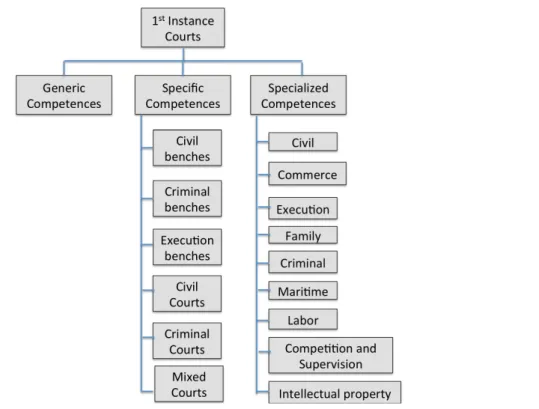
The Portuguese judicial system suffered recently (in 2014) a re-estructuration. The data used in this study (from 2010 to 2012) is prior to that re-estructuration. Before 2014 courts could be classified into various types: judicial courts, administrative and fiscal courts, the constitutional court, accounting court, military courts, and justice of peace courts (used to solve very small conflicts). The sample analysed in our empirical application corresponds to judicial courts, which develop their activity in the whole na-tional territory divided in ‘comarcas’ for the effect, which differ from the administrative distribution of the counties in Portugal (concelhos). Judicial courts divide in 3 instances: the 1st instance, which is the first level of decision, the 2nd instance, or Appeal courts, which is composed of relation courts and 3rd instance which corresponds to the Supreme Court of justice (which is the superior hierarchical body of the judicial courts). First instance judicial courts are organized within judicial districts, organized in circles, which are organized in judicial counties (comarcas), organized in smaller units - benches (consti-tuted mainly by a single judge and some administrative staff). Courts or Benches can be generic (addressing a large variety of cases), specific (addressing only certain processual forms) and specialized (where judges specialize in certain branches of law, like family, work, etc). Figure 1 illustrates how first instance courts are subdivided.
The 2014 reform (see Law 62/2013 regulated by Decree law, 49/2014) had two main purposes:, to implement specialized jurisdictions at the national level and to implement a new model of management of judicial counties. As a result of the reform, most generic courts and benches disappeared and work was centralized on specialized courts. Our analysis focus on generic competence benches (the most disaggregate unit of analysis). On the contrary Santos and Amado (2014) focused their analysis on the efficiency of judicial counties (Comarcas), analysing 223 of these during the period of 2007 to 2011. These judicial counties include generic competence and specialized courts that are not necessarily comparable.
Our sample comprises 267 benches of generic competence. Most of these benches are constituted by a single judge and they perform similar activities, being therefore
compa-!"#$%&"#'&()$ *+,-#"$ .)&)-/($ *+01)#)&()"$ 21)(/3($ *+01)#)&()"$ 21)(/'4/5)6$ *+01)#)&()"$ */7/4$ 8)&(9)"$ *-/0/&'4$ 8)&(9)"$ :;)(,<+&$ 8)&(9)"$ */7/4$ *+00)-()$ :;)(,<+&$ *-/0/&'4$ ='-/<0)$ >'0/4?$ @'8+-$ *+01)<<+&$'&6$ 2,1)-7/"/+&$ %&#)44)(#,'4$1-+1)-#?$ */7/4$ *+,-#"$ *-/0/&'4$ *+,-#"$ =/;)6$ *+,-#"$
Figure 1: Structure of Portuguese Judicial System
rable. We used data from 2010 to 2012 but these data were averaged and a single period analysis was performed (similarly to Schneider (2005)). The reasons for this averaging process relies on the picks of cases that some benches may have in some years due to mega-cases that consume most of the resources of a bench. Following the literature we chose as inputs the number of administrative workers (judges were not considered as most benches have a single judge), and average number of cases entered. Pending cases were not considered as they were not available. As a result, the input set does not reflect the entire workload of the court but it reflects the demand for courts’ services in a given pe-riod, and the ability of the court to satisfy that demand. The comparison between supply (cases resolved) and demand (incoming cases) leads to what is usually knows as clearance rate. Only when clearance rates are higher than 100% courts are able to catch up with backlog cases. Outputs considered in the assessments undertook are the average number of cases resolved in the period under analysis. In order to reflect the mix of caseload of benches, cases were partitioned into 6 categories, from an initial number of 27 types of cases identified as part of the work of the benches (see e.g. Kittelsen (1992) who used a
similar approach). The construction of the 6 categories took into account the similarity of competences required to solve the cases, such that each category was constituted by cases that followed a similar process. The final 6 categories are the following: 1- Common cases, provisional orders , embargoes and divorces (Common) 2 - Special cases, inven-tories,credit claims and workplace accidents (Special); 3- Civil enforcement and service judicial notice (Enforcement) 4 Corporate reorganization/bankruptcy (Bankruptcy) 5 -Guardianship cases (-Guardianship); 6- Other cases(Other)
For each of these six categories the number of cases entered was considered an input. In addition to these 6 inputs we also considered the input ’number of administrative workers’ in the court. The number of judges was not included in the input set as benches are divisions of a court represented by a single judge. As a result our court assessment in fact compares the performance of judges in handling the cases that were assigned to them.
This set of inputs and outputs raised the question that is addressed in this paper: What possible ways can be used to reflect the intrinsic link that exists between each input and each output? That is, the number of cases regarding e.g. civil enforcement that were resolved by the court is mainly linked with the number of cases of this type that the court received and not (directly) with the other types of incoming cases. Indirectly there could be a link, but this link is reflected in the global case load and case mix of the court (Some courts may receive more process of a certain type and therefore devoting less time to processes of the other types). The next section will describe the models put forth to resolve the problem of the intrinsic links between the inputs and the outputs in our courts example. Note however, that this problem is likely to appear in other settings too as discussed in the introduction.
Descriptive statistics for the input/output variables in, Table 1, show that on average the number of cases of various types entering the courts (-E) are higher than the number of cases resolved (-F), meaning that indeed backlog is accumulating in Portuguese general competence courts. Average clearance rates (CR), also shown, are generally very close to 100% or even below it, except in the case of bankruptcy cases where clearance rates (CR) are on average above 1 (1.14). Note however, that this type of cases are the ones with a lower value in Table 1 meaning that only a small percentage of the workload of a court is composed of these cases.
Average St DEv Max Min Av. CR Max CR Min CR Workers 6.84 2.55 12.3 1 Common-E 213.92 103.51 467.33 28 Special-E 91.99 55.09 264 0 Enforcement-E 340.20 194.07 1217.33 33.33 Bankruptcy-E 9.13 11.20 44.33 0 Guardianship-E 20.15 17.91 98.33 0 Others-E 27.34 23.16 103.67 0 Common-F 223.22 108.83 593 27 1.05 1.37 0.8 Special-F 87.40 50.09 237 0 0.98 2.43 0.48 Enforcement-F 236.74 128.91 672 14 0.72 2.58 0.17 Bankruptcy-F 9.11 10.58 44.33 0 1.14 6 0.21 Guardianship-F 20.25 17.54 85.67 0 1.05 2 0.50 Others-F 23.47 20.53 117 0 1.01 5.36 0.21
Table 1: Descriptive statistics
4
Output specific inputs - Alternative approaches
An output oriented directional distance function (see e.g. Chung et al. (1997)) under constant returns to scale (benches analysed are single judged and therefore comparable in size) will be used as a basis for efficiency computations. Generically we consider
a production technology with n DMUs, consuming m inputs (xij, i = 1, ..., m) and
producing s outputs (yrj, r = 1, ..., s). The directional vector (gyr, gxi) specifies the direction for improvement, but in our case we set gxi to zero. The directional distance model, for DMU o, is given by (1).
max λj,β n β| n X j=1 λjyrj ≥ yro+ βgyr, r = 1, . . . , s, (1) n X j=1 λjxij ≤ xio, i = 1, . . . , m, λj ≥ 0 ∀j o
The multiplier directional distance model, the dual of (1), is given by (2).
min ur,vi n ho = m X i=1 vixio− s X r=1 uryro | (2) − s X r=1 uryrj + m X i=1 vixij ≥ 0, j = 1, . . . , n, s X r=1 urgyr = 1, ur, vi ≥ 0 ∀r, ∀i o
Three approaches are going to be compared as a way of dealing with the output specific inputs in our courts example. The first approach will be called ‘Separation’ approach and corresponds to the analysis of the production process of each output separately and independently from the others. The second approach will be called the ‘Ratio’ approach and will replace outputs by clearance rates (the ratio between the cases resolved and the cases entered) for each type of case. The third approach will be called ‘Difference’ approach and will replace outputs by the difference between cases resolved and cases entered. Such a difference actually corresponds to the variation in the pending cases (i.e. when difference is positive pending cases reduced, when difference is negative the pending cases increased by the amount of the difference). In the next sections each of the approaches will be detailed and results obtained for each will be shown. Note that a distinctive feature between the three approaches lies on the assumptions regarding the production technology. The separation approach assumes that the production of each output can be modeled through an individual production process, while the other approaches assume that there is a single production process for the production of all outputs, and linkages between inputs and outputs are modeled through manipulation of the variables rather than changing the production possibility set.
Models (1) and (2), were the base model in all the approaches. A directional vector equal to unity was chosen in all cases. Such a vector implies that the resulting inefficiency scores are units dependent and not comparable across approaches given the different units of measurement of the variables. In order to compare the approaches we used the above models as a means to determine efficient output targets in terms of cases finished of each type r (CFr∗). After that a measure of efficiency was constructed for each output as CFr/CFr∗, where CFr stands for observed cases finished or resolved. After
obtaining these measures of output efficiency, they can be aggregated to generate an overall efficiency score. The way this aggregation is performed is not without implications. In the spirit of models 1 and 2, the maximum value obtained for each output should be regarded as the efficiency score (from these models we get, for a unitary directional vector, β ≤
Pn
j=1λjyrj
yro , r = 1, ..., m, meaning that the optimal value of β will be equal to the minimum ratio between target output and observed output, which is the same as to say that β equals the maximum ratio between the observed and target output). However, this maximum can hide important discrepancies between output efficiencies.
Averages could be used to resolve this problem and provide balanced overall efficiency scores. The average, cannot however, be used as it suffers from ‘aggregation inconsistency’ (see e.g F¨are and Karagiannis., 2014). In order to assure aggregation consistency in the final efficiency score computed we used a weighted average of the individual efficiency scores, where weights are the proportion of the target output in the total target output (CFr∗/Ps
r=1CF ∗
r). When this aggregation weight is used, the resulting overall aggregate
score is equal to the total of cases resolved divided by the total target cases resolved (Ps r=1CFr/ Ps r=1CF ∗ r).
4.1
Separation Approach
The separation approach assumes separable production functions for each output as first introduced in Banker (1992). A complete separation model would imply that the specific links between inputs and outputs are dealt with by computing the efficiency of output production in 6 distinctive models, one for each output. Clearly a single model can be solved for assessing the production of each output r, by considering different intensity variables for each output production process λr
j. The resulting model is shown in (3),
where xij is now replaced by xrj, since for each output r there is a corresponding input
i and therefore the same index is used, and Wj is the notation used for the joint input,
number of workers. max λr j,βr nXs r=1 βr| n X j=1 λrjyrj ≥ yro+ βrgyr, r = 1, . . . , s, (3) n X j=1 λrjxrj ≤ xro, r = 1, . . . , s, (4) n X j=1 λrjWj ≤ Wo, r = 1, . . . , s λj ≥ 0 o
This model is similar to that proposed by Cherchye et al. (2013) called also the decentralized efficiency score in Cherchye et al. (2015a), but we consider that the convexity
assumption holds for outputs. Note that we also considered an expansion factor βr
associated to each output to allow for as little dependence across the six categories of outputs as possible, and also because of technological sets having zero cases entered and zero cases finished, which created problems when a single expansion factor for outputs was adopted. The above model, replicates for each output production possibilities set the
constraint regarding the joint input. We modify the above model to take into account the fact that the workers are shared among the output production processes, and as a result a single constraint for workers could be used to replace the last constraint, assuming that a proportion αr of workers is used for the production of each output r :
Pn
j=1λ 1
jα1Wj+Pnj=1λ2jα2Wj+ ... +Pnj=1λ6jα6Wj ≤ Wo. This constraint is in the spirit
of Tsai and Molinero (2002), where a single constraint was used to model joint inputs in teaching and research in an university example, as pioneered by Beasley (1995) in a assessment of university departments. Note that similar models have been proposed by Cook and Hababou (2001) in the context of assessing service and sales performance in bank branches, where some inputs and outputs were specific to each of these functions but some inputs were shared by both. Both Tsai and Molinero (2002) and Beasley (1995) have let the model determine the optimal shares of joint resource allocated to each process. In our case, there is no observed allocation of the joint input over each output, and as a result leaving the model to ’choose’ this allocation, when there is no observed allocation seemed a rather arbitrary procedure. We therefore set αr equal to (m1). Note that the
objective of using this share is to turn the scale of the left hand side and right hand
side comparable. An alternative approach would be to multiply Wo on the right hand
side by 6, since on the left hand side this variable is being considered 6 times - one for each process specific technology. As a result, any other definition of the share would be arbitrary (and in fact would not work as several attempts revealed).
As a result the separation approach model that we applied to the courts example is shown in (5). max λr j,βr nXs r=1 βr| n X j=1 λrjyrj ≥ yro+ βrgyr, r = 1, . . . , s, (5) n X j=1 λrjxrj ≤ xro, r = 1, . . . , s, (6) s X r=1 n X j=1 λrjαrWj ≤ Wo, λj ≥ 0 o
Applying model (5) to the Courts data, with a unitary directional vector, resulted in the outputs efficiency scores shown in Table 2.
Common Special Enforcement Bankruptcy Guardianship Others Score 78.12% 69.48% 28.54% 90.31% 86.14% 42.97%
Table 2: Results for each output efficiency using separation approach
The output showing the highest efficiency is bankruptcy cases, meaning that courts in general resolve a high number of these cases given the resources available and the cases received (note that in absolute terms this is the lowest volume input - see Table 1 - and the one with the highest clearance rate). The output with least efficiency is ‘enforcement cases’, where courts resolve on average a low number of such cases given the workforce and the number of cases of this type the court received (in absolute terms this is the type of cases with higher volume and lower clearance rates). In terms of aggregate efficiency the mean for the total sample of courts is 44.33%. No court is considered 100% efficient, meaning that none showed maximum efficiency in the production of all outputs.
4.2
Ratio Approach
The second approach that we consider for dealing with output-specific inputs is based on the fact that the ratios between the outputs and the output-specific inputs entail a meaning: clearance rates, used commonly as a KPI in assessing the performance of courts. Courts with a clearance rate above 1 are clearing pending cases, as they resolve more cases than the ones that entered the court. On the contrary clearance rates below 1 mean that pending cases are accumulating. The use of ratios to reflect direct linkages between volume inputs and outputs can be seen as the opposite approach to that taken in Thanassoulis et al. (1995), where ratios were replaced by volume measures. The replace-ment of volume measures by ratios has been suggested before, although not necessarily with the purpose addressed in this paper. For example, Despic et al. (2007) propose solv-ing DEA models through a replacement of all variables in the model by all possible ratios between outputs and inputs. Ratios are considered then the outputs of a DEA model with a single unitary input. Results from this modified model and the traditional DEA model are not coincident, but are somehow related, as shown by Despic et al. (2007). Clearly, only the ratios that correspond to links of interest between inputs and outputs may be considered under this approach, and as a result the linkages can be reflected in the chosen ratios. In our case we did not follow this approach given the existence of the joint input relating to number of workers. As we were interested in using the model to determine targets we would face a problem as we would have for each output (e.g. num-ber of common cases solved) two targets: One for the ratio between ‘N. Common cases
resolved’/‘Workers’ and another for the ratio ‘N. Common cases resolved’/‘N. Common cases entered’. As a result, we decided to keep on the input side the number of workers and using the clearance rates on the output side. This raised another problem. That of mixing a volume measure with ratio data, which by definition are adimensional. The implications of permitting this mix of variable types would be that smaller courts, with a low number of workers, but reasonable clearance rates would become efficient. Under a CRS model this would imply unachievable and unrealistic targets for most units.
The problems arising from mixing ratio data with volume measures are relatively well known and have been addressed before (e.g. Hollingsworth and Smith (2003) or Emrouznejad and Amin (2009)). There are two known problems related to DEA models applied to ratio data: (1) the violation of the proportionality implicit in constant returns to scale (this violation is not a problem under variable returns to scale), and (2) the convexity problem analysed in Emrouznejad and Amin (2009), where convex targets formed from ratios may lie on the interior or outside of the production possibility set formed by volume measures. This happens because a convex combination of ratios is not equivalent to the ratio between the convex combination of the respective numerators and denominators. Recently Olesen et al. (2015) addressed extensively the issue of ratio and volume variables in DEA models and proposed models that can address the above problems. An interesting remark made by the authors is that not all ratios are the same. As a result, ratios are classified into: proportional ratios (those that increase proportionality with the increase in volume measures), fixed ratios (those that do not vary when volume measures change), downward proportional ratios (are proportional when volume measures decrease but fixed when they increase), and upward proportional ratios (are proportional when volume measures increase, but fixed when volume measures decrease). Our ratio measures (clearance rates) may be considered fixed ratios. That is, when the number of workers increases it is expected that the number of cases entered and number of cases resolved also increase by a similar proportion. However, as a single judge is dealing with the cases very large increases in the number of workers will not translate in proportional increases in cases.
Considering the ratios in our illustrative example fixed, the proportionality and con-vexity problems are solved adapting the linear model proposed by Olesen et al. (2015) where the volume input responds to scale and the ratio outputs are fixed. This model
with only fixed ratios (Rrj) and a single input measure (Wj) is shown in (7) adapted to
the case of a directional output distance function.
max λj,β,αj n β| n X j=1 λjαjWj ≤ Wo, λj(Rrj − (Rro+ βgRr)) ≥ 0, r = 1, . . . , s, j = 1, ..., n n X j=1 λj = 1, λj ≥ 0 ∀j o (7) The first constraint allows for proportionality on the volume input through αj, whereas
λj is restricted to sum 1. The second set of constraints assure that only when the ratio
r of the peer unit j is greater than the ratio for the observed unit (Rro), the intensity
variable for peer j (λj) can be greater than zero. Model (7) is not, however, interesting
as αj equal to zero always satisfies the first constraint. The first solution to solve this
problem is to ignore the scaling of inputs and treat the model as VRS. This would result in fact in a FDH model as shown in Podinovski (2005). The second solution would be to add volume outputs (yrj) to the above model and allow the scaling of inputs by α
and the scaling of volume outputs by the same proportion. This second alternative was adopted given the knowledge we have about the numerators and denominators of the ratio measures, and is shown in model (8) (the first alternative should be preferred if this knowledge did not exist).
max λj,β,αjkj n β| n X j=1 λjαjWj ≤ Wo, (8) (Rro+ βgRr) − Rrj ≤ M (1 − kj), r = 1, . . . , s, j = 1, ..., n, λj ≤ kj, j = 1, ...n n X j=1 λjαjyrj ≥ yro, r = 1, . . . , s n X j=1 λj = 1, λj ≥ 0, kj ∈ {0, 1} ∀j o
Solving model (8) involved replacing the product αjλj by a new variable, such that
the non-linearity of the constraints was removed. Note that given the knowledge about the numerator and denominator the approach of Emrouznejad and Amin (2009) could be used to replace the second set of constraints by
Pn
j=1λjyrj
Pn
j=1λjxrj ≥ Rro+ βgRr. This approach was not followed in order to allow for its flexibility when dealing with cases where only ratios are known.
Targets from model (8) are obtained directly form the ratio targets: R∗rj, which can be converted to the target finished cases that the court in question should attain (CFrj∗ =
Rrj∗ × cases type r entered), when it is compared to other courts with higher clearance rates and simultaneously lower number of workers.
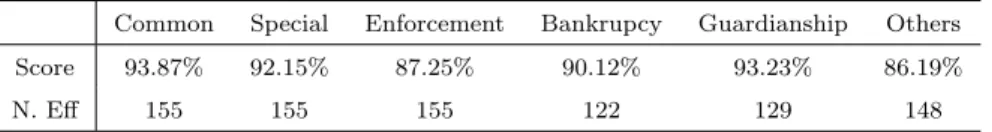
Results from applying the ratio model (8) to our sample of courts revealed an average aggregate efficiency of 90.11% with 155 courts appearing with 100% efficiency. In terms of average output efficiencies these are displayed in Table 3 together with the number of courts showing 100% efficiency in the production of each output.
Common Special Enforcement Bankrupcy Guardianship Others Score 93.87% 92.15% 87.25% 90.12% 93.23% 86.19%
N. Eff 155 155 155 122 129 148
Table 3: Results for each output efficiency using ratio approach
Common cases are those where courts reveal higher efficiency, this is followed by guardianship and special cases. The output whose production is less efficient is the other cases.
4.3
Difference Approach
The third and last approach that we consider for dealing with output-specific inputs is based on the fact that the differences between the outputs and the input-specific outputs entail a meaning related to pending cases: pending cases at the end of a particular period are equal to: pending cases at the beginning of the period, plus incoming cases of the period minus cases resolved during the period. As a result the difference between resolved cases and new cases entered (our outputs and inputs) yields the variation in pending cases (i.e. initial number of pending cases minus the pending cases in the end of the period). A positive value in the difference means that there was an effective reduction in pending cases as the pending cases in the end of the period are lower to those at the beginning. When the difference is negative, it means that pending cases built up.
Taking differences between outputs and output-specific inputs is equivalent to the consideration of weight restrictions where one imposes the weights on inputs and corre-sponding outputs to be the same. Weight restrictions that link inputs and outputs are called ARII constraints (see Thompson et al. (1990, 1992)). Note that the weights deter-mined in a DEA model are units dependent meaning that the equality between weights can be done directly when the unit of measurement is the same, or should take the units of measurement into account when that is not the case.
Model (1) added of these weight restrictions (WR), is shown in (9), for our specific setting of 6 inputs (x1, ..., x6) linked to the production of 6 outputs (y1, ..., y6), and one
joint input (W1, ..., W6). min ur,vi,v n ho = − 6 X r=1 ur yro+ 6 X i=1 vi xio + vWo| (9) − 6 X r=1 ur yrj+ 6 X i=1 vi xij + v Wj ≥ 0, j = 1, . . . , n, 6 X r=1 ur gyr = 1, u1 = v1, u2 = v2, u3 = v3, u4 = v4, u5 = v5, u6 = v6, u ≥ 0, v ≥ 0 o
Setting u1 = v1 = w1 and u2 = v2 = w2, etc. results in the equivalent model (10):
min wr,v n ho = − 6 X r=1 wr(yro− xro) + vWo | (10) − 6 X r=1 wr(yrj− xrj) + vWj ≥ 0, j = 1, . . . , n, 6 X r=1 wr gyr = 1, w ≥ 0 o
The dual is shown in (11).
max λj,β n β | n X j=1 λj (yrj − xrj) ≥ (yro− xro) + βgyr, r = 1, ..., 6 (11) n X j=1 λj Wj ≤ Wo, λj ≥ 0 o
The dual model in (11) has 6 output constraints and one input constraint - if no joint inputs had been considered we would end up with a model with just outputs and no inputs, that is infeasible (multiplier) or unbounded (envelopment). In the presence of joint inputs this problem does not arise. In the absence of joint inputs one way to solve the infeasibility problem would be to consider a unitary input. This, however would change returns to scale assumptions.
Running model (11) or (10) using a unitary directional vector yields the results shown in Table 4 for each output average efficiency. Overall 15 units have been identified as 100% efficient and the aggregate efficiency was 85.84%.
Common Special Enforcement Bankrupcy Guardianship Others Score 93.75% 87.69% 81.63% 64.07% 82.48% 70.98
N. Eff 15 15 15 11 14 14
Table 4: Results for each output efficiency using difference approach
Common cases are again those where courts reveal higher efficiency, this is followed by special cases and then by guardianship. The output whose production is less efficient is bankruptcy cases, (contrarily to the other approaches that identified bankruptcy cases as the ones with higher efficiency), followed by other cases (consistently with the other two approaches).
5
Comparing Approaches
Efficiency values obtained from the various approaches can be compared because they have been computed based on target finish cases from each approach. Higher efficiency values, mean therefore targets that are closer to observed values - less demanding.
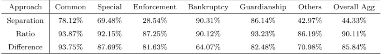
The average efficiencies obtained from the 3 approaches in the production of the 6 outputs are shown in Table 5.
Approach Common Special Enforcement Bankruptcy Guardianship Others Overall Agg Separation 78.12% 69.48% 28.54% 90.31% 86.14% 42.97% 44.33%
Ratio 93.87% 92.15% 87.25% 90.12% 93.23% 86.19% 90.11% Difference 93.75% 87.69% 81.63% 64.07% 82.48% 70.98% 85.84%
Table 5: Results for each output efficiency and overall efficiency in three approaches Higher efficiency scores mean targets that are closer to observed values and lower efficiency scores mean more demanding targets. As a result, the ratio approach is the one yielding closer targets to observed values in most cases. Aggregate overall efficiency is also the highest for the ratio approach. Regarding the ranking of output efficiencies, the ratio and separation approaches, consider that the cases where courts are most efficient are Common cases. The 3 approaches show different outputs as the least efficient: under the separation approach the least efficiency of courts is in dealing with enforcement cases, other cases are identified as the least efficient by the ratio approach and bankruptcy are identified by the differences approach.
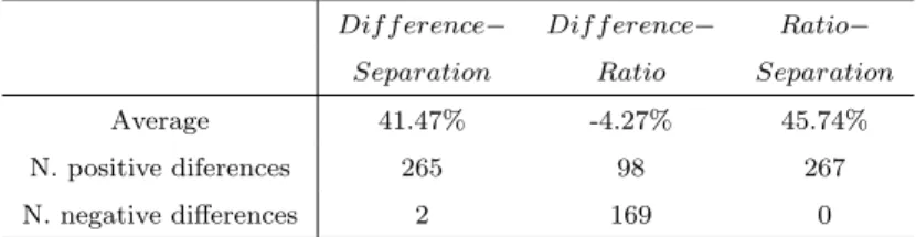
be-between the separation and the ratio approach (0.46). The highest correlation is be-between the separation and the difference (0.61). The correlation between ranks follows a similar pattern and the magnitude of the coefficients is very similar, with the highest correlation happening between the separation and difference approaches (close to 0.8). Computing differences between the aggregate efficiencies of the various methods results in the values shown in Table 6.
Dif f erence− Dif f erence− Ratio− Separation Ratio Separation Average 41.47% -4.27% 45.74% N. positive diferences 265 98 267 N. negative differences 2 169 0
Table 6: Differences between scores of the 3 approaches
The above results show that the ratio approach has produced always higher or equal (the zero is contained in the positive differences in Table 6) aggregate scores than the separation approach. The difference approach in the majority of cases also has higher efficiency scores than the separation approach, but in this case two benches are exceptions to this rule. On average the separation approach is about 40 percentage points below the ratio and the difference approaches in terms of aggregate efficiency. As a result the difference and ratio approaches are the closest in terms of efficiency scores. Note however that in terms of rank correlation the highest similarities are between the separation and difference approaches.
Our aim in this paper is not to compare mathematically the 3 approaches, since they use different assumptions and variables. However, the above results are intuitively expected. The separation approach is clearly the one where lower efficiency scores are to be obtained, due to the fact that each output is optimized in an output specific production set. On the contrary, the ratio approach is the one where higher efficiency scores are expected because by definition ratios do not verify the convexity assumption and as a result a non-convex model (of the FDH type) is clearly less discriminating and results in a higher number of frontier units. Note that one may be inclined to think that the higher number of efficient units in this case is due to different returns to scale assumption used in the ratio model and the remaining models. We attribute higher efficiency scores to the non-convex assumptions on ratios, but not on returns to scale assumptions. Since ratios are adimensional measures whose comparison and computation always ignores issues of
scale, in the presence of ratio data, no other assumption for these variables can be invoked than constant returns to scale.
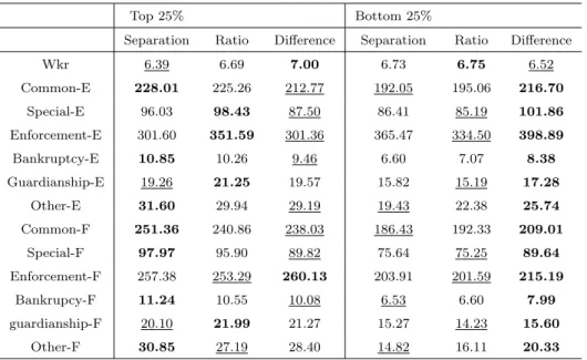
A more detailed analysis was performed regarding the characteristics of the best and worst performers under all approaches. For that purpose we divided the sample into the top 25% performers (as the 67 units with highest efficiency) and the bottom 25% performers (as the 67 units with lowest efficiency), and computed the average inputs and outputs for each of these groups. Results are shown in Table 7.
Top 25% Bottom 25%
Separation Ratio Difference Separation Ratio Difference
Wkr 6.39 6.69 7.00 6.73 6.75 6.52 Common-E 228.01 225.26 212.77 192.05 195.06 216.70 Special-E 96.03 98.43 87.50 86.41 85.19 101.86 Enforcement-E 301.60 351.59 301.36 365.47 334.50 398.89 Bankruptcy-E 10.85 10.26 9.46 6.60 7.07 8.38 Guardianship-E 19.26 21.25 19.57 15.82 15.19 17.28 Other-E 31.60 29.94 29.19 19.43 22.38 25.74 Common-F 251.36 240.86 238.03 186.43 192.33 209.01 Special-F 97.97 95.90 89.82 75.64 75.25 89.64 Enforcement-F 257.38 253.29 260.13 203.91 201.59 215.19 Bankrupcy-F 11.24 10.55 10.08 6.53 6.60 7.99 guardianship-F 20.10 21.99 21.27 15.27 14.23 15.60 Other-F 30.85 27.19 28.40 14.82 16.11 20.33
Table 7: Characteristics of best and worst performers in the 3 approaches
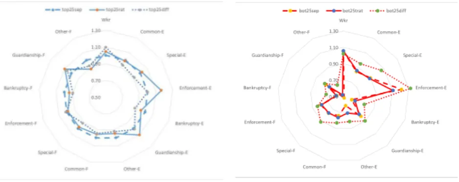
In bold we signal the highest average values and we use under script to signal the lowest. In spite of the different efficiency scores obtained under each approach, there is consistency on the characteristics of the best and worst performing units under each approach. This can be seen in Figure 2 where we use as a basis the top performers under the separation approach and compare the average performance of the various groups in relation to this one.
The graph on the left shows that best performers are similar between approaches, with the ratio approach identifying top performers with slightly more inputs than the top performers of the other approaches and similar or lower outputs (revealing that under the ratio approach top performers appear on average the least efficient. The graph on the right compares worst performers between approaches, where it is clear that the bottom performers identified in the differences approach are on average dealing with more cases than the worst performers in the other two approaches (where the worst performers are
!"#! !"$! !"%! &"&! &"'! ()* +,--,./0 1234567/0 0.8,*43-3.9/0 :6.)*;294</0 =;6*>56.?@52/0 A9@3*/0 +,--,./B 1234567/B 0.8,*43-3.9/B :6.)*;294</B =;6*>56.?@52/B A9@3*/B C,9D#?32 C,9D#9*69 C,9D#>588
Figure 2: Characteristics of top performers and bottom performers under each approach
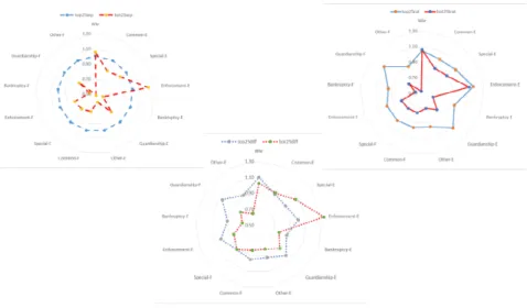
Comparing now best and worst performers within approaches (see Figure 3) we can see that under the ratio and separation approaches best performers generally deal with more cases than worst performers, they have in general more cases in and more cases out. For the differences approach worst performers show particularly high enforcement cases entering the court, and similar or higher number of cases for the remaining types of processes, but they show lower cases finished than the best performers.
Analysing specifically the cases that showed the highest differences in ranking between approaches we show in Table 8 the observed values of the volume measures, the clearance ratios, and the differences between finished cases and entered cases for these units. We also show the total average of the sample as a means of comparison.
Figure 3: Characteristics of top performers and bottom performers within each approach Eff Separation 0.3352 0.6769 0.3242 0.4361 Eff Ratio 1 1 1 0.7702 Eff Diff 0.7291 0.679 0.6303 0.9401 T24 T261 T68 T95 Average Sample Wkr 8.5 2 4 6 6.84 Common-E 251.33 402.67 116 118.33 213.92 Special-E 105.67 184 52.33 64 91.99 Enforcement-E 536.67 644.67 283.67 172.67 340.20 Bankruptcy-E 2.67 19.33 4 9.12 Guardianship-E 43.67 33.17 17.33 20.15 Other-E 2 62.33 3.33 2.67 27.341 Common-F 213.33 394.67 102.67 133 223.22 Special-F 101.67 152.33 46.33 56 87.40 Enforcement-F 285 272 137 125.67 236.74 Bankruptcy-F 3.33 16.33 2 9.11 Guardianship-F 49 30.33 20.33 20.25 Other-F 1.33 51.67 8 2.33 23.46 Clearance rates Common 0.85 0.98 0.89 1.12 1.05 Special 0.96 0.83 0.89 0.88 0.98 Enforcement 0.53 0.42 0.48 0.73 0.723 Bankruptcy 1.25 0.84 0.50 1.14 Guardianship 1.12 0.91 1.17 1.05 Other 0.67 0.83 2.40 0.88 1.01 Differences Common -38 -8 -13.33 14.67 9.31 Special -4 -31.67 -6 -8 -4.59 Enforcement -251.67 -372.67 -146.67 -47 -103.46 Bankruptcy 0.67 -3 -2 -0.016
Table 8: Characteristics of some units with large differences in ranking between ap-proaches
Benches T24 and T68 are top performers under the ratio approach and bottom per-formers under the separation and differences approaches. T24 and T68 are efficient under the ratio approach because they excel in at least one of the clearance rates. Bench T68 shows one outstanding clearance rate (of 2.4 for other cases) and simultaneously a small number of workers, which makes it comparatively better than its peers. bench T24 shows a good performance performance in the clearance rate of bankruptcy and guardianship cases, in spite of a clearly above average number of workers, making it also better than its peers. Note however, that the ratio model does not take into account the fact that the clearance rate of 2.4 for other cases of T68 does not represent a big amount of work as only about 3 cases of this type entered the court during the period of analysis. This high rate just meant the clearance of about 8 cases, which cannot be considered enough to compensate for the low performance of this bench in dealing with other cases. Both the separation approaches and the difference approach, working with volume measures, take this fact into account and attribute to this unit an efficiency score that places it among the bottom 25% units. Regarding bench T261 it is a top performer on the separation approach and ratio approach, but a bottom 25% performer in the difference approach. This is clearly a result of a very low number of workers of this court and a high level of outputs (above average in all the approaches) - this makes units neglect the number of cases entered when maximizing their efficiency score under the separation approach. As a result this unit appears very efficient, but the fact is that it finishes a lower number of cases than those that entered in the court for all types of cases, meaning that backlog is building up in this court. The inefficiency of this court may in fact be attributed to an insufficient number of workers for the cases received. This is not however technical ineffi-ciency, but allocative inefficiency. This means that the difference approach and the ratio approach by imposing strict links between inputs and outputs may indeed be capturing more than just technical efficiency. Regarding bench T95 this is a top performer under the difference approach, but a low performer under the ratio approach. This bench shows a good performance in clearance rates, when compared for example with T261, but much higher number of workers. Regarding the differences, indeed this is the bench in Table 8 showing a better balance in terms of the differences, in spite of the small values being
indicative of the small size of the bench.
As a summary from the above we tend to favor the use of differences or the separation approach as a way to link inputs and outputs that relate directly. The use of differences is equivalent to the use of weight restrictions that impose equal weighting to the linked inputs and outputs. It may however be a less general approach in the sense that the computation of differences needs to yield a observable and meaningful measure (which in our case was a measure of reduction in backlog). In case the differences cannot be computed the separation approach appears as a very similar alternative, where rank correlations with the difference approach are close to 80% and the absolute differences in rankings is the lowest on average between these two approaches (it is 33 places difference on average as compared to 93 places average difference between the difference and the ratio approaches - the most dissimilar ones).
6
Conclusion & Discussion
This paper has addressed the topic of establishing links between specific inputs and outputs in efficiency assessments. This is a topic that has deserved recent attention in the literature, with some new developed models advocating the use of output specific production functions and thus separate efficiency assessments. Through an illustrative example on Portuguese courts’ efficiency we have compared separate assessments with two other approaches that could be used in establishing the links between inputs and outputs: One is the ratio approach, where output specific inputs are linked to outputs through a ratio, and the other is the differences approach, where linkages are established through differences. From this comparative study we conclude that the approach used to reflect the linkages between inputs and outputs is not indifferent in terms of results produced. The various approaches revealed some strengths and fragilities. Some of the fragilities arose from modelling options, particularly in the ratio case, where the impossibility of straightforwardly use ratio and volume measures in a standard DEA model generated a non-convex model, which lead to less discriminating results, not necessarily comparable with the remaining approaches. It is our view that the ratio model is not a particularly good option for linking inputs and outputs in spite of it being probably the most intuitive - particularly in the Court’s context where clearance rates are often used as a performance
measures. The main reason for this is related to the low discrimination between units that models suited to deal with this type of variables end up producing. In spite of that the characteristics of top performers in the ratio approach and bottom performers is not dramatically different from those resulting from the other two approaches. The separation approach, by treating each output independently from the rest ends up in very low efficiency scores and therefore demanding targets. However in terms of ranking and in terms of worst and best performers the separation and the difference approaches are in fact very similar, constituting two good alternatives for handling the type of linkages between inputs and outputs addressed in this paper. The analysis of Portuguese courts has been illustrative in this paper. In spite of that, there appears to be huge inefficiencies in courts in Portugal, with large discrepancies between the number of cases received and solved and the staff employed. Future work should pass through an in-depth analysis of these inefficiencies (particularly after the reform in 2014) and an investigation of how resources could be better re-allocated between courts. This could be a valuable input for the executive power, which could use this type of analysis to better allocate its scarce resources.
7
Acknowledgments
The author is grateful to Raquel Prata who collected and performed a first analysis of the data used in this study. This analysis is published in her Master thesis entitled “Contributo para a avalia¸c˜ao da eficiˆencia dos tribunais”, which is available at ISCTE Business School, Lisbon. The author also benefited from some comments and remarks received when discussing the paper with Victor Podinovski, Ole Olesen, Veerle Hennebel and Laurens Cherchye. All contents are the sole responsibility of the author.
References
Banker, R. (1992). Selection of efficiency evaluation models. Contemporary Accounting Research, 9(1):343–355.
Beasley, J. (1995). Determining teaching and research efficiencies. Journal of the Opera-tional Research Society, 46:441–452.
Cherchye, L., De Rock, B., and Hennebel, V. (2015a). Coordination efficiency in multi-output settings:a dea approach. Annals of Operations Research, In press.
Cherchye, L., Rock, B. D., Dierynck, B., Roodhooft, F., and Sabbe, J. (2013). Opening the black box of efficiency measurement: Input allocation in multi-output settings. Operations Research, 61(5):1148 – 1165.
Cherchye, L., Rock, B. D., and Walheer, B. (2015b). Multi-output efficiency with good and bad outputs. European Journal of Operational Research, 240:872 – 881.
Chung, Y., F¨are, R., and Grosskopf, S. (1997). Productivity and undesirable outputs:
a directional distance function approach. Journal of Environmental Management,
51(3):229–240.
Cook, W. D. and Hababou, M. (2001). Sales performance measurement in bank branches. Omega, The International Journal of Management Science, 29:299–307.
Despic, O., Despic, M., and Paradi, J. (2007). DEA-R: ratio-based comparative effi-ciency model, its mathematical relation to DEA and its use in applications. Journal of Productivity Analysis, 28:33–44.
Deyneli, F. (2011). Analysis of relationship between efficiency of justice services and salaries of judges with two stage DEA method. European Journal of Law and Eco-nomics, 34(3):477–493.
Emrouznejad, A. and Amin, G. R. (2009). Dea models for ratio data: Convexity consid-eration. Applied Mathematical Modelling, 33(1):486–498.
Falavigna, G., Ippoliti, R., Manello, A., and Ramello., G. (2015). Judicial productivity, delay and efficiency: A directional distance function (ddf) approach. European Journal of Operational Research, 240:592 – 601.
F¨are, R. and Karagiannis., G. (2014). A postcript on aggregate farrell efficiencies. Euro-pean Journal of Operational Research, 233:784 – 786.
Gorman, M. F. and Ruggiero, J. (2009). Evaluating U.S. judicial district prosecutor performance using dea: are disadvantaged counties more inefficient? European Journal of Law and Economics, 27(3):275–283.
Hollingsworth, B. and Smith, P. (2003). Use of ratios in data envelopment analysis. Applied Economics Letters, 10:733–735.
Kittelsen, S. A. C.and Førsund, F. R. (1992). Efficiency analysis of Norwegian district courts. Journal of Productivity Analysis, 3(3):277 – 306.
Lewin, A. Y., Morey, R. C., and Cook, T. J. (1982). Evaluating the administrative effi-ciency of courts. Omega, The International Journal of Management Science, 10(4):401 – 411.
Olesen, O. B., Petersen, N. C., and Podinovski, V. V. (2015). Efficiency analysis with ratio measures. European Journal of Operational Research, 245:446–462.
Pedraja-Chaparro, F. and Salinas-Jimenez, J. (1996). An assessment of the efficiency of spanish courts using DEA. Applied Economics, 28(11):1391–1403.
Podinovski, V. (2005). Selective convexity in DEA models. European Journal of Opera-tional Research, 161:552 – 563.
Portela, M. and Camanho, A. (2010). Analysis of complementary methodologies for the estimation of school value-added. Journal of the Operational Research Society, 61:1122 – 1132.
Portela, M., Camanho, A., and Borges, D. (2012). Performance assessment of secondary schools: the snapshot of a country taken by dea. Journal of the Operational Research Society, 63:1098 – 1115.
Posner, R. (2000). Is the ninth circuit too large? a statistical study of judicial quality. The Journal of Legal Studies, 29(2):711–719.
Salerian, J. and Chan, C. (2005). Restricting multiple-output multiple-input DEA models by disagregating the output-input vector. Journal of Productivity Analysis, 24:5–29. Santos, S. and Amado, C. (2014). On the need for reform of the portuguese judicial system
- does data envelopment analysis assessment support it? Omega, The International
Journal of Management Science, 47:1 – 16.
Schneider, M. (2005). Judicial career incentives and court performance: An empirical study of the german labour courts of appeal. European Journal of Law and Economics, 20(2):127–144.
Thanassoulis, E., Boussofiane, A., and Dyson, R. G. (1995). Exploring output quality targets in the provision of perinatal care in England using data envelopment analysis. European Journal of Operational Research, 80:588–607.
Thompson, R., Langemeier, L., Lee, C., Lee, E., and Thrall, R. M. (1990). The role of multiplier boundas in efficiency analysis with application to kansas farming. Journal of Econometrics, 46:93–108.
Thompson, R. G., Lee, E., and Thrall, R. M. (1992). DEA/AR-efficiency of U.S. indepen-dent oil/gas producers over time. Computers and Operations Research, 19(5):377–391.
Tsai, P. and Molinero, C. M. (2002). A variable returns to scale data envelopment
analysis model for the joint determination of efficiencies with an example of the UK health service. European Journal of Operational Research, 141(1):2138.
Voigt, S. (2014). Determinants of judicial efficiency: A survey. Available at SSRN: http://ssrn.com/abstract=2390704 or http://dx.doi.org/10.2139/ssrn.2390704.