www.nat-hazards-earth-syst-sci.net/13/3405/2013/ doi:10.5194/nhess-13-3405-2013
© Author(s) 2013. CC Attribution 3.0 License.
Natural Hazards
and Earth System
Sciences
Impacts of groundwater extraction on salinization risk in a
semi-arid floodplain
S. Alaghmand1, S. Beecham1, and A. Hassanli1,2
1Centre for Water Management and Reuse, School of Natural and Built Environments, University of South Australia, Adelaide, Australia
2College of Agriculture, Shiraz University, Shiraz, Iran
Correspondence to:S. Alaghmand ([email protected])
Received: 24 April 2013 – Published in Nat. Hazards Earth Syst. Sci. Discuss.: 26 July 2013 Revised: 29 October 2013 – Accepted: 6 November 2013 – Published: 23 December 2013
Abstract.In the lower River Murray in Australia, a combina-tion of a reduccombina-tion in the frequency, duracombina-tion and magnitude of natural floods, rising saline water tables in floodplains, and excessive evapotranspiration have led to an irrigation-induced groundwater mound forcing the naturally saline groundwater onto the floodplain. It is during the attenua-tion phase of floods that these large salt accumulaattenua-tions are likely to be mobilised and discharged into the river. This has been highlighted as the most significant risk in the Murray– Darling Basin and the South Australian Government and catchment management authorities have subsequently de-veloped salt interception schemes (SIS). The aim of these schemes is to reduce the hydraulic gradient that drives the regional saline groundwater towards the River Murray. This paper investigates the interactions between a river (River Murray in South Australia) and a saline semi-arid flood-plain (Clark’s floodflood-plain) that is significantly influenced by groundwater lowering due to a particular SIS. The results confirm that groundwater extraction maintains a lower wa-ter table and a higher amount of fresh river wawa-ter flux to the saline floodplain aquifer. In terms of salinity, this may lead to less solute stored in the floodplain aquifer. This occurs through three mechanisms, namely extraction of the solute mass from the system, reducing the saline groundwater flux from the highland to the floodplain and changing the flood-plain groundwater regime from a losing to a gaining one. It is shown that groundwater extraction is able to remove some of the solute stored in the unsaturated zone and this can mit-igate the floodplain salinity risk. A conceptual model of the impact of groundwater extraction on floodplain salinization has been developed.
1 Introduction
Figure 2 Configuration of SIS produ tion ells in lue and o ser ation ells in red at the Clark’s Floodplain. The inset
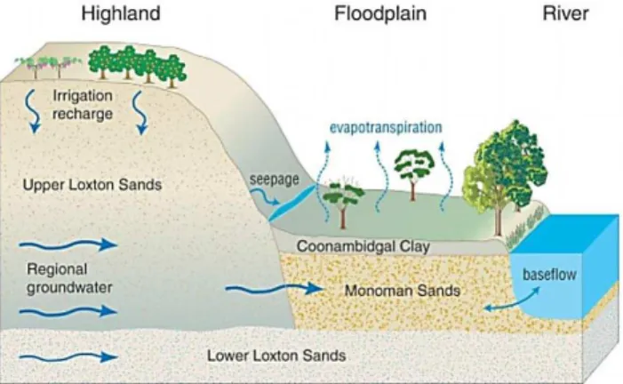
Fig. 1.Conceptual model of groundwater inputs to the floodplain and potential groundwater discharge pathways within the floodplain in the lower River Murray (Holland et al., 2009a).
water resulted in rising water table levels and the formation of a large groundwater mound during the wet season of 2000 (Petheram et al., 2008).
Prior to 2010, a high river flood event had not occurred for 13 yr. However, salt accumulation had continued over this period. The Independent Audit Group for Salinity (IAG-Salinity) mentioned the likelihood of severe salt accessions during flood recessions in their report (MDBA, 2010). This was articulated in their 1st recommendation and in the pre-vious audit reports. IAG-Salinity considers this the most sig-nificant risk in the Murray–Darling Basin. As an effort to reduce the immediate risk of river salt accession induced by increased saline groundwater levels, due to field irriga-tion and excessive evaporairriga-tion, the South Australian Gov-ernment and catchment management authorities have devel-oped salt interception schemes to pump the highly saline groundwater mixed with irrigation recharge from the flood-plain to evaporation basins (DWR, 2001). Each bore yields 2–3 L s−1 to reduce the hydraulic gradient that drives the regional saline groundwater towards the River Murray and this has improved river water quality (Berens et al., 2009). The SIS bores have been in operation since August 2005 except for some periods of shut down (e.g. from Novem-ber 2006 to May 2007). It is expected they will prevent about 200 tonnes of salt per day from entering the River Murray by 2040 (White et al., 2009). Before the SISs were opera-tional, an irrigation-induced groundwater mound forcing the naturally saline groundwater onto the floodplain at a rela-tively high flow rate, thereby increasing soil salinity in the root zone of the floodplain woodlands (Viezzoli et al., 2009; Doble, 2004) (Fig. 1). For instance at Clark’s floodplain, field investigations have shown that significant salt accumulation and vegetation dieback has occurred. This is due to evapo-transpiration from rising floodplain water tables, altered flow regimes and increased irrigation in the surrounding highlands on this floodplain (Doble, 2004).
Some of the most challenging aspects of water resources studies concern the interaction between surface and ground-water (Wheater et al., 2010). Rassam (2011) classified flow and solute exchange between a river and a floodplain aquifer into four categories: (1) natural exchange flux due to river stage fluctuations such as flooding (within-bank or over-bank), base-flow discharge, reservoir regulations, etc. (Squil-lace, 1996; Chen, 2003; Moench and Barlow, 2000; Brut-saert and Lopez, 1998); (2) exchange flux induced by pump-ing wells in adjacent aquifers (Chen and Shu, 2006; Sopho-cleous et al., 1995; Sun and Zhan, 2007); (3) exchange flux due to changes in recharge rates; and (4) exchange flux due to changes in evapotranspiration. Groundwater extraction is an important process that affects the exchange flux between surface water and groundwater. Extraction-induced river de-pletion is defined as the reduction of river flow due to induced infiltration of stream water into the aquifer or the capture of aquifer discharge to the river (Rassam, 2011). The temporal and spatial scales at which these processes contribute to the exchange flux is variable. For instance, river depletion result-ing from groundwater extraction is delayed by time lags that range from days to hundreds of years. Likewise, the extent of the groundwater extraction activity may vary along a river reach, thus leading to gaining and losing sub-reaches. Be-cause of the intensive spatial and temporal variability there is a need for dynamic modelling of their impacts on river flows.
Figure 2 Configuration of SIS produ tion ells in lue and o ser ation ells in red at the Clark’s Floodplain. The inset
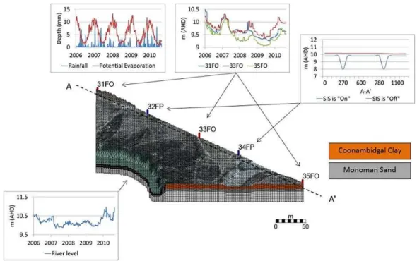
Fig. 2.Configuration of SIS production wells (in blue) and observation wells (in red) at Clark’s floodplain. The inset map shows the location of the Bookpurnong floodplain in Australia.
2007). Modelling of surface–groundwater interactions needs knowledge of groundwater modelling, but also a detailed un-derstanding of the exchange processes that occur between the surface and sub-surface domains (Barnett et al., 2012). Surface–groundwater interactions have been investigated in several studies (Hoehn and Scholtis, 2011; Lenahan and Bris-tow, 2010; Sophocleous and Perkins, 2000; Winter, 1999; Kollet and Maxwell, 2006; Krause et al., 2007; Lamontagne et al., 2005; Liang et al., 2007; Meire et al., 2010; Panday and Huyakorn, 2004; Shlychkov, 2008), but floodplains in arid/semi-arid regions have received considerably less atten-tion (Jolly et al., 2008). One of the major limitaatten-tions in this regard is lack of high quality observed data (Pilgrim et al., 1988). This has resulted in application of experiences from humid regions to drier regions without knowledge of the consequences. At best, such results will be highly inaccu-rate while at worst, they can be adopted for inappropriate management solutions which disregards the key features of arid/semi-arid areas (Wheater et al., 2010). One issue can be the key role of salinity in arid and semi-arid floodplains (Hart et al., 1991) and the role of the unsaturated zone as one of the main components of solute mass storage in the system.
This paper investigates the interactions between a river (River Murray in South Australia) and a saline floodplain (Clark’s floodplain) in a semi-arid area significantly influ-enced by groundwater lowering due to the Bookpurnong SIS. Hence, the main objective of this research is to quantify the relative impacts of the groundwater lowering on the surface– groundwater interactions in a semi-arid saline floodplain to investigate the dynamics of both flow and solute. To this aim two numerical model scenarios are defined, including one
with SIS operation (with-SIS) and another without SIS op-eration (without-SIS). The question is what could be the wa-ter and solute dynamic at the study site if there was not any groundwater lowering. It was hypothesized that groundwa-ter extraction via the SIS may lead to a lower wagroundwa-ter table and a less saline floodplain aquifer. Moreover, the numeri-cal model’s capabilities to reproduce surface and groundwa-ter flow and solute dynamics are also tested. In this regard, a physically based numerical model is developed and cali-brated according to well-documented observed surface and groundwater data. This paper describes the development and calibration of a numerical model and the application of this model according to the defined scenarios. During evaluation of the scenarios, the calibrated model (2006–2010) is used without further parameter changes.
2 Study site
Fig. 3.Configuration of boundary conditions for the river, floodplain and groundwater domains.
Table 1.Porous media and van Genuchten function parameter values.
Van Genuchten functions parameters
kisotropic Specific Transverse Longitudinal Porosity Alpha Beta Residual
(m d−1) storage (m−1) dispersivity (m) dispersivity (m) (m3m−3) (m−1) (dimensionless) saturation
Coonambidgal Clay 0.1 0.002 0.5 5 0.6 0.28 2.52 0.04
Monoman Sand 20 0.00016 0.5 5 0.35 1.69 8.25 0.04
The geometry of the developed model in this study cov-ers the upper 15 m of the floodplain aquifer that includes two soil types. The overlying Coonambidgal Clay ranges from 2 to 7 m thick, while the underlying Monoman Sand For-mation is approximately 7 m thick in this area. The cliffs adjacent to the floodplains consist of a layer of Woorinen Sands over Blanchtown Clay, each approximately 2 m thick, overlying a layer of Loxton Sands up to 35 m in depth. The whole area is underlain by the Bookpurnong Beds, which act as an aquitard basement to the shallow aquifer that encom-passes the Monoman Formation and Loxton Sands (Doble et al., 2006). Saline groundwater lies beneath the floodplain, within the Monoman Formation, with the depth to the water table ranging from 2 to 4 m below the surface. The major-ity of the floodplain groundwater has an approximate elec-trical conductivity of 50 000 (µS cm−1). It is worth noting that the physiological limit for water uptake in this envi-ronment is 30 000 (µS cm−1)by river red gums and 55 000 (µS cm−1)by black box trees (Overton and Jolly, 2004). A more detailed description of the study site is discussed by
Brown and Stephenson (1991), Jarwal (1996) and Doble et al. (2006).
3 Numerical model
was applied as a post-processor to visualize the model re-sults. The next section describes the governing equations of the model. The governing equations of the HGS model are described in Therrien et al. (2010).
3.1 Model set-up
The River Murray 2008 stitched digital elevation model (DEM) was one of several outputs delivered through the Im-agery Baseline Data Program, completed in late 2008 by the Department for Water of the Government of South Australia. The DEM, completed by CSIRO, is a product of several smaller “River Murray” DEMs, stitched together using GIS methods. The resolution of these DEMs ranges from 2 m to 50 m with the final stitched DEM having a resolution of 2 m. Where lidar has been used to acquire data, the vertical accu-racy is approximately±0.15–0.2 m. For this study, the DEM of the study site was generated at a 10 m grid resolution using lidar data. A 10 m grid size was used for computational pur-poses and was adequate to model the processes in the flood-plain.
The vertical discretization was chosen to meet the balance between the required computational time and sufficient spa-tial representation of the two soil layers. Two types of soil layers were present according to the observed drill log data. Hence, a total of 20 sub-layers were considered including finer grids, with 15 sub-layers for the top 5 m, and 5 relatively larger layers for the bottom 10 m. The top 5 sub-layers corre-spond to Coonambidgal Clay and the lower 15 sub-layers to Monoman Sand. The final geometry grid consisted of 78 624 nodes that form 143 500 elements. As illustrated in Fig. 3, the geometry grid covers part of Clark’s floodplain from the floodplain slope break to the River Murray main channel. This includes two SIS production wells (32FP and 34FP) and nine observation wells. In this case, the length of the river bank was 570 m and the distance from the river bank to the SIS well varied between 480 m and 650 m (Fig. 3).
The properties of the porous media (soil) of the model and unsaturated van Genuchten function parameters (van Genuchten, 1980) are adopted from Jolly et al. (1993) and Doble et al. (2006). They adjusted and proposed van Genuchten functions parameters for the lower River Mur-ray soil types including semi-confining heavy Coonambidgal Clay, Monoman Sand and two forms of transition layer (Ta-ble 1). In natural conditions, the hydraulic parameters of the surface domain (river bed and floodplain corridor) have sig-nificant differences and so the model was divided into the main channel (river) and the floodplain. Table 2 indicates the values of the surface properties of the numerical model (Therrien et al., 2005). During the time frame of the model no flow above the river bank occurred (i.e. only non-flooding conditions occurred) and so the model results are insensitive to the surface properties.
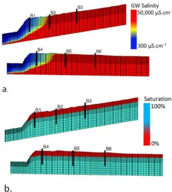
Fig. 4.3-D demonstration of simulated initial condition along tran-sects B1 and B2:(a)porous media saturation,(b)solute concentra-tion distribuconcentra-tion. Observaconcentra-tion wells are in black.
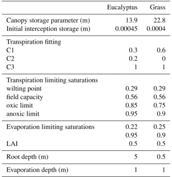
ET is one of the main drivers of the hydrological processes occurring in an arid/semi-arid region such as the lower River Murray (Doble et al., 2006; Holland et al., 2009a). The two main vegetation types occurring at the study site (Eucalyp-tus tree and grass) have significantly different characteris-tics in terms of root depth, water demand and leaf area in-dex. In order to obtain a better representation of the actual conditions, vegetation coverage of the floodplain was clas-sified into two different categories. Normalized evaporation and root depth functions were mapped onto porous media el-ements above the maximum depths. Currently, four evapora-tion and root depth funcevapora-tions are available in HGS; constant, linear, quadratic and cubic. In this study, quadratic evapora-tion and root depth funcevapora-tions were applied. Table 3 shows the values of the ET components for Eucalyptus and grass adopted from Hingston et al. (1997), Banks et al. (2011) and Verstrepen (2011).
Table 2.Surface properties values of the numerical model.
xfriction yfriction Rill storage Obstruction storage Coupling Longitudinal Transverse height (m) height (m) length (m) dispersivity (m) dispersivity (m)
River 0.005 0.005 0.0001 0 0.01 1 1
Floodplain 0.05 0.05 0.01 0.001 0.01 1 1
Fig. 5.Simulated and observed groundwater heads at observation wells.
Table 3.ET component parameters values for the study site.
Eucalyptus Grass
Canopy storage parameter (m) 13.9 22.8 Initial interception storage (m) 0.00045 0.0004
Transpiration fitting
C1 0.3 0.6
C2 0.2 0
C3 1 1
Transpiration limiting saturations
wilting point 0.29 0.29
field capacity 0.56 0.56
oxic limit 0.85 0.75
anoxic limit 0.95 0.9
Evaporation limiting saturations 0.22 0.25
0.95 0.9
LAI 0.5 0.5
Root depth (m) 5 0.5
Evaporation depth (m) 1 1
this regard, the observed water levels downstream of Lock 4 [ID: A42260515] (WaterConnect, 2013) were applied to the river nodes of the model. In addition, rainfall was simu-lated for the entire model surface domain beginning on day 1. ET was dynamically simulated as a combination of evap-oration and transpiration processes by removing water from all model cells of the surface and sub-surface flow domains
Table 4.Results of the calibrated model performance statistics.
Observation wells R2 Nr MSR (m) RMSE (m)
BO1 0.91 0.76 0.054 0.067
BO2 0.87 0.71 0.075 0.088
BO3 0.85 0.657 0.080 0.091
BO4 0.83 0.77 0.044 0.058
BO5 0.83 0.63 0.031 0.041
BO6 0.81 0.61 0.048 0.061
within the defined zone of the evaporation and root extinc-tion depths. The daily rainfall and potential evaporaextinc-tion val-ues used in the model were based on recorded daily rain-fall at the Loxton station [ID: 024024] (BOM, 2013). To represent the solute boundary conditions, first-type (Dirich-let) or constant concentration boundary conditions were as-signed. Observed groundwater TDS concentrations at the observation wells in the floodplain and river ranged from 30 000 mg L−1to 200 mg L−1. Hence, constant values were applied at the porous media boundary (representing the re-gional saline aquifer) and the river nodes accordingly. Fig-ure 3 illustrates the configuration of all boundary conditions in the model.
Fig. 6.Simulated solute concentration distribution(a)and EM31 survey (Berens et al., 2009)(b)in November 2007 at the study site.
Fig. 7. Groundwater heads at the boundary of the models (SIS wells) for the defined scenarios.
instance, if the field-observed data values are used as ini-tial conditions, the model response in the early time steps would reflect not only the model stress under study but also the adjustment of model head values to offset the lack of correspondence between model hydrologic inputs and pa-rameters and the initial head values (Franke et al., 1987). Therefore, in a transient state problem, the initial condi-tions should be determined through a steady/dynamic steady-state solution to generate dynamic cyclic initial conditions such as evaporation and rainfall seasonal cycles (Anderson and Woessner, 1992). Barnett et al. (2012) suggested carry-ing out a simulation which begins long enough before the calibration period allowing for an initial model equilibra-tion time. In this study, the stress period starts from 1 Jan-uary 2006 and ends on 1 September 2010. So, the initial model covers a 30 yr period to create the equilibrium ini-tial condition for the stress period. The iniini-tial model was intended to show equilibrium behaviour while its last time steps should be equal to the first time steps of the stress model which are observed (Fig. 4). Hence, simulated ground-water heads are compared with absolute observed values at observation wells (BO1: 10.4, BO2: 10.15, BO3: 10.01, BO4: 10.20, BO5: 10.14 and BO6: 10.07 mAHD; Holland et
Fig. 8.Changes in water storage in the porous media for the defined scenarios (light blue pattern refers to the period that the pumps were in operation).
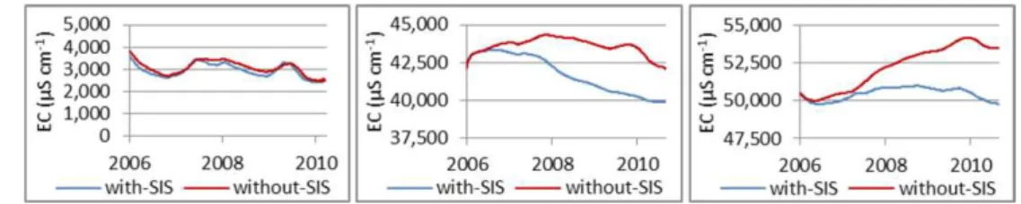
al., 2009b). Also, the status of the solute concentration dis-tribution at the beginning of the study (stress) period was checked with the general solute distribution pattern at the floodplain which was observed in the field and in related reports. This can be considered as two zones; a relatively fresh groundwater zone within 50 m distance of the river banks (BO1: 6500 µS cm−1 and BO4: 1200 µS cm−1) and a saline zone (BO2: 53 000 µS cm−1, BO3: 54 000 µS cm−1, BO5: 50 900 µS cm−1and BO6: 52 000 µS cm−1)for the rest of the floodplain (Holland et al., 2009b).
3.2 Coupled flow and transport calibration
Fig. 9.Water flux from the river to the floodplain aquifer for the defined scenarios (light blue pattern refers to the period that the pumps were in operation).
at the observation wells. But for the solute dynamic, given the difficulty associated with the quantification of the so-lute transport model parameters, the soso-lute was calibrated to the observed general salinity patterns of the floodplain aquifer. This was because concentration patterns are much more sensitive to local-scale geological heterogeneity than are hydraulic heads, and models may have difficulty repro-ducing the concentrations or their temporal variability at sin-gle observation wells. The general floodplain aquifer solute distribution was obtained from the EM31 surveys adopted from Berens et al. (2009). Hence, in this case, because of significant salinity differences between 50 m distance to the river bank (BO1 and BO4: EC<5000 µS cm−1)and the rest of the floodplain (BO2, BO3, BO5 and BO6: EC=30 000– 50 000 µS cm−1), an aggregate quantity like the plume mass is a more suitable calibration criterion, as recommended by Barnett et al. (2012).
Calibration of the model was conducted manually with more consideration to the sensitive parameters including soil hydraulic conductivity, porosity and dispersivity. The model performance for both flow and solute transport was tested by visual comparison between observed and simulated se-ries of hydraulic heads and solute concentrations at observa-tion wells BO1, BO2, BO3, BO4, BO5 and BO6. Moreover, quantitative evaluation was undertaken using goodness-of-fit measures. Figure 5 demonstrates the performance of the cal-ibrated model of Clark’s floodplain. Seeking to optimise the goodness-of-fit by minimizing errors between the observed and simulated values, or to achieve a specific predefined value of goodness-of-fit, may be the best way to increase con-fidence in predictions (Barnett et al., 2012). The goodness-of-fit measures, including root r-square (R2), Nash–Sutcliffe (Nr), mean sum of residuals (MSR) and root mean squared error (RMSE), are used to evaluate the simulated values against the observed data (Table 4). Moreover, the solute con-centration distribution results show that the calibrated model was able to reproduce the surface–groundwater interaction processes in an acceptable manner, as they present a good agreement. For instance, the EM31 survey in November 2007
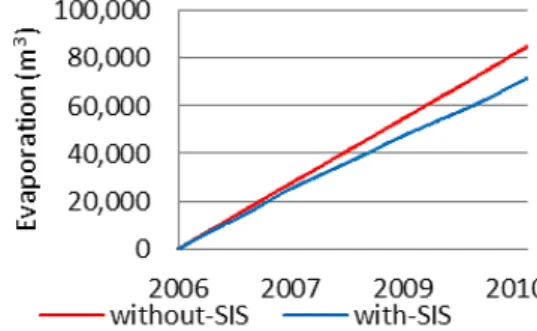
Fig. 10.Cumulative evaporation from the floodplain aquifer for the defined scenarios.
(Fig. 6a) showed a distinct zone of low conductivity along the eastern margin abutting the river channel. This shows the presence of freshwater within the floodplain aquifer (bank storage) and this was supported by groundwater salinity data collected at the riverbank piezometers at that time.
4 Results and discussion
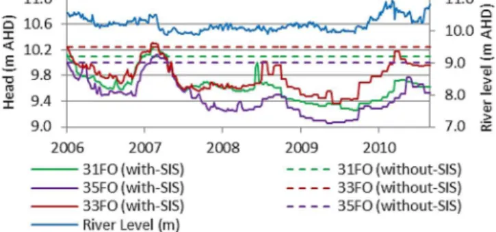
Fig. 11.Groundwater head dynamics at the observation wells on transect B1 for the with-SIS and the without-SIS scenarios.
Fig. 12.Groundwater head longitudinal profiles on 7 March 2007 (left), 16 November 2008 (middle) and 29 July 2009 (right) on transect B2 for the with-SIS and the without-SIS scenarios.
Fig. 13.Solute mass stored in the system in each time step for the defined scenarios. Cumulative pumped water is also shown in dark blue, and light blue pattern refers to the period that the pumps were in operation.
wells. In this paper, a losing floodplain regime corresponds to a movement of flow from the floodplain aquifer to the river and a gaining floodplain regime refers to flow movement from the river to the floodplain aquifer. Conversely, a losing river regime refers to movement of flow from the river to the floodplain aquifer and a gaining river shows flow movement from the floodplain aquifer to the river.
4.1 Water balance
One of the main starting points for analysis of the flow dy-namics in a surface–groundwater system is accurate mod-elling of the water balance. In this case, three forms of wa-ter balance outputs are considered as indicators to compare the scenarios. These indicators include changes in water stor-age in the porous and/or overland domain, the amount of water movement between the two domains (flow flux) and the groundwater head profile along the observation transects.
Hence, three outputs of the model are considered in the anal-ysis of the system water balance including the change in wa-ter storage (In-Out) in the porous medium (m3day−1), the water flux (m3)from the river to the floodplain aquifer and the groundwater head profile along transect B1.
Fig. 14.3-D visualization of solute mass changes in the unsaturated zone for the defined scenarios;(a)amount of solute mass removed from the unsaturated zone during the with-SIS scenario,(b)amount of solute mass that could be stored in the system if SIS was not installed on the floodplain.
production wells) to gaining (due to groundwater recharge). This shows that the river water level fluctuation is not the dominant driver in this situation; otherwise, an increase in accumulation rate would have occurred during the operation of the SIS production wells when the floodplain aquifer was in a losing regime.
Figure 9 shows the amount of water that moved from the river to the floodplain aquifer during the study period for the defined scenarios, and this is clearly related to the river water level. In other words, the amount of water that moves from the river to the floodplain aquifer increases with increasing river water levels and vice versa. This shows that for the study site there is a good connection between the river and the floodplain aquifer through bank recharge. On the other hand, the general trend in both scenarios is almost the same, although the amount of flux from the river to the floodplain aquifer is relatively higher for the with-SIS scenario. This is attributed to the operation of the SIS production wells that creates a groundwater gradient away from the river. In the with-SIS case, fresh river water is drawn towards the SIS production wells, which may result in a relatively fresher floodplain aquifer. It is worth noting that in a high river level
condition, which occurred at the end of the study period, a smaller difference in the flux is observed. This means that in high flow situations the amount of flux is too high for ground-water extraction (at least at this scale) to make a significant difference. Also, when the SIS was shut down from Novem-ber 2006 to May 2007, the flux from the river to the flood-plain was the same.
Fig. 15.Solute dynamics at the observation wells BO1 (left), BO2 (middle) and BO3 (right).
Fig. 16.Conceptual model of the impacts of groundwater extraction on salinization risk in a semi-arid floodplain.
4.2 Solute mass balance
Figure 13 shows the temporal trend of the total amount of solute mass stored in the system. The without-SIS scenario leads to a more saline floodplain aquifer, and also the amount of solute mass stored in the floodplain aquifer increases with time. In contrast, salinity levels were reduced for the with-SIS scenario with the exception of the period of time when the SIS was shut down. In fact, this was due to an increased flux of fresher river water induced by the SIS, in addition to the removal of saline groundwater and reduced saline groundwater flux to the floodplain from the highland. This is consistent with the field observations of Berens et al. (2009) and Holland et al. (2009b) at the same study site. Accord-ing to these results, the total solute mass stored in the system in the with-SIS scenario reduces by up to 4 % (1680 tonnes) while the without-SIS scenario shows a 2 % (846 tonnes) in-crease. Depending on the scale of the model, these values can be considerable. It is worth noting that in the without-SIS scenario, there is a relative decline in solute mass in the system at the end of the study period. This is due to the occur-rence of high river flows and overbank flows that took place just after the study period. Hence, in that short period, solute accumulation decreased and relatively less solute mass was stored in the system.
The unsaturated zone may act as an essential component of the solute mass stored in the floodplain aquifer, particu-larly in an area such as the study site where salinity is driven by increased discharge of saline groundwater and reduced leaching of salts from the soils. A high rate of ET can accel-erate this process. According to the results, at the last time step 7120 tonnes solute mass was stored in the unsaturated zone of the without-SIS model. The corresponding value for the with-SIS model for the same time step was 5562 tonnes. This proves that the groundwater extraction is able to remove a significant amount of solute stored in the unsaturated zone. It is worth noting that this model was up to 16 m in depth but shallower models might produce different proportions of un-saturated zone storage. Figure 14 illustrates the solute mass changes in the unsaturated zone for the defined scenarios. In Fig. 14a the distribution of solute mass removed from the unsaturated zone is shown. Groundwater extraction via the SIS operation removed solute mainly from the middle part of the floodplain. Figure 14b shows the amount of solute mass that could be stored in the system if the SIS was not installed on the floodplain. In fact, without groundwater ex-traction more solute could have been stored in the floodplain aquifer. This is consistent with the results in Fig. 13 which show that groundwater extraction may lead to a less saline floodplain as well as less solute mass storage in the unsatu-rated zone.
5 Conclusions
The relative impacts of saline groundwater extraction on the interactions between a river and its adjacent semi-arid flood-plain have been investigated. A 3-D fully integrated phys-ically based numerical model was used to simulate two de-fined scenarios, namely with and without SIS. The numerical model was first calibrated using observed data. The results showed a reasonable correlation between observed and simu-lated values. The model was able to effectively reproduce the surface–groundwater interactions. Then the calibrated model was used to simulate the defined without-SIS scenario. A conceptual model of the impact of groundwater extraction on floodplain salinization is shown in Fig. 16.
Water balance analysis showed that groundwater extrac-tion may change the floodplain aquifer regime from losing to gaining (or at least to reduce the losing rate). This happens by changing the head gradient towards the floodplain. This can lead to a higher amount of fresh river water flux to the saline floodplain aquifer and a wider freshwater lens along the riparian vegetation at the river bank. Also, a deeper wa-ter table is observed as a result of groundwawa-ter extraction. This is more significant in the area around the production wells in the floodplain rather than closer to the river banks. In the without-SIS scenario it is the river water fluctuations that dominate the surface–groundwater interactions while in the with-SIS scenario, the groundwater extraction is the main driver. Moreover, more groundwater has been removed from the floodplain aquifer via evaporation in the without-SIS sce-nario.
In terms of the solute balance, the SIS results in a less saline floodplain aquifer, as evidenced by the reduced amount of solute stored in the with-SIS scenario. Moreover, it was shown that groundwater extraction is able to remove significant proportions of the solute mass from the unsatu-rated zone. Overall, the saline groundwater extraction from the floodplain aquifer is shown to be an effective salt in-terception measure. This occurs through three mechanisms, namely extraction of the solute mass from the system, re-ducing the saline groundwater flux from the highland to the floodplain and changing the floodplain groundwater regime from a losing to a gaining one. The latter may result in more flux from the river to the floodplain aquifer. The current man-agement of the SIS operation seems to be effective in main-taining the floodplain salinity at a stable level.
Acknowledgements. This work was supported by the Goyder
In-stitute for Water Research. The authors would like to acknowledge the assistance and scientific support of Ian Jolly, Kate Holland and Rebecca Doble (CSIRO), Volmer Berens (DENWR), and Adrian Werner, Juliette Woods, James McCallum and Dylan Irvine (Flinders University).
Edited by: P. Tarolli
Reviewed by: A. Tolooiyan and one anonymous referee
References
Abbott, M. B., Bathurst, J. C., Cunge, J. A., O’Connell, P. E., and Rasmussen, J.: An introduction to the European Hydrological System—Syst‘eme Hydrologique Européen, SHE, 2: Structure of a physically-based distributed modeling system, J. Hydrol., 87, 61–77, 1986.
Allison, G. B., Cook, P. G., Barnett, S. R., Walker, G. R., Jolly, I. D., and Hughes, M. W.: Land clearance and river salinization in the western Murray Basin, Australia, J. Hydrol., 119, 1–20, 1990. Anderson, M. P. and Woessner, W. W.: Applied groundwater
mod-elling: simulation of flow and advective transport, Academic Press, San Diego, USA, 1992.
AquaVeo: GMS, Provo, UT, 2011.
Banks, E. W., Brunner, P., and Simmons, C. T.: Vegetation con-trols on variably saturated processes between surface water and groundwater and their impact on the state of connection, Water Resour. Res., 47, W11517, doi:10.1029/2011WR010544, 2011. Barnett, B., Townley, L. R., Post, V., Evans, R. E., Hunt, R. J.,
Peeters, L., Richardson, S., Werner, A. D., Knapton, A., and Boronkay, A.: Australian groundwater modelling guidelines, Na-tional Water Commission, Canberra, 2012.
Berens, V., White, M., and Souter, N.: Bookpurnong Living Mur-ray Pilot Project: A trial of three floodplain water management techniques to improve vegetation condition, Department of Wa-ter, Land and Biodiversity Conservation, Adelaide, 2009. Beven, K.: On explanatory depth and predictive power, Hydrol.
Pro-cess., 15, 3069–3072, 2001.
Beven, K.: Towards a coherent philosophy for modelling the envi-ronment, Proc. Roy. Soc. A, 458, 2465–2484, 2002.
Beven, K.: A manifesto for the equifinality thesis, J. Hydrol., 320, 18–36, 2006.
Beven, K. and Binley, A.: The future of distributed models: model calibration and uncertainty prediction, Hydrol. Process., 6, 279– 298, 1992.
BOM: Climate data online, available at: http://www.bom.gov.au, last access: 11 April 2013.
Brown, C. M. and Stephenson, A. E.: Geology of the Murray Basin, Southeastern, Bureau of Mineral Resources, Canberra, 1–22, 1991.
Brunner, P. and Simmons, C. T.: HydroGeoSphere: A Fully Inte-grated, Physically Based Hydrological Model, Ground Water, 50, 170–176, 2012.
Brutsaert, W. and Lopez, J. P.: Basin-scale geohydrologic drought flow features of riparian aquifers in the southern Great Plains, Water Resour. Res., 34, 233–240, 1998.
Camporese, M., Paniconi, C., Putti, M., and Orlandini, S.: Surface-subsurface flow modeling with path-based runoff routing, boundary condition-based coupling, and assimilation of mul-tisource observation data, Water Resour. Res., 46, W02512, doi:10.1029/2008WR007536, 2010.
Chen, X.: Stream water infiltration, bank storage, and storage zone changes due to stream-stage fluctuations, J. Hydrol., 280, 246– 264, 2003.
Chen, X. and Shu, L.: Groundwater evapotranspiration captured by seasonally pumped wells in river valleys, J. Hydrol., 318, 334– 347, 2006.
Physics and Earth Sciences, Flinders University of South Aus-tralia, Adelaide, 371 pp., 2004.
Doble, R., Simmons, C., Jolly, I., and Walker, G.: Spatial relation-ships between vegetation cover and irrigation-induced ground-water discharge on a semi-arid floodplain, Australia, J. Hydrol., 329, 75–97, doi:10.1016/j.jhydrol.2006.02.007, 2006.
DWR: South Australian River Murray Salinity Strategy 2001–2015, Department for Water Resources, Government of South Aus-tralia, Adelaide, 2001.
Ebel, B. A. and Loague, K.: Physics-based hydrologic-response simulation: Seeing through the fog of equifinality, Hydrol. Pro-cess., 20, 2887–2900, 2006.
Franke, O. L., Reily, T. E., and Bennett, G. D.: Definition of bound-ary and initial conditions in the anaysis of saturated ground-water flow systems; an introduction, USGS, Washington, 1–22, 1987. Freeze, R. A. and Harlan, R. L.: Blueprint for a physically-based,
digitally-simulated hydrologic response model, J. Hydrol., 9, 237–258, 1969.
Hart, B., Bailey, P., Edwards, R., Hortle, K., James, K., McMahon, A., Meredith, C., and Swadling, K.: A review of the salt sen-sitivity of the Australian freshwater biota, Hydrobiologia, 210, 105–144, 1991.
Herczeg, A. L., Simpson, H. J., and Mazor, E.: Transport of sol-uble salts in a large semiarid basin: River Murray, Australia, J. Hydrol., 144, 59–84, 1993.
Hingston, F. J., Galbraith, J. H., and Dimmock, G. M.: Applica-tion of the process-based model BIOMASS to Eucalyptus glob-ules subsp. Globglob-ules plantations on ex-farmland in south Western Australia: I. Water use by trees and assessing risk of losses due to drought., Forest Ecol. Manage., 106, 141–156, 1997. Hoehn, E. and Scholtis, A.: Exchange between a river and
ground-water, assessed with hydrochemical data, Hydrol. Earth Syst. Sci., 15, 983–988, doi:10.5194/hess-15-983-2011, 2011. Holland, K. L., Doody, T. M., McEwan, K. L., Jolly, I. D., White,
M., Berens, V., and Souter, N. J.: Response of the river murray floodplain to flooding and groundwater management: Field in-vestigations, CSIRO, Adelaide, 65, 2009a.
Holland, K. L., Jolly, I. D., Overton, I. C., and Walker, G. R.: An-alytical model of salinity risk from groundwater discharge in semi-arid, lowland floodplains, Hydrol. Process., 23, 3428–3439, 2009b.
HydroGeoLogic Inc: MODHMS: a comprehensive MODFLOW-based hydrologic modelling system, version 3.0, HydroGeo-Logic Incorporated, Herndon, USA, 2006.
Jarwal, S. D., Walker, G. R., and Jolly, I. D.: General site de-scription; Salt and Water Movement in the Chowilla Floodplain, CSIRO Division of Water Resources, 16-309, 1996.
Jolly, I. D., Walker, G. R., and Thorburn, P. J.: Salt accumulation in semi-arid floodplain soils with implications for forest health, J. Hydrol., 150, 589–614, doi:10.1016/0022-1694(93)90127-u, 1993.
Jolly, I. D., Walker, G. R., Hollingworth, I. D., Eldridge, S. R., Thor-burn, P. J., McEwan, K. L., and Hatton, T. J.: The causes of decline in eucalypt communities and possible ameliorative ap-proaches, in: Salt and Water Movement in the Chowilla Flood-plain, edited by: Walker, G. R., Jolly, I. D., and Jarwal, S. D., CSIRO Division of Water Resources, Canberra, Australia, 1996. Jolly, I. D., McEwan, K. L., and Holland, K. L.: A review of groundwater-surface water interactions in arid/semi-arid
wet-lands and the consequences of salinity for wetland ecology, Eco-hydrology, 1, 43–58, 2008.
Kollet, S. J. and Maxwell, R. M.: Integrated surface-groundwater flow modeling: A free-surface overland flow boundary condition in a parallel groundwater flow model, Adv. Water Resour., 29, 945–958, doi:10.1016/j.advwatres.2005.08.006, 2006.
Krause, S., Bronstert, A., and Zehe, E.: Groundwater-surface wa-ter inwa-teractions in a North German lowland floodplain – Implica-tions for the river discharge dynamics and riparian water balance, J. Hydrol., 347, 404–417, doi:10.1016/j.jhydrol.2007.09.028, 2007.
Kristensen, K. J. and Jensen, S. E.: A model for estimating ac-tual evapotranspiration from potential evapotranspiration, Nordic Hydrology, 6, 170–188, 1975.
Lamontagne, S., Leaney, F. W., and Herczeg, A. L.: Groundwater– surface water interactions in a large semi-arid floodplain: im-plications for salinity management, Hydrol. Process., 19, 3063– 3080, 2005.
Leavesley, G. H., Restrepo, P. J., Markstrom, S. L., Dixon, M., and Stannard, L. G.: The modular modeling system (MMS): User’s manual, USGS, Reston, Virginia, 1996.
Lenahan, M. J. and Bristow, K. L.: Understanding sub-surface solute distributions and salinization mechanisms in a tropical coastal floodplain groundwater system, J. Hydrol., 390, 131–142, doi:10.1016/j.jhydrol.2010.06.009, 2010.
Li, Q., Unger, A. J. A., Sudicky, E. A., Kassenaar, D., Wexler, E. J., and Shikaze, S.: Simulating the multi-seasonal response of a large-scale watershed with a 3D physically-based hydrologic model, J. Hydrol., 357, 317–336, 2008.
Liang, D., Falconer, R., and Lin, B.: Coupling surface and subsur-face flow in a depth averaged flood wave model, J. Hydrol., 337, 147–158, 2007.
Loague, K. and VanderKwaak, J. E.: Physics-based hydrologic re-sponse simulation: platinum bridge, 1958 Edsel, or useful tool?, Hydrol. Process., 16, 1015–1032, 2004.
McLaren, R. G.: Grid Builder: A pre-processor for 2-D, triangu-lar element, finite-element programs, Groundwater Simulations Group, University of Waterloo, Waterloo, Ontario, 2005. MDBA: Report of the Independent Audit Group for Salinity 2008–
2009, Murray-Darling Basin Authority (MDBA), Canberra, Aus-tralia, 2010.
Meire, D., De Doncker, L., Declercq, F., Buis, K., Troch, P., and Verhoeven, R.: Modelling river-floodplain interaction during flood propagation, Nat. Hazards, 55, 111–121, 2010.
Moench, A. F. and Barlow, P. M.: Aquifer response to stream-stage and recharge variations. I. Analytical step-response functions, J. Hydrol., 230, 192–210, 2000.
Nasonova, O. and Gusev, E.: Investigating the ability of a land surface model to reproduce river runoff with the accu-racy of hydrological models, Water Resources, 35, 493–501, doi:10.1134/s0097807808050011, 2008.
Overton, I. and Jolly, I.: Integrated studies of floodplain vegetation health, saline groundwater and flooding on the Chowilla flood-plain, South Australia, Integrated Studies of Floodplain Vegeta-tion Health, Saline Groundwater and Flooding on the Chowilla Floodplain South Australia, 2004.
Peck, A. J. and Hatton, T. : Salinity and the discharge of salts from catchments in Australia, J. Hydrol., 272, 191–202, 2003. Peck, A. J. and Hurle, D.H.: Chloride balance of some farmed and
forested catchments in Southwestern Australia, Water Resour. Res., 9, 648–657, 1973.
Petheram, C., Bristow, K. L., and Nelson, P. N.: Understanding and managing groundwater and salinity in a tropical conjunctive wa-ter use irrigation district, Agr. Wawa-ter Manage., 95, 1167–1179, 2008.
Pilgrim, D. H., Chapman, T. G., and Doran, D. G.: Problems of rainfall runoff modelling in arid and semi-arid regions, Hydrol. Sci. J., 33, 379–400, 1988.
Qu, Y. and Duffy, C. J.: A semidiscrete finite volume formulation for multiprocess watershed simulation, Water Resour. Res., 43, W08419, doi:10.1029/2006WR005752, 2007.
Rassam, D. W.: A conceptual framework for incorporating surface-groundwater interactions into a river operation-planning model, Environ. Model. Softw., 26, 1554–1567, 2011.
Ross, M. A., Tara, P. D., Geurink, J. S., and Stewart, M. T.: FIPR hydrologic model users’ manual and technical documentation, University of South Florida, Tampa, 1997.
Shlychkov, V.: Numerical modeling of river flows with account for vortex generation at the channel-floodplain boundary, Water Re-sources, 35, 522–529, doi:10.1134/s0097807808050035, 2008. Sophocleous, M.: Review: Groundwater management practices,
challenges, and innovations in the High Plains aquifer, USA-lessons and recommended actions, Revue critique: Pratiques, dé-fis et innovations dans le domaine des de la gestion des eaux souterraines de l’aquifère des Grandes Plaines (High Plains), aux Etats Unis d’Amérique - Leçons et recommandations, 18, 559– 575, 2010.
Sophocleous, M. S. and Perkins, P.: Methodology and application of combined watershed and ground-water models in Kansas, J. Hydrol., 236, 185–201, 2000.
Sophocleous, M., Koussis, A., Martin, J. L., and Perkins, S. P.: Eval-uation of simplified stream-aquifer depletion models for water rights administration, Ground Water, 33, 579–588, 1995. Squillace, P. J.: Observed and simulated movement of bank-storage
water, Ground Water, 34, 121–134, 1996.
Sun, D. and Zhan, H.: Pumping induced depletion from two streams, Adv. Water Reso., 30, 1016–1026, 2007.
Therrien, R.: Three-dimensional analysis of variablysaturated flow and solute transport in discretely-fractured porous media, Ph.D., University of Waterloo, Waterloo, 1992.
Therrien, R. and Sudicky, E. A.: Three-dimensional analysis of variably-saturated flow and solute transport in discretely-fractured porous media, J. Contaminant Hydrol., 23, 1–44, 1996. Therrien, R., McLaren, R. G., Sudicky, E. A., and Panday, S. M.: HydroGeoSphere: A Three-Dimensional Numerical Model De-scribing Fully-Integrated Subsurface and Surface Flow and So-lute Transport, Groundwater Simulations Group, University of Waterloo, Waterloo, Canada, 2005.
Therrien, R., McLaren, R. G., Sudicky, E. A., and Panday, S. M.: HydroGeoSphere; A Three-dimensional Numerical Model De-scribing Fully-integrated Subsurface and Surface Flow and So-lute Transport: User Manual, Groundwater Simulations Group, University of Waterloo, Waterloo, Ontario, Canada, 2010b. VanderKwaak, J. and Loague, K.: Hydrologic-response
simula-tions for the R-5 catchment with a comprehensive physics-based model, Water Resour. Res., 37, 999–1013, 2001.
VanderKwaak, J. E.: Numerical simulation of flow and chemical transport in integrated surface-subsurface hydrologic systems, PhD, University of Waterloo, Waterloo, Canada, 1999.
van Genuchten, M. T.: A closed-form equation for predicting the hydraulic conductivity of unsaturated soils, Sci. Soc. Am. J., 44, 892–898, 1980.
Verstrepen, L.: Evaluating rainwater harvesting on watershed level in the semi-arid zone of Chile, M.Sc., Bioscience Engineering, Universiteit Gent, Gent, 113 pp., 2011.
Viezzoli, A., Auken, E., and Munday, T.: Spatially constrained in-version for quasi 3D modelling of airborne electromagnetic data – an application for environmental assessment in the Lower Mur-ray Region of South Australia, Exploration Geophysics, 40, 173– 183, doi:10.1071/EG08027, 2009.
WaterConnect: River murray water data, available at: https://www. waterconnect.sa.gov.au, last access: 5 April 2013.
Wheater, H. S., Mathias, S. A., and Li, X.: Groundwater Modelling in Arid and Semi-Arid Areas, Cambridge University Press, 2010. White, M. G., Berens, V., and Souter, N. J.: Bookpurnong Living Murray Pilot Project: Artificial inundation of Eucalyptus camal-dulensis on a floodplain to improve vegetation condition, Sci-ence, Monitoring and Information Division, Department of Wa-ter, Land and Biodiversity Conservation, 2009.