Inference of Cross-Level Interaction between Genes and
Contextual Factors in a Matched Case-Control Metabolic
Syndrome Study: A Bayesian Approach
Shi-Heng Wang1, Wei J. Chen1,2,3, Lee-Ming Chuang4,5, Po-Chang Hsiao1,2, Pi-Hua Liu6, Chuhsing K. Hsiao1,3,7*
1Institute of Epidemiology and Preventive Medicine, College of Public Health, National Taiwan University, Taipei, Taiwan,2Genetic Epidemiology Core Laboratory, Center of Genomic Medicine, National Taiwan University, Taipei, Taiwan,3Department of Public Health, College of Public Health, National Taiwan University, Taipei, Taiwan, 4Department of Internal Medicine, National Taiwan University Hospital, Taipei, Taiwan,5Institute of Clinical Medicine, College of Medicine, National Taiwan University, Taipei, Taiwan,6Clinical Informatics and Medical Statistics Research Center, Chang Gung University, Guishan, Taiwan,7Bioinformatics and Biostatistics Core, Center of Genomic Medicine, National Taiwan University, Taipei, Taiwan
Abstract
Genes, environment, and the interaction between them are each known to play an important role in the risk for developing complex diseases such as metabolic syndrome. For environmental factors, most studies focused on the measurements observed at the individual level, and therefore can only consider the gene-environment interaction at the same individual scale. Indeed the group-level (called contextual) environmental variables, such as community factors and the degree of local area development, may modify the genetic effect as well. To examine such cross-level interaction between genes and contextual factors, a flexible statistical model quantifying the variability of the genetic effects across different categories of the contextual variable is in need. With a Bayesian generalized linear mixed-effects model with an unconditional likelihood, we investigate whether the individual genetic effect is modified by the group-level residential environment factor in a matched case-control metabolic syndrome study. Such cross-level interaction is evaluated by examining the heterogeneity in allelic effects under various contextual categories, based on posterior samples from Markov chain Monte Carlo methods. The Bayesian analysis indicates that the effect of rs1801282 on metabolic syndrome development is modified by the contextual environmental factor. That is, even among individuals with the same genetic component ofPPARG_Pro12Ala, living in a residential area with low availability of exercise facilities may result in higher risk. The modification of the group-level environment factors on the individual genetic attributes can be essential, and this Bayesian model is able to provide a quantitative assessment for such cross-level interaction. The Bayesian inference based on the full likelihood is flexible with any phenotype, and easy to implement computationally. This model has a wide applicability and may help unravel the complexity in development of complex diseases.
Citation:Wang S-H, Chen WJ, Chuang L-M, Hsiao P-C, Liu P-H, et al. (2013) Inference of Cross-Level Interaction between Genes and Contextual Factors in a Matched Case-Control Metabolic Syndrome Study: A Bayesian Approach. PLoS ONE 8(2): e56693. doi:10.1371/journal.pone.0056693
Editor:Giuseppe Novelli, Tor Vergata University of Rome, Italy
ReceivedAugust 20, 2012;AcceptedJanuary 14, 2013;PublishedFebruary 20, 2013
Copyright:ß2013 Wang et al. This is an open-access article distributed under the terms of the Creative Commons Attribution License, which permits unrestricted use, distribution, and reproduction in any medium, provided the original author and source are credited.
Funding:This research was supported in part by NSC 100-2314-B-002-107-MY3, NSC 97-2314-B-002-040-MY3, DOH 94-TD-G-111-036, 94HDI002, and National Taiwan University Center of Genomic Medicine. The funders had no role in study design, data collection and analysis, decision to publish, or preparation of the manuscript. WJC and CKH thank the support of Research Center for Genes, Environment and Human Health in College of Public Health, National Taiwan University.
Competing Interests:The authors have declared that no competing interests exist.
* E-mail: [email protected]
Introduction
Both genetic and environmental factors play an important role in the development of many diseases, often interacting in ways that elevate disease risk, especially in complex diseases such as obesity, cardiovascular disease, and psychopathology [1–3]. To investigate genetic and environmental (GE) interactions [4–6], many studies have focused on environmental factors measured at the individual level, such as individual demographic information or lifestyle. It is possible, however, that group-level environmental factors, usually called contextual variables, also contribute to such risk. For instance, community disparity in medical resources may affect the availability and quality of treatment, and therefore living in a deprived area may result in a somewhat modified effect on the health risk incurred by individuals who engage in unhealthy
behaviors such as smoking [7]. This contextual exposure affects the individual health status of each member of the group, and is therefore called thecontextual effect[8,9].
interaction. These issues differ from what has been considered in most current research where GE interaction is evaluated at the individual level based on a case-control study design. For cross-level GE interaction in clustered data, one immediate computa-tional complexity involves the existence of multiple sources of variation. For example, homogeneity among individuals in the same group may produce dependence [8], whereas the corre-sponding matched controls for any case may induce further correlation. In addition, the genetic effects may be modified by group-level exposures and may, therefore, correlate with each other. These nested sources of variability hamper the model construction and parameter inference. Several research groups adopted Bayesian or non-Bayesian hierarchical models to alleviate the problem of nested variability [10,11], but these models are not for matched case-control studies and not for group-level GE interaction [12–15].
To accommodate the nested structure of variation in both the individual- and group-level variables, and to model directly the interaction between individual genetic factors and group-specific variables, Bayesian hierarchical models with random effects can be formulated for inference. By employing hierarchical models with mixed effects, inference of these multiple variance components becomes feasible and may help elucidate whether cross-level interaction does exist, and/or quantify the strength of this interaction from a probabilistic perspective based on posterior distributions.
This research was motivated by a matched case-control study of metabolic syndrome [16], a condition which is characterized by a group of metabolic conditions and risk factors. In that metabolic disorder study, the effects of community exercise facility as well as five candidate SNPs (rs1801282, rs7799039, rs12535708, rs822390, and rs182052) were investigated. These factors were selected based on previous publications of association studies linking them to obesity and body mass index (BMI). Many studies have recognized the association between metabolic disorder and both diabetes and coronary heart disease [17,18], while a few studies have shown that both genes and contextual variables, such as community disadvantage, income inequality, and factors affecting community development [19–22], associate strongly with the risk of metabolic syndrome. In a densely populated country such as Taiwan where the boundary between residential areas and commercial districts is blurred, an individual household may not have enough space for exercise. Even at the community level, there may not be sufficient exercise facilities such as gymnasiums, track fields, parks, or playgrounds for residents to use. This may restrict an individual’s accessibility to an exercise facility and influence one’s degree of physical inactivity. Although such group-level environmental variables can exert an effect on the risk of metabolic syndrome in addition to the effect exerted by individual environmental factors [19–23], it is not certain whether the contextual variable will interact with the genetic effect in the same manner as the individual environmental variable does [24–29]. In the rest of this article, we reserve the abbreviation GE for the cross-level interaction at the contextual-level, and Ge for the gene-environment interaction at the individual-level.
The purpose of this paper is to explore the cross-level GE interaction in this matched case-control study via a Bayesian hierarchical model with an unconditional likelihood approach. We illustrate our approach with the aforementioned study concerning five candidate SNPs and GE which involves a contextual variable measuring the availability of exercise facilities. The posterior samples of the parameters of interest, the group-specific random effects and the variance among them, will be used to examine the existence of cross-level GE interaction.
Methods
Motivating Example: The Metabolic Syndrome Study This study was conducted by Wang and colleagues in Tao-Yuan County in Taiwan in 2004 [16]. Here we briefly summarize the collection procedures of samples, while other details are referred to their original paper. This study recruited 6463 community residents aged greater than 40 years old in an adult health check-up program, and collected a questionnaire and blood sample from each participant. Among the recruited subjects, 1263 were classified with metabolic syndrome based on US National Cholesterol Education Program Adult Treatment Panel III (NCEP ATP III) criteria, with BMI replacing waist measurements. That is, an individual was considered to have metabolic disorder if three or more of the following criteria were met: BMI $ 27 kg/m2; triglycerides $ 150 mg/dl; HDL ,40 mg/dL in men and
,50 mg/dL in women; blood pressure $ 130/85 mmHg or medication for hypertension currently taken; and fasting glucose$
110 mg/dL or medication for diabetes currently taken. Next, two hundred- and sixty-eight cases were randomly selected and matched with one or two controls by sex, age, educational level, ethnicity, and a contextual variable measuring the availability of exercise facilities. Exercise facilities included swimming pools, parks, bowling alleys, golf courses, fitness centers, and activity centers for the elderly. For each residential area, the exercise facility density was defined as the number of facilities divided by the number of residents, and this density was categorized into four different levels of availability in exercise facility: level I for very low availability, II for low, III for medium, and IV for high. The final data set for analysis contained 268 metabolic syndrome cases and 322 individually matched controls. The terms ‘‘cases’’ and ‘‘controls’’ here do not intend to indicate that metabolic syndrome is a disease. It is indeed a group of metabolic conditions that associate strongly with increased risk of cardiovascular disease and diabetes. In other words,metabolic syndrome is a clustering of risk factors. Discussions and debates about its definition, inclusion criteria, and usefulness in clinical practice have drawn much attention [30,31]. Here we call these identified individuals ‘‘cases’’ simply for ease of presentation.
Candidate Genes and Odds Ratios
cross-level interaction between rs1801282 and exercise facility availability in the residential environment.
Bayesian Hierarchical Model with Unconditional Likelihood
To examine if the effect of the SNP rs1801282 varies among different categories of the contextual covariate, along with the SNP-SNP interaction between rs12535708 and rs7799039 in the same geneLEPon 7q31, we adopt a Bayesian generalized linear mixed-effects model (GLMM). This Bayesian GLMM assumes that each response variable Yijk, the binary disease status (1 for
case and 0 for control) of thek-th individual in thej-th pair of the i-th category, follows a Bernoulli distribution with the parameter pijkindicating the probability of having metabolic syndrome,
YijkDpijk*Bernoulli pijk
,
where the probability of being diseasedpijkis associated in the logit
scale with the 5 (SNP) genetic componentsS(1),:::,S(5) (following the same order and coding as in Table 1) and a SNP–SNP interactionS(2,3), in addition to other covariatesX,
logit pijk
~X
5
g~1
b(ig)|S(ijkg)zc|Sijk(2,3)zh|Xijkzbizbij:
The implication of each parameter is explained in the following paragraphs, and outlined in the supporting information Table S1. All considered explanatory variables are summarized as well.
Cross-level GE Interaction
The covariateSijk(g)indicates the coding of the SNPgfor thek-th individual in the j-th pair of the i-th category. Its associating parameterb(ig) represents the SNP effect under thei-th category for the SNPg. For instance, the evaluation and comparison of the 4 (i~1,:::,4) posterior distributions ofb(1)1 ,b(1)2 ,b(1)3 , andb(1)4 can reveal if the effect of the first SNP (g= 1) rs1801282 varies among the 4 different categories of the contextual covariate. Therefore, the variance var(b(ig)) =s2
(g)can model directly the heterogeneity in SNP effects among 4 categories for each SNPg. This variance measures the degree to which the genetic effect differs across different categories of the contextual variable. This is thus the parameter of interest when the cross-level GE interaction is to be evaluated.
SNP-SNP Interaction and Other Effects
The SNP-SNP interaction between the second SNP rs7799039 and the third SNP rs12535708 in the same gene is measured byc. The parameter h represents the effect of other explanatory variable X. The random intercept bi stands for the category-specific effect accounting for the sampling variability among residential areas. The second random interceptbij is for the pair-or cluster-specific random effect. Thisbij represents the matching relation within each pair. In other words, subjects in the same pair share the same baseline characteristics and pairs are taken to be independent. The random coefficients are all assumed to follow normal distributions with a large variance representing vague information. A complete model specification including all prior distributions is detailed in the supporting information (Text S1).
Computation
The analysis was conducted based on posterior samples obtained from Markov chain Monte Carlo (MCMC) methods with WinBUGS 1.4.3. The chain contained 50,000 iterations following a burn-in of 5,000 samples to reduce the impact from initial values and the final posterior sample was derived at the thinning rate of 10 to reduce dependence among posterior points. The code in WinBUGS is detailed in the supporting information (Text S2).
Results
Cross-level Gene-Environment Interaction
To investigate the existence of the cross-level GE interaction, we list in Table 2 the posterior means and standard deviations of thei -th category-specific genetic effectsb(ig) and variances2
(g)for each SNPg, and display the posterior distributions of theb(ig)for SNPs
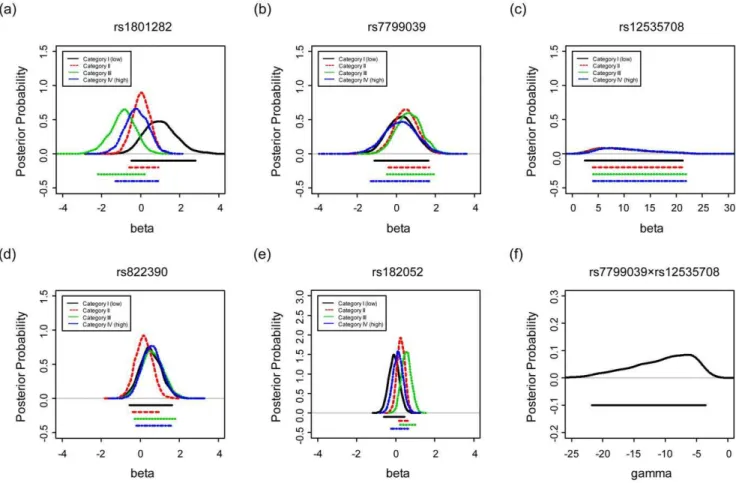
g= 1, …, 5 in Figure 1(a)–(e). From Table 2, it is apparent that for rs1801282 (g= 1) the four category-specific meansb(ig),i~1,:::,4, differ the most. This implies a relatively large variation of genetic effect across the 4 areas. The same pattern can be observed in the
Table 1.The observed genotype counts of metabolic cases
(cs) and controls (cn) under each category of exercise facility availability.
Category Total
SNP I II III IV
genotypes
(coding) cs/cn cs/cn cs/cn cs/cnl cs/cn
S(1), rs1801282,PPARG_Pro12Ala
C/C (0) 46/52 84/109 63/68 51/64 244/293
C/G (1) 5/1 10/13 4/8 5/7 24/29
Conditional OR 5.7 0.9 0.7 0.9
S(2), rs7799039,LEP_G2548A
A/A, A/G (0) 40/45 77/108 54/69 42/62 213/281
G/G (1) 11/8 17/17 13/7 14/9 55/41
Conditional OR 1.4 1.4 2.7 3.3
S(3), rs12535708,LEP_H1328082
C/C, C/A (0) 50/50 83/114 60/73 52/68 245/305
A/A (1) 1/3 11/8 7/3 3/4 23/17
Conditional OR 0.4 2.3 2.9 1.8
S(4), rs822390,APM1_G_7950T
T/T (0) 41/47 83/114 58/72 45/65 227/298
T/G (1) 6/5 6/4 6/4 2/3 20/16
G/G (2) 4/1 5/4 3/0 9/3 21/8
Conditional OR 1.7 1.6 3.2 2.0
S(5), rs182052,APM1_A_10066G
A/A (0) 6/8 13/26 7/18 11/15 37/67
A/G (1) 28/23 46/62 30/38 25/38 129/161
G/G (2) 17/22 35/34 30/20 20/18 102/94
Conditional OR 0.9 1.5 1.8 1.3
Total 51/53 94/122 67/76 56/71 268/322
corresponding four posterior distributions ofb(ig)in Figure 1. The curves in Figure 1(a) are more scattered, as compared with the other four plots (Figure 1(b), (c), (d) and (e)), indicating substantially larger heterogeneity in the genetic effect of rs1801282 across the four categories. Another supporting evidence lies in the inference ofs2
(g)forg= 1, …, 5. The last column in Table 2 lists the posterior means ofs2
(g)where the first SNP rs1801282 has the largest mean (1.31), implying again a larger heterogeneity. Figure 2 displays their corresponding distributions. Indeed,s2
(g)for rs1801282 is the most right skewed, representing an observable difference among areas. Further evidence manifests through the evaluation of the difference in risk across the four categories. For instance, for SNP
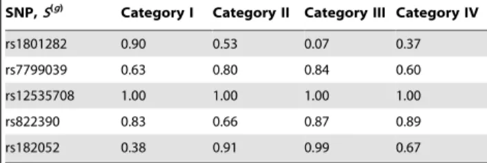
g= 1, if the posterior probabilities of the risk, P(b(1)1 .0|y), P(b(1)2 .0| y), P(b(1)3 .0| y), and P(b(1)4 .0| y), deviate from each other, then this SNP has divergent effects among areas. Again, for rs1801282, the corresponding four posterior probabilities contain the largest degree of variation (Table 3).
These findings consistently imply the existence of the cross-level interaction between this SNP and the contextual variable. To be specific, the analyses suggest that, even among those residents with the same genotype C/G for rs1801282, living in an area with low availability of exercise facilities (category I) leads to a higher risk of being metabolically diseased. In other words, the G allele (also called the Ala allele inPPARG_Pro12Ala) is considered protective under categories II-IV, but not under category I. In fact, we have conducted Bayesian model selection using the deviance informa-tion criterion (DIC) to compare the model with GE interacinforma-tion
and without (assumingb(1)1 ~b(1)2 ~b(1)3 ~b(1)4 ). The former model containing the cross-level GE interaction term was selected.
This pattern of interaction, however, is not shown for other SNPs. For example, the second SNP (rs7799039) in Figure 1(b) and the fourth SNP (rs822390) in Figure 1(d) reveal only mild variation; while the third SNP (rs12535708) in Figure 1(c) and the
Figure 1. The posterior distributions ofb(ig) (i= 1,…,4) for four categories are displayed in (a)–(e) for SNPg= 1, g= 2,…,g= 5, respectively, under the Bayesian unconditional likelihood model.
doi:10.1371/journal.pone.0056693.g001
Figure 2. The posterior distributions ofs2
(g)forg= 1, …, 5 SNP, respectively, under the Bayesian unconditional likelihood model.
fifth SNP (rs182052) in Figure 1(e) show almost no difference in the 95% credible intervals across the four categories. In addition, the density functions of s2
(1), s2(2), …, and s2(5) differ from each other, which implies different patterns in heterogeneity among the 5 SNPs.
SNP-SNP Interaction
To evaluate the existence of interaction between SNPs, we examine the posterior distribution of c for the SNP-SNP interaction between rs7799039 and rs12535708. Notice that the posterior distribution of cis left-skewed with a mean of210.70 and a 95% credible interval (221.8,23.5), indicating a protective effect when these two SNPs simultaneously carry the G/G and A/ A genotypes, respectively (Table 2 and Figure 1(f)). The overall aggregation of effects, however, shrinks toward zero when accounting for both single-SNP effects. For instance, in category I, the sum of the average odds ratios for genotype G/G for rs7799039, A/A for rs12535708, and their interaction is about exp(0.25+9.90–10.70) = exp(20.55), resulting in an odds ratio of approximately 0.58( = exp(20.55)). In other words, the interaction diminishes the two strong first-order genetic effects.
Discussion
The research reported here was motivated by a matched case-control metabolic syndrome study where interest lay in the interaction between genes and contextual variables, as well as SNP-SNP interaction. Such cross-level GE interaction can be as important as the individual level Ge interaction, and thus its influence should not be overlooked. The statistical inference of GE, however, is not straightforward. We adopted here a Bayesian
model with random effects to investigate the genetic and environmental interactions by examining the extent to which the allelic effects differ across various categories of the contextual variable. Though many studies have been proposed to test the interaction between genes and environment at the individual level, this Bayesian approach, to the best of our knowledge, is the first Bayesian analysis to infer the cross-level interaction between individual genetic and contextual residential area effects. The advantages of employing a Bayesian unconditional likelihood model are its flexibility in model construction for complex models; the straightforwardness in deriving the posterior distribution of the variance s2
g to assess cross-level interaction; and the ability to
estimate multidimensional parameters simultaneously.
Biological Implications
The results indicated that the effect of rs1801282 is likely to be modified by the contextual factor in the sense that individuals with the mutant genotype have higher risk, particularly when living in an area with low availability of exercise facilities. On the basis of the large posterior variability in genetic effects across areas, we conclude that this effect is modulated by the residential environmental factor. Similar observations have been previously reported in other studies where the rs1801282 SNP was shown to exacerbate the negative effect of poor individual exercise habits [24–27]. Others have observed that physical inactivity and sedentary lifestyle may interfere with optimized expression of the ‘‘thrifty’’ genes [28] and that the availability of recreational resources can relate directly to an individual’s physical activity level [39]. These findings are in agreement with our finding that the availability of recreational resources will interact with the effect of rs1801282 on metabolic syndrome in such a way that living in areas with lower exercise facility availability will increase the risk of disease, particularly for individuals carrying the mutant type of rs1801282.
The model we have introduced here for the matched design can accommodate SNP-SNP interaction as well. For instance, SNPs rs12535708 and rs7799039 locate closely in the gene LEP on chromosome 7q31, where rs7799039 is in the 59 regulatory promoter region and rs12535708 is at the transcription-factor binding site. The strong LD between these two SNPs has been documented earlier [40], and the existence of their statistical interaction indicates that these two SNPs may be involved in similar functional pathways. An existing study reported that rs7799039 cannot add further information when other multi-marker haplotypes containing rs12535708 have been included for analysis [40]. Our results replicate the finding that, when both SNPs are present in the model, rs12535708 exhibits strong association (the posterior modes ofb(3)1 *b(3)4 are all around 10), while the influence of rs7799039 is mild (posterior modes of Table 2.In the upper half of the table, numbers in each row
are the posterior means and standard deviations of the area-specific genetic effects (b(ig)) and variance (Var(b(ig)) =s2
(g)) for each candidate SNPg.
Posterior mean (se)
SNP Covariatesb(1g), I b (g) 2, II b
(g) 3, III b
(g)
4 , IV s2(g)
S(1), rs1801282 (PPARG_Pro12Ala)
1.01 (0.83) 0.03 (0.45) 20.91 (0.66) 20.20 (0.60) 1.31 (0.94)
S(2), rs7799039 (LEP_G2548A)
0.25 (0.71) 0.49 (0.60) 0.65 (0.65) 0.21 (0.84) 1.03 (0.68)
S(3), rs12535708 (LEP_H1328082)
9.90 (5.11) 10.02 (5.06) 10.71 (5.09) 10.92 (5.11) 1.22 (0.84)
S(4), rs822390 (APM1_G-7950T)
0.52 (0.55) 0.18 (0.44) 0.64 (0.57) 0.61 (0.52) 0.97 (0.64)
S(5), rs182052 (APM1_A-10066G)
20.08 (0.27) 0.27 (0.20) 0.54 (0.25) 0.12 (0.26) 0.91 (0.56) SNP-SNP interaction
S(2,3), rs77990396rs12535708 c 210.70 (5.06)
Other variance components
Among areas, Var(bi) s2area 0.62
(0.40)
Among pairs, Var(bij) s2pair 0.22
(0.05)
The bottom half of the table contains posterior means and standard deviations for parameters of the SNP-SNP interaction, and for variance component parameters.
doi:10.1371/journal.pone.0056693.t002
Table 3.Numbers areP(b(ig)w0Dy), the posterior probability
of(b(ig)w0), for theg-th SNP in thei-th category (area) under
the unconditional model.
SNP,S(g)
Category I Category II Category III Category IV
rs1801282 0.90 0.53 0.07 0.37
rs7799039 0.63 0.80 0.84 0.60
rs12535708 1.00 1.00 1.00 1.00
rs822390 0.83 0.66 0.87 0.89
rs182052 0.38 0.91 0.99 0.67
b(2)1 *b(2)4 are between 0 and 1). When accounting for both markers along with their interaction, the estimated odds ratios of being metabolic, for persons carrying genotype G/G for rs7799039 and A/A for rs12535708, are 0.57, 0.83, 1.02, and 1.54 for the four categories, respectively. Each of the resulting values implies the existence of SNP-SNP interaction, and the heterogeneity among the four odds ratios provides evidence for GE interaction. Further research about the functional polymor-phism of these two SNPs, or haplotype analysis, would be worth pursuing to unravel their biological interplay.
Other Statistical Models for GE interaction
1. Bayesian conditional logistic regression model. If only some of the previously mentioned parameters are of interest, then their inference can be made under the Bayesian conditional logistic regression (BCLR) model assumingpijk=eijk=Pkeijk, and
a log link formulation oneijk
logeijk~
X5
g~1
b(ig)|S(ijkg)zc|S(2,3)ijk zh|Xijk,
where for each SNPg,b(ig)NormalN~ m(g),s2 (g)
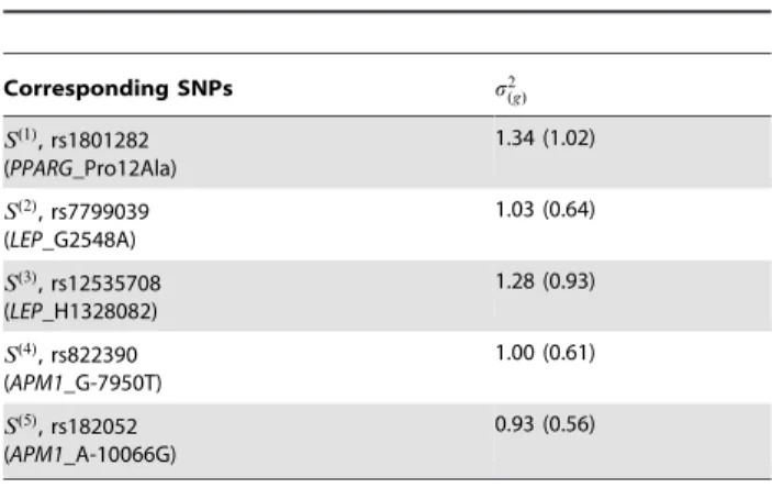
,i~1,:::,4. Table S2 displays the model and parameters for comparison. Table 4 lists the posterior means and standard errors ofs2
(g)forg~1,:::,5. The posterior distributions of s2
(g) under the Bayesian conditional logistic regression do not vary much from that under the Bayesian unconditional likelihood model. In addition, we have investigated the pattern based on a limited simulation study with only 10 replications, each containing five SNPs for 100 cases and 100 matched controls in every one of the 4 areas. The consistency in the inference of variance between the Bayesian unconditional and conditional models stays clearly. However, as compared with the previous unconditional model, the disadvantages are that one is unable to infer the sampling variability among areas or within each pair under this BCLR, and the computational difficulty is greatly elevated under this setting if the number of genetic markers is large. Our experience shows that even when the computation under BCLR reaches convergence, the computation time for BCLR is about 4.5 times that of the Bayesian full likelihood model, when computed with an Intel core i7-2620M (2.7/3.4GHz) dual-core processor.
Although the BCLR model could be viewed as a workable alternative model in this case, its computational burden and lack of information on sampling variability within clusters hinder its use in such a cross-level GE study. The unconditional likelihood approach uses matched-pair specific random effects to account for the selection bias, while the conditional approach adopts matched-pair specific intercepts [41]. Another reason for favoring the Bayesian unconditional likelihood approach is that the full likelihood model can accommodate complex nested structures easily and intuitively, such as those involving matched cases and controls in the same category. These various sources of dependence can be modeled straightforwardly.
2. Models with cross-product terms. Other alternative for handling the cross-level GE interaction in a matched design is through the use of cross-product terms of dummy variables for areas and SNP covariates. Some possibilities are outlined in the supporting information (Text S3).
We do not recommend however the use of these other models with cross-product terms, because the large number of coefficients of GE interaction often leads to failure in the MCMC computations. Other non-Bayesian multi-level models with the
MQL option in MLwiN and glmmPQL in R are theoretically possible, but the computation for this matched case-control metabolic syndrome study collapses when it runs into a non-positive definite matrix during the iteration procedure.
Further Notes
Some further notes are worth mentioning. First, for the sensitivity analysis of the posterior inference, we have tried other prior distributions. For example, we have used different gamma distributions for the precision parameters (the inverse of the variance components), and obtained similar conclusions. Sec-ond, we have adopted a Bayesian hierarchical model with no GE interaction for rs1801282, and performed model selection with DIC. The model with the cross-level GE was selected, and therefore the posterior probability under the GE model was evaluated for inference. Last but not least, although Bayesian models may at first seem complicated with respect to their formulation and computation, the advancement of MCMC methods has greatly enhanced the feasibility of using Bayesian inference in daily practice. Several software applications, such as WinBUGS, R, and MLWin, are handy for carrying out Bayesian analysis. The model presented here for analyzing interaction between genes and contextual variables could achieve broad applicability with the aid of these statistical analysis tools.
Supporting Information
Table S1 The formulation and parameter
interpreta-tion of the uncondiinterpreta-tional likelihood Bayesian model. (DOCX)
Table S2 The formulation and parameter
interpreta-tion of the Bayesian condiinterpreta-tional logistic regression model.
(DOCX)
Text S1 Complete specification of the Bayesian model.
(DOC)
Text S2 WinBUGS code of the Bayesian model.
(DOCX)
Table 4.The variance parameters represent the variability among areas for each SNP.
Corresponding SNPs s2
(g)
S(1), rs1801282 (PPARG_Pro12Ala)
1.34 (1.02)
S(2), rs7799039 (LEP_G2548A)
1.03 (0.64)
S(3), rs12535708 (LEP_H1328082)
1.28 (0.93)
S(4), rs822390 (APM1_G-7950T)
1.00 (0.61)
S(5), rs182052 (APM1_A-10066G)
0.93 (0.56)
Numbers are posterior means and standard deviations of variance components under the Bayesian conditional logistic regression model.
Text S3 Model formulation and parameter interpreta-tions with cross-product terms for cross-level interac-tion.
(DOCX)
Author Contributions
Conceived and designed the experiments: CKH WJC LMC. Performed the experiments: PHL. Analyzed the data: SHW PCH. Contributed reagents/materials/analysis tools: CKH WJC LMC. Wrote the paper: SHW LMC CKH.
References
1. Qi L, Cho YA (2008) Gene-environment interaction and obesity. Nutr Rev 66: 684–694.
2. Stephens JW, Bain SC, Humphries SE (2008) Gene-environment interaction and oxidative stress in cardiovascular disease. Atherosclerosis 200: 229–238. 3. Thapar A, Harold G, Rice F, Langley K, O’Donovan M (2007) The
contribution of gene-environment interaction to psychopathology. Dev Psycho-pathol 19: 989–1004.
4. Dempfle A, Scherag A, Hein R, Beckmann L, Chang-Claude J, et al. (2008) Gene-environment interactions for complex traits: definitions, methodological requirements and challenges. Eur J Hum Genet 16: 1164–1172.
5. Greenland S (2009) Interactions in epidemiology: relevance, identification, and estimation. Epidemiology 20: 14–17.
6. Rutter M (2008) Biological implications of gene-environment interaction. J Abnorm Child Psychol 36: 969–975.
7. Blakely TA, Woodward AJ (2000) Ecological effects in multi-level studies. J Epidemiol Community Health 54: 367–374.
8. Diez Roux AV (2002) A glossary for multilevel analysis. J Epidemiol Community Health 56: 588–594.
9. Greenland S (2001) Ecologic versus individual-level sources of bias in ecologic estimates of contextual health effects. Int J Epidemiol 30: 1343–1350. 10. Parnell AC, Inger R, Bearhop S, Jackson AL (2010) Source partitioning using
stable isotopes: coping with too much variation. PLoS ONE 5: e9672. doi:9610.1371/journal.pone.0009672.
11. Semmens BX, Ward EJ, Moore JW, Darimont CT (2009) Quantifying inter-and intra-population niche variability using hierarchical bayesian stable isotope mixing models. PLoS ONE 4: e6187. doi:6110.1371/journal.pone.0006187. 12. Aragaki CC, Greenland S, Probst-Hensch N, Haile RW (1997) Hierarchical
modeling of gene-environment interactions: estimating NAT2 genotype-specific dietary effects on adenomatous polyps. Cancer Epidemiology, Biomarkers & Prevention 6: 307–314.
13. Hung RJ, Brennan P, Malaveille C, Porru S, Donato F, et al. (2004) Using hierarchical modeling in genetic association studies with multiple markers: application to a case-control study of bladder cancer. Cancer Epidemiology, Biomarkers & Prevention 13: 1013–1021.
14. Wakefield J, De Vocht F, Hung RJ (2010) Bayesian mixture modeling of gene-environment and gene-gene interactions. Genetic Epidemiology 34: 16–25. 15. Yu K, Wacholder S, Wheeler W, Wang Z, Caporaso N, et al. (2012) A flexible
Bayesian model for studying gene-environment interaction. PLoS Genetics 8: e1002482.
16. Wang SH, Hsiao PC, Hsiao CK, Liu PH, Chien KL, et al. (2011) Multilevel analysis of habitual physical activity and metabolic syndrome in Northern Taiwan. Prev Med: doi:10.1016/j.ypmed.2011.1004.1017.
17. Eckel RH, Grundy SM, Zimmet PZ (2005) The metabolic syndrome. Lancet 365: 1415–1428.
18. Zimmet P, Alberti KGMM, Shaw J (2001) Global and societal implications of the diabetes epidemic. Nature 414: 782–787.
19. Diez Roux AV (2004) Estimating neighborhood health effects: the challenges of causal inference in a complex world. Soc Sci Med 58: 1953–1960.
20. Merlo J, Asplund K, Lynch J, Rastam L, Dobson A, et al. (2004) Population effects on individual systolic blood pressure: a multilevel analysis of the World Health Organization MONICA Project. Am J Epidemiol 159: 1168–1179. 21. Robert SA, Reither EN (2004) A multilevel analysis of race, community
disadvantage, and body mass index among adults in the US. Soc Sci Med 59: 2421–2434.
22. Ross NA, Tremblay S, Khan S, Crouse D, Tremblay M, et al. (2007) Body mass index in urban Canada: neighborhood and metropolitan area effects. Am J Public Health 97: 500–508.
23. Bianchi G, Rossi V, Muscari A, Magalotti D, Zoli M, et al. (2008) Physical activity is negatively associated with the metabolic syndrome in the elderly. Qjm 101: 713–721.
24. Adamo KB, Sigal RJ, Williams K, Kenny G, Prud’homme D, et al. (2005) Influence of Pro12Ala peroxisome proliferator-activated receptor gamma2 polymorphism on glucose response to exercise training in type 2 diabetes. Diabetologia 48: 1503–1509.
25. Franks PW, Luan J, Browne PO, Harding AH, O’Rahilly S, et al. (2004) Does peroxisome proliferator-activated receptor gamma genotype (Pro12ala) modify the association of physical activity and dietary fat with fasting insulin level? Metabolism 53: 11–16.
26. Kahara T, Takamura T, Hayakawa T, Nagai Y, Yamaguchi H, et al. (2003)
PPARgammagene polymorphism is associated with exercise-mediated changes of insulin resistance in healthy men. Metabolism 52: 209–212.
27. Weiss EP, Kulaputana O, Ghiu IA, Brandauer J, Wohn CR, et al. (2005) Endurance training-induced changes in the insulin response to oral glucose are associated with the peroxisome proliferator-activated receptor-gamma2Pro12Ala
genotype in men but not in women. Metabolism 54: 97–102.
28. Chakravarthy MV, Booth FW (2004) Eating, exercise, and ‘‘thrifty’’ genotypes: connecting the dots toward an evolutionary understanding of modern chronic diseases. J Appl Physiol 96: 3–10.
29. Li S, Zhao JH, Luan Ja, Ekelund U, Luben RN, et al. (2010) Physical activity attenuates the genetic predisposition to obesity in 20,000 men and women from EPIC-Norfolk prospective population study. PLoS Medicine 7: e1000332. doi:1000310.1001371/journal.pmed.1000332.
30. Lusis AJ, Attie AD, Reue K (2008) Metabolic syndrome: from epidemiology to systems biology. Nature Reviews Genetics 9: 819–830.
31. Simmons RK, Alberti KGMM, Gale EAM, Colagiuri S, Tuomilehto J, et al. (2010) The metabolic syndrome: useful concept or clinical tool? Report of a WHO Expert Consultation. Diabetologia 53: 600–605.
32. Hara K, Boutin P, Mori Y, Tobe K, Dina C, et al. (2002) Genetic variation in the gene encoding adiponectin is associated with an increased risk of type 2 diabetes in the Japanese population.[erratum appears in Diabetes 2002 Apr;51(4): 1294]. Diabetes 51: 536–540.
33. Cardona F, Morcillo S, Gonzalo-Marin M, Garrido-Sanchez L, Macias-Gonzalez M, et al. (2006)Pro12Alasequence variant of the PPARGgene is associated with postprandial hypertriglyceridemia in non-E3/E3 patients with the metabolic syndrome. Clin Chem 52: 1920–1925.
34. Heid IM, Wagner SA, Gohlke H, Iglseder B, Mueller JC, et al. (2006) Genetic architecture of theAPM1gene and its influence on adiponectin plasma levels and parameters of the metabolic syndrome in 1,727 healthy Caucasians. Diabetes 55: 375–384.
35. Altshuler D, Hirschhorn JN, Klannemark M, Lindgren CM, Vohl MC, et al. (2000) The common PPARgamma Pro12Alapolymorphism is associated with decreased risk of type 2 diabetes. Nat Genet 26: 76–80.
36. Deeb SS, Fajas L, Nemoto M, Pihlajamaki J, Mykkanen L, et al. (1998) A
Pro12Alasubstitution inPPARgamma2associated with decreased receptor activity, lower body mass index and improved insulin sensitivity. Nat Genet 20: 284–287. 37. Beamer BA, Yen CJ, Andersen RE, Muller D, Elahi D, et al. (1998) Association of the Pro12Ala variant in the peroxisome proliferator-activated receptor-gamma2 gene with obesity in two Caucasian populations. Diabetes 47: 1806– 1808.
38. Semple RK, Chatterjee VKK, O’Rahilly S (2006)PPAR gammaand human metabolic disease. J Clin Invest 116: 581–589.
39. Diez Roux AV, Evenson KR, McGinn AP, Brown DG, Moore L, et al. (2007) Availability of recreational resources and physical activity in adults. Am J Public Health 97: 493–499.
40. Jiang Y, Wilk JB, Borecki I, Williamson S, DeStefano AL, et al. (2004) Common variants in the 59region of theleptingene are associated with body mass index in men from the National Heart, Lung, and Blood Institute Family Heart Study. Am J Hum Genet 75: 220–230.