Exact Motion Planning with Rotations: the Case of a Rotating Polyhedron

Exact Motion Planning with Rotations:

the Case of a Rotating Polyhedron

Przemysław Dobrowolski

Abstract—Let R _{be a rotating, not translating, generic} polyhedron in a polyhedral scene. In this paper, we consider a problem of finding an exact continuous path between two rotations of R_{. In a scene of complexity n with a rotating} polyhedron of complexitym, a near-optimalO(n3

m3log(nm)) algorithm is proposed. The algorithm is capable of constructing a complete graph describing the geometry of a configuration space. All generated features are mathematically exact. These include an exact parametrization of edges and an exact vertex locations. This is a first implementation of an algorithm solving an exact motion planning problem involving rotations. This result can be viewed as a generalization of a some existing algorithms of this kind. Among others, there is a related work concerning a simpler rigid objects: a line segment and cigar-like object in R3

and a general rigid body movement on a plane.

Index Terms—motion planning, exact algorithm, space of rotations, rotating polyhedron

I. INTRODUCTION

M

OTION planning and its combinatorial version, is one of the standard problems in robotics. The first few algorithms for solving this problem appeared in the 80s. Since then, more and more general algorithms have been implemented. The completeness of the result is their irrefutable feature. In contrast to all approximate motion planning algorithms, the combinatorial algorithms always give a correct answer - even if, a correct answer is that no motion path exist. For a survey on motion planning algorithms, including combinatorial ones, the reader can refer [1] or [2]. In this paper author presents a research on a insufficiently investigated cases of determining a free space of motion planning problem, where 3-dimensional rotations are involved. The simplest case is a motion planning in a purely rotational space SO(3). We consider that scenario. A near-optimal algorithm was developed. Given an arbitrary rotating polyhedron in a polyhedral scene, it determines the exact configuration space of the rotating polyhedron. Having whole configuration space preprocessed, it is possible to execute motion planning queries for arbitrary begin and end rotations. The new algorithm is expected to be useful in some areas. Firstly, it increases the number of different topologies in which we can do exact motion planning. Secondly, it can be used to create a hybrid motion planning algorithms of new class. Hybrid algorithms, mix different motion planning algorithms in order to achieve better practical performance and output quality. There exist hybrid algorithms like [3], [4], [5], [6] or [7], but none of them use exact description of rotational part. All referred hybrid algorithms use some kind of rotational space approximation, like slicing in [7] or ACD tree in [4], which is only resolution-complete. In

Manuscript received March 4, 2012; revised March 30, 2012.

P. Dobrowolski is with the Faculty of Mathematics and Informa-tion Science, Warsaw University of Technology, Warsaw, Poland, e-mail: dobrowolskip@mini.pw.edu.pl

[5] different PRM methods are mixed, while in [6] authors combine a PRM planner and a ACD tree together. The algorithm, proposed in [3] differers from all above. It is based on a Voronoi roadmap and utilizes a concept of a bridge. Author’s research on complete motion planning algorithms showed that it is possible to create a rigid body planner in R3

, assuming that there exist an method of creating an exact description of SO(3) configuration space. There exist a few exact motion planners with rotations. In case of a planar movements, these include: needle movement [8], convex polygon movement [9] and arbitrary polygon movement [10]. In 3-space an algorithm for planning movement of a needle and a cigar-like object was proposed by Koltun [11].

II. THREE DIMENSIONAL SPACE OF ROTATIONS

The space of rotations SO(3)of a three dimensional Carte-sian space is three dimensional, but it is not homeomorphic toR3

. In fact, it is homeomorphic to a 3-sphere where each pair of antipodal points are identified. Due to non-Cartesian nature of the space of rotations, algorithms are usually more involved that those operating in a Cartesian space.

A. SO(3) configuration space

During the research, a new result was obtained - a com-plete description of the configuration space of rotations of a polyhedron in a polyhedral scene. We now introduce, definitions that are used in the new algorithm.

In case of the SO(3), a configuration (placement, orien-tation) is simply a rotation. Configuration space is defined as the set of all configurations. By convention, we mark it withC. A subset of C that cause the rotating polyhedron to collide with any of the obstacles, is called aforbiddensubset of rotations. A complementary subset of rotations is called anallowed (or free)subset of rotations.

A configuration in a configuration space is represented by a spinor s ∈ Spin(3). A spinor (or a rotor) rotation representation is quite new in computational geometry, but in mechanics it has already been used for few decades. A spinor is an element of a geometric algebra. It has already been proven practically that the geometric algebra can be quite useful [12]. This is because of its generality and great insight in all operations. For an introduction into the geometric algebra one can refer to [13] or [12]. A spinor is a number of the form:s=s0+s12e12+s23e23+s31e31. The numbers

s0, s12, s23, s31 ∈ R are called coefficients and satisfy the

identity:

s20+s 2 12+s

2 23+s

2 31= 1

The three base elements: e12,e23,e31 satisfy a number of

identities, similar to quaternion algebra:

e12e23=−e31,e23e31=−e12,e31e12=−e23 e12=−e21,e23=−e32,e31=−e13

e12e23e31= 1

Basically, it can be assumed that spinors are closely related to unit quaternions via a simple isomorphism:

i=−e23,j=−e31,k=−e12

In geometric algebra, it is a Clifford multiplication that rotates a vector. Letsbe a spinor, andv=vxe1+vye2+vze3

vector being rotated. The explicit rotation formula is:

R_{s(v) =}

= s−1

vs

= (s0−s12e12−s23e23−s31e31)

(vxe1+vye2+vze3)

(s0+s12e12+s23e23+s31e31)

= ((s0s0−s12s12+s23s23−s31s31)vx+

2(vy(s0s12+s23s31) +vz(s12s23−s0s31)))e1+

((s0s0−s12s12−s23s23+s31s31)vy+

2(vx(s23s31−s0s12) +vz(s12s31+s0s23)))e2+

((s0s0+s12s12−s23s23−s31s31)vz+

2(vx(s12s23+s0s31) +vy(s12s31−s0s23)))e3

With a spinor representation one gets a common toolbox for handling rotations on a plane and in the space. This is because spinors are defined for an arbitrary dimension and obey the same transformation rules.

Our new algorithm is an exact algorithm. In particular, it means that all results are mathematically correct. To achieve this, we use arbitrary precision rational numbers from GMP [14] library. The required interface is provided by CGAL’s [15] arithmetic module.

III. THE NEWSO(3)CONFIGURATION SPACE BUILDING ALGORITHM

The algorithm is presented in pseudo-code 1.

Algorithm 1 Compute graph of SO(3)configuration space Require: R- rotating polyhedron,O- polyhedral obstacles

P ←T riT riP redicateListF romScene(R,O)

Q←SpinQuadricListF romP redicateList(P)

Q←RemoveDuplicateSpinQuadrics(Q)

QSIC ← ∅

forpair(q1, q2)∈Qdo

QSIC ←IntersectSpinQuadrics(q1, q2)

end for QSIP ← ∅

forpair(q, qsic)∈(Q, QSIC)do

QSIP ←IntersectSpinQuadricSpinQSIC(q, qsic)

end for

G←ComposeGraph(QSIC, QSIP)

Each step will be discussed separately in the following sections.

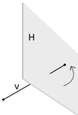
Fig. 1. A predicate of typeH

A. Collision predicates and spin-quadrics

Acollision predicate or shortly a predicatecan be inter-preted as a formula which yields different values for collision and no-collision arguments. A predicate induce an oriented surfacein a configuration space. Configurations that cause a collision, are on one side of the surface. On the other side, there are configurations that do not cause a collision. The surface is a set of configurations that ”touch” an obstacle, but not penetrate it. Combinatorial method involves consid-eration of a set of predicates, which are created from a scene. One of the first to use a term collision predicate was Canny [16]. A concept of a predicate is also known under different names, such as a ”contact” in [10] or a ”basic contact”, as in [17].

The following two basic predicates definitions are intro-duced:

Definition 1 (A half-space predicateH): Assume that U is a normal vector anddis a plane distance of a half-space H. LetV be a non-zero vector. The formula:

Hs(H, V) =Hs((U, d), V) =U·Rs(V) +d is called a half-space predicate.

The above formula evaluates a positive or negative value depending on whether the rotated vector v has it end on positive or negative side of half-plane. We assume that v’s begin lies at 0. A schematic view of Hpredicate is shown in figure 1.

Definition 2 (A screw predicateS): Assume that K and L are ends of a stationary segment and A and B are ends of a rotating segment. The formula:

Ss(K, L, A, B) =

(K×L)·R_{s(A−B) + (K−L)·}R_s(A×B)

is called a screw predicate.

The above formula evaluates a positive or negative value depending on whether rotating vector is oriented clockwise or counter-clockwise in respect to the stationary vector. A schematic view ofS predicate is shown in figure 2.

It can be shown that H and S are both special cases of a new predicateG. In result, only aG predicate needs to be considered.

Definition 3 (A general predicateG): Assume thatKand L are ends of a stationary segment and A and B are ends of a rotating segment andcis a scalar. The formula:

Gs(K, L, A, B, c) =

Fig. 2. A predicate of typeS

is called a general predicate.

The equivalence of H toG andS toG predicates is due to the following two remarks:

Remark 1 (HtoG predicate correspondence): A predi-cate H(U, d, V) is a special case of a predicate G(K, L, A, B, c)with the following parameters:

K = V ×R

L = V ×(V ×R)

A = U

B = −U

c = 2dkV ×Rk2

whereR is an arbitrary non-zero vector that is not parallel toV.

During our research we tried different methods for choos-ing aR vector. We selected few practical ones.

Remark 2 (S toG predicate correspondence):

Predicate S(K, L, A, B) is a special case of a predicate G(K, L, A, B, c)with the following setting:

c= 0

A genericGpredicate sets an oriented quadric (a quadratic surface) in configuration space. Moreover, the quadric is a quadratic form in spin-space, thus it will be henceforth called spin-quadric. In case of Spin(3)configuration space we have: Theorem 1: A spin-quadric for a given general predicate G is a quadratic form in Spin(3)and can be expressed by:

Gs=sTMGs

wheres= [s12, s23, s31, s0]T and MG’s elements are linear expressions of G’s parametersK,L,A,B andc.

We assume that collision algorithm should detect a col-lision of polyhedra borders. Without any loss, it can be assumed that all faces are triangles. Two polyhedra collide if and only if their borders intersect. This is realized by checking a collision between all pairs of triangles: one from the rotating polyhedron and other one from scene obstacles. By using some ideas from [18], we defined a predicate detecting a triangle-triangle collision.

Theorem 2 (A triangle-triangle predicateT T): A generic collision test between a stationary triangle KLM and a rotating triangle ABC can be expressed with 9 predicates of type S only. The characteristic matrix MT T is:

MT T = 



S(K, L, A, B) S(K, L, B, C) S(K, L, C, A)

S(L, M, A, B) S(L, M, B, C) S(L, M, C, A)

S(M, K, A, B) S(M, K, B, C) S(M, K, C, A)





The predicate evaluates collision if and only if there exist a row or a column in MT T that all it’s elements are of the same sign. Triangle-triangle predicate is denoted by T T(K, L, M, A, B, C).

Assume that T Ti

s, i = 1...nm are T T predicates of all triangle pairs for a given scene. The following formula is a predicate sentencefor a scene:

Sentences:=[

i

T Ti s

As a result of the this step, a list of quadrics is given. These quadrics introduce an arrangement in Spin(3). A predicate sentence, created from the scene, is also stored in order to be used later.

B. Spin-quadric intersection as graph edges

Computing an intersection of two spin-quadrics is not an easy task. It is not easy, even in a case of intersection of two quadratic surfaces in R3

. There exist algorithms that partially solve this problem. In particular, [19], [20] and [21] are known methods. Only recently, first complete implemen-tations of quadric intersection inR3

were developed: [22] and [23]. The case of an intersection, where the resulting curve is not singular, was solved first. A standard procedure is to follow a method proposed by Levin [24]. The problematic cases are those, involving singular intersections. Much work is needed to handle all specific cases, one by one. Currently, two implementations are available: QI library [23] (available online [25]) and Berberich’s implementation [22]. The first of these, return parametrization of resulting intersections. The latter does not. Both implementations present a similar performance. Although the dimensionality of Spin(3)andR3

is the same, both spaces posses a very different topology. One of the main results of this paper is to show that, a quadric intersection library for R3

can also be used to perform intersections in Spin(3).

Theorem 3: LetAbe an algorithm for quadric intersection inP3

(projective space). By usingAit is possible to easily construct an algorithm B which intersects a pair of spin-quadrics in Spin(3). The asymptotic complexity ofB is the same as the asymptotic complexity ofA.

The above theorem strictly depends on a fact, that library internally uses homogeneous coordinates, and that the result-ing intersection curve is near-optimally parametrized.

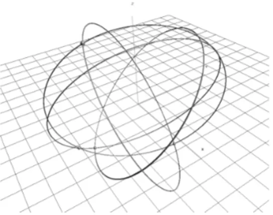
In spin configuration space, quadric intersection generates a curve which will be called as a spin-QSIC (spin quadric surface intersection curve) in contrast to QSIC (quadric surface intersection curve), as used in literature [26] and [27]. In the figure 3 we show an example projection of spin-QSIC curves ontoR3

. The projection is realized by dropping one of four spinor coefficients.

C. Spin-quadric and spin-QSIC intersection as a graph vertex

An important part of new algorithm is vertex construction. The number of possible vertices isO(n3

Fig. 3. An example set of spin-QSICs in Spin(3)

TABLE I

MOTION PLANNING ANDHEMMER ALGORITHM COMPARISION

Property Motion planning in SO(3) Hemmer

Topology Spin(3) R3

Dimension 4 3

Constraints 1 0

Objects quadrics in Spin(3) quadrics inR3

Running time O(n3

log(n)) O(n3

log(n))

method can be also applied to the case of spin-QSIC and spin-quadric intersections. As a result of intersection we get at most 8 vertices, given by parameter values on a parametrized spin-QSIC. Equations of degree at most 8, have to be solved. The result cannot be obtained in generic case, so the solutions are represented by non-overlapping intervals with a single polynomial root within. Hemmer used a classical real root isolation algorithm that subdivides consecutive intervals in search of zeroes (Vincent’s method). In our implementation a new recently implemented algorithm is used. It is an Akritas’ algorithm, which implementation comes from MATHEMAGIX [29] library (the ”realroot” module). Tests show that the latter implementation is about over a dozen times faster.

D. Graph optimization and final setup

As a result of construction of graph edges and vertices, some of these features can be doubled. These redundant features must be removed. This is achieved in the similar manner as described in [28]. Hemmer’s method utilized a floating interval arithmetic to avoid costly computations on exact numbers (provided by MPFI library [30]). We follow that method in our new algorithm. One of the improvements is our new method of fast determination of polynomial sign for a given point.

E. New algorithm in contrast to Hemmer’s algorithm

Hemmer [28] proposed a complete algorithm for comput-ing an intersection graph of quadrics in R3

. The algorithm also uses QI library for quadric intersection. There are few similarities and differences between these two algorithms, presented in table I. Note: n is a number of quadrics in an arrangement.

Some procedures, described in Hemmer algorithm exist in the new algorithm. Some of these were reimplemented

with new algorithm to improve overall performance. These include: an improved algorithm for polynomial root isolation and a method of determining a polynomial sign at given point.

F. Construction of a motion path

Given a preprocessed configuration space, it is possible to construct any number of motion paths. There are many ways to choose a motion path. A common solution is to choose any path, which is later ”optimized”. In out algorithm we choose a path along the edges of configuration space graph. This approach has an advantage that there is a parametrization given for each edge in the graph, which can also be a parametrization of the motion. Typically, a motion path can be optimized by shortening the path in the domain of free configuration space.

G. Adaptive computations in a space of rotations

One of the disadvantages of complete algorithms is a fact that many constructions could be avoided. The problem is even more serious because the complexity of generated con-figuration space is high. The proposed new algorithm relies on a adaptive computation method. The method is based on a generation of a random and approximate description of configuration space geometry. In most of cases such a description allows one to not compute the exact geometry of the whole configuration space.

An arrangement of quadrics in SO(3) induces a set of cells in that space. Each cell contains only points that are on the same side of all oriented quadrics. A sequence of signs is called acell coordinate. The length of a coordinate is usually denoted by l and it is equal to the number of quadrics. Both start and end configuration are contained in some cells (possibly different). If cells are considered as a vertices of a graph, their neighbourhood can be viewed as edges of the graph. Such graph will be calleda cell graph. An edge path in a cell graph is an approximate solution to a motion planning problem. A complete algorithm does utilize this information and constructs only the geometry that is related to all cells along the solution path in a cell graph. The difference between the approximate cell graph and complete cell graph is that in the first case the graph is only used as a localization method, not a target structure of the algorithm. The geometric part is a separate part of the whole algorithm, which in fact can work separately. It is also exact, while a cell graph is constructed in floating point arthimetic. Because of that, we would like that a cell graph is constructed quickly and to be a good quality. A cell graph of a good quality is a graph which is has the same topological properties as the whole configuration space. The number of graph components should be as close as the number of topological components in the complete configuration space.

Fig. 4. An example intersection of a circle of rotations with spin-quadrics

TABLE II

RUNNING TIMES OF CELL GRAPH CONSTRUCTION

no. samples no. different cells time

5000 2554 0.08 s

10000 5022 0.14 s 50000 24882 0.7 s 100000 48849 1.8 s 200000 93676 3.9 s 500000 218127 10.2 s

We introduced a new method. The idea is to pick a random 1-dimensional set of rotations (which forms a circle of rotations) and intersect it with all the quadrics. As a result we get a list of intersections given by an angle parameter on the intersecting circle. We sort the list and choose samples to be the middle points between consecutive parameter values. By using this method, no cells can be missed along the intersecting circle. An example is presented on 4. Intersecting circle is distinguished with a dotted line. The two black boxes are samples which would be chosen by our method. The method has many advantages. Firstly, it is very efficient - most of generated samples hit unique cells. Secondly, it guarantees that the generated set of cells is always connected. In fact, the method generates a complete loop in cell graph. It is not a trivial task to find out which cell pairs are neighbours. The number of cells in a typical situation is about few millions, while the coordinate length is few hundred bits. With some minor assumptions, it can be shown that two cells are neighbours if and only if their coordinates differ in only one bit at the same position. A naive Θ(n2

l) algorithm to compute cell neighbours is unacceptable. It is only usable for very small scenes.

A new algorithm for computing cell pairs was developed. It is optimal in asymptotic complexity, which is Θ(nl). The new algorithm allows one to achieve good quality cell graphs in acceptable times. A typical arrangement contains few hundreds of quadrics. Example running times for 175 quadrics are presented in table II. It can be observed that the running times are linear to the number of samples. For a given n samples, the algorithm is able to locate about

35−50% of ndifferent cells.

The implementation was tested on a Linux 3.2.0-1-amd64 SMP on a 2.40 GHz processor with 4 GB RAM.

H. Implementation

All presented results were implemented in author’s library libcs. The library is designed in a generic fashion, so the most of underlying algorithms are universal. The bottom layer of the library is CGAL [15] on top of which a spin kernel is introduced. Visualization application is also available, which can display configuration spaces with their contents.

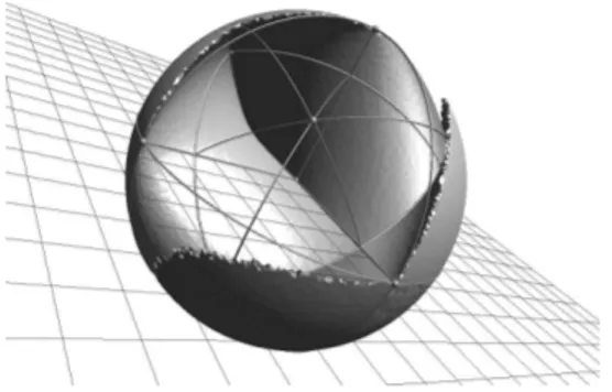
Fig. 5. An example projection of Spin(3)configuration space contents

I. Polyhedra with interior included

The presented algorithm detects only collisions based on border collisions. If required, it is possible to extend the algorithm to handle interior collisions as well. This can be achieved by adding a number of predicates of typeHto the predicate sentence. The idea of detecting a collision of two filled polyhedra comes from [17].

J. Localization

It is an open problem how to localize geometric computa-tions in non-Cartesian spaces. Especially interesting is how to avoid computation of the whole configuration space at once, and only compute its features on demand or incremen-tally. This subject and further generalizations are subject for author’s future research.

IV. CONCLUSION AND FUTURE WORK

We have shown that, by using some latest algorithms related to 3D arrangement of quadrics, we are able to implement an exact motion algorithm involving 3D rotations. Such an algorithm allows one to construct hybrid algorithms of a new class. It can also be a part of more complex algorithm for a motion planning with more than three degrees of freedom. It must be noted, that it is possible to extend the structure of the configuration space by introducing cells in the arrangement. There has already been some work done for arrangements of quadrics inR3

. Examples include [32] and [33]. An interesting and important problem, still under active research, is localization in the space of 3D rotations. These tasks are subject of author’s future work.

REFERENCES

[1] S. LaValle,Planning algorithms. Cambridge Univ Pr, 2006. [2] J.-C. Latombe,Robot motion planning. Springer Verlag, 1990. [3] M. Foskey, M. Garber, M. Lin, and D. Manocha, “A voronoi-based

hybrid motion planner,” in Intelligent Robots and Systems, 2001. Proceedings. 2001 IEEE/RSJ International Conference on, vol. 1. IEEE, 2001, pp. 55–60.

[4] S. Hirsch and D. Halperin, “Hybrid motion planning: Coordinating two discs moving among polygonal obstacles in the plane,”Algorithmic Foundations of Robotics V, pp. 239–256, 2004.

[5] D. Hsu, G. S´anchez-Ante, and Z. Sun, “Hybrid prm sampling with a cost-sensitive adaptive strategy,” inRobotics and Automation, 2005. ICRA 2005. Proceedings of the 2005 IEEE International Conference on. IEEE, 2005, pp. 3874–3880.

[6] L. Zhang, Y. Kim, and D. Manocha, “A hybrid approach for complete motion planning,” inIntelligent Robots and Systems, 2007. IROS 2007. IEEE/RSJ International Conference on. IEEE, 2007, pp. 7–14. [7] J. Lien, “Hybrid motion planning using minkowski sums,”Proceedings

[8] G. Vegter, “The visibility diagram: a data structure for visibility problems and motion planning,”SWAT 90, pp. 97–110, 1990. [9] P. Agarwal, B. Aronov, and M. Sharir, “Motion planning for a convex

polygon in a polygonal environment,” Discrete & Computational Geometry, vol. 22, no. 2, pp. 201–221, 1999.

[10] F. Avnaim, J. Boissonnat, and B. Faverjon, “A practical exact motion planning algorithm for polygonal objects amidst polygonal obstacles,” inRobotics and Automation, 1988. Proceedings., 1988 IEEE Interna-tional Conference on. IEEE, 1988, pp. 1656–1661.

[11] V. Koltun, “Pianos are not flat: Rigid motion planning in three dimensions,” inProceedings of the sixteenth annual ACM-SIAM sym-posium on Discrete algorithms. Society for Industrial and Applied Mathematics, 2005, pp. 505–514.

[12] L. Dorst and D. Fontijne,Geometric algebra for computer science: an object-oriented approach to geometry. Morgan Kaufmann, 2007. [13] P. Lounesto,Clifford algebras and spinors. Cambridge Univ Pr, 2001,

vol. 286.

[14] GMP - The GNU Multiple Precision Arithmetic Library. [Online]. Available: http://gmplib.org

[15] CGAL - Computational Geometry Algorithms Library. [Online]. Available: http://www.cgal.org

[16] J. Canny,The complexity of robot motion planning. The MIT Press, 1988.

[17] F. Thomas and C. Torras, “Interference detection between non-convex polyhedra revisited with a practical aim,” inRobotics and Automation, 1994. Proceedings., 1994 IEEE International Conference on. IEEE, 1994, pp. 587–594.

[18] O. Devillers, P. Guigue et al., “Faster triangle-triangle intersection tests,” 2002.

[19] L. Dupont, D. Lazard, S. Lazard, and S. Petitjean, “A new algorithm for the robust intersection of two general quadrics,” inProc. 19th Annu. ACM Sympos. Comput. Geom, 2003, pp. 246–255.

[20] Z. Xu, X. Wang, X. Chen, and J. Sun, “A robust algorithm for finding the real intersections of three quadric surfaces,” Computer aided geometric design, vol. 22, no. 6, pp. 515–530, 2005.

[21] B. Mourrain, J. T´ecourt, and M. Teillaud, “On the computation of an arrangement of quadrics in 3d,”Computational Geometry, vol. 30, no. 2, pp. 145–164, 2005.

[22] E. Berberich, M. Hemmer, L. Kettner, E. Sch¨omer, and N. Wolpert, “An exact, complete and efficient implementation for computing planar maps of quadric intersection curves,” inProceedings of the twenty-first annual symposium on Computational geometry. ACM, 2005, pp. 99– 106.

[23] S. Lazard, L. Pe˜naranda, and S. Petitjean, “Intersecting quadrics: An efficient and exact implementation,”Computational Geometry, vol. 35, no. 1-2, pp. 74–99, 2006.

[24] J. Levin, “A parametric algorithm for drawing pictures of solid objects composed of quadric surfaces.” Commun. ACM, vol. 19, no. 10, pp. 555–563, 1976. [Online]. Available: http: //dblp.uni-trier.de/db/journals/cacm/cacm19.html#Levin76

[25] QI - Quadric intersection. [Online]. Available: http://vegas.loria.fr/qi [26] C. Tu, W. Wang, and J. Wang, “Classifying the nonsingular intersection

curve of two quadric surfaces,” inGeometric Modeling and Processing, 2002. Proceedings. IEEE, 2002, pp. 23–32.

[27] W. Wang, B. Joe, and R. Goldman, “Computing quadric surface intersections based on an analysis of plane cubic curves,”Graphical Models, vol. 64, no. 6, pp. 335–367, 2002.

[28] M. Hemmer, L. Dupont, S. Petitjean, and E. Sch¨omer, “A complete, exact and efficient implementation for computing the edge-adjacency graph of an arrangement of quadrics.” J. Symb. Comput., vol. 46, no. 4, pp. 467–494, 2011. [Online]. Available: http://dblp.uni-trier.de/db/journals/jsc/jsc46.html#HemmerDPS11 [29] Mathemagix - A free computer algebra system. [Online]. Available:

http://mathemagix.org

[30] MPFI - Multiple Precision Floating-point Interval library. [Online]. Available: http://mpfi.gforge.inria.fr

[31] K. Shoemake, “Uniform random rotations,” in Graphics Gems III. Academic Press Professional, Inc., 1992, pp. 124–132.

[32] N. Geismann, M. Hemmer, and E. Sch¨omer, “Computing a 3-dimensional cell in an arrangement of quadrics: Exactly and actually!” inProceedings of the seventeenth annual symposium on Computational geometry. ACM, 2001, pp. 264–273.