Setembro, 2014
Diogo Manuel Pires de Matos
Licenciatura em Engenharia Informática
State Detection in a Financial Portfolio
Dissertação para obtenção do Grau de Mestre em Engenharia Informática
Orientador: Prof. Doutor Nuno Marques, Professor Auxiliar, FCT
A Self-organizing maps approach for financial time series
Presidente: Prof. Doutor Carlos Augusto Isaac Piló Viegas Damásio
Arguente: Prof. Doutora Maria Margarida Guerreiro Martins dos Santos Cardoso
States Detection in a Financial Portfolio
Copyright © Diogo Manuel Pires de Matos, Faculdade de Ciências e Tecnolo-gia, Universidade Nova de Lisboa.
This study analyses financial data using the result characterization of a self-organized neural network model. The goal was prototyping a tool that may help an economist or a market analyst to analyse stock market series. To reach this goal, the tool shows economic dependencies and statistics measures over stock market series.
The neural network SOM (self-organizing maps) model was used to ex-tract behavioural patterns of the data analysed. Based on this model, it was de-veloped an application to analyse financial data. This application uses a portfo-lio of correlated markets or inverse-correlated markets as input. After the anal-ysis with SOM, the result is represented by micro clusters that are organized by its behaviour tendency.
During the study appeared the need of a better analysis for SOM algo-rithm results. This problem was solved with a cluster solution technique, which groups the micro clusters from SOM U-Matrix analyses.
The study showed that the correlation and inverse-correlation markets projects multiple clusters of data. These clusters represent multiple trend states that may be useful for technical professionals.
Keywords: Financial Markets, SOM, Correlated Markets, Clustering over
Este estudo analisa a caracterização de dados financeiros que é feita através de um modelo de rede neural auto-organizada. O objetivo foi a criação de um pro-tótipo que tem como funcionalidade ajudar um economista ou analista de mer-cado. Para alcançar este objetivo, a ferramenta mostra as dependências e estatís-ticas económicas que foram calculadas apartir de séries financeiras.
O modelo de rede neural SOM (mapas auto-organizáveis) foi usado para extrair padrões de comportamento dos dados analisados. Tendo por base esse modelo, foi desenvolvida uma aplicação que permite analisar dados financei-ros. Esta aplicação utiliza um portfolio de mercados correlacionados ou merca-dos inversamente correlacionamerca-dos como entrada. Após a análise com SOM, o resultado é representado por micro grupos que estão organizados pela sua ten-dência comportamental.
Durante o estudo surgiu da necessidade de melhorar a análise resultante do algoritmo SOM. Este problema foi resolvido com uma técnica de agrupa-mento, que agrupa os micro estados representados na U-Matrix do SOM.
O estudo mostrou que os mercados correlacionados e inversamente corre-lacionados projetam vários grupos de dados. Estes grupos organizam-se por tendencia podendo ser uma analise importante para os profissionais técnicos.
Palavras-chave: Mercados Financeiros, SOM, Mercados Correlacionados,
1 INTRODUCTION ... I
MOTIVATION ... II
1.1
OBJECTIVES ... II
1.2
1.2.1 Data Selection ... ii
1.2.2 Characterizations and first usage of SOM ... iii
1.2.3 Behaviour and Time Series Generator ... iii
THESIS STRUCTURE ... III 1.3 2 RELATED WORK ...V FINANCIAL MARKETS STUDIES ... V 2.1 2.1.1 Portfolio selection ... vi
2.1.2 Correlation in markets ... vi
2.1.3 Moving Average ... vii
2.1.4 Hurst ... ix
CLUSTERING ... XII 2.2 2.2.1 K-means ... xii
2.2.2 KNN ... xiii
2.2.3 SOM ... xiii
CHARACTERIZING THE CLUSTERING ... XIX 2.3 2.3.1 Flooding... xix
2.3.2 Methods for evaluating clustering quality ... xix
2.3.3 Generator ... xxi
3 PROPOSED APPROACH ... XXIV ARCHITECTURE ... XXV 3.1 3.1.1 General Architecture ... xxv
8
SOURCE DATA ... XXVII
3.2
CHARACTERIZATION METHOD -MIN-MAX NORMALIZATION ... XXVIII
3.3
STATE IDENTIFIER /CLUSTERING ... XXIX
3.4
3.4.1 Local Min... xxix 3.4.2 Flood Algorithm ... xxxi 3.4.3 Missing Classification Procedure ... xxxii
STUDY OF THE GENERATED STATES ... XXXIV
3.5
3.5.1 State relevance of the data set. ... xxxiv 3.5.2 Graph transition measures ... xxxv 3.5.3 Centroids distances measures ... xxxvi
GENERATOR ... XXXVII
3.6
4 CLUSTERING TECHNIQUE VALIDATION ... XXXIX
WINE DATA SET ... XL
4.1
IRIS DATASET ... XLII
4.2
SYNTHETIC TIME SERIES ... XLIV
4.3
5 APPLICATION TO FINANCIAL DATA ... XLVII
CORRELATION METHOD ... XLVIII
5.1
CASE STUDY ONE ... XLVIII
5.2
INVERSE-CORRELATION METHOD ... LIII
5.3
CASE STUDY TWO ... LIII
5.4
6 CONCLUSIONS ... LIX
FUTURE WORK ... LX
6.1
9
Figure List
10
11
Tables List
1
Introduction
Financial markets may be subjected to extreme and complex events, which can easily go unnoticed by human perception. Many research groups search new algorithms and new technology that allows the extraction of knowledge from several conjoint data streams. In this thesis we study several methods that may be useful for developing new ways to analyse and visualize financial markets.
This study is organized in three major phases that can be titled as data characterization, state detection and validation. The data characterizations fo-cus on choosing a set of time series and also prepare the data for the state detec-tion. The state detection is based on the use of SOM (self-organizing map) [1] to find similarity patterns in the stream data. Finally, the validation phase consists of proposed tools to analyse the studied model.
SOM gives the possibility to use the properties of a neuronal network that self-organizes the characterized data. This technique presents data in a two di-mensional map organized by its characteristics. We study how this method can be used to know how the financial markets are correlated, which is an added value to technical analysis studies. Possible applications of this method are the study of global inter-dependencies presented. Also, this study lead to develop a new method for discriminating clusters in SOM.
2
Motivation
1.1
The financial markets data may be one of the most complex fields of analysis. The speculation and the competition in stock markets may lead to high volatili-ty and investment risk that could be mitigated if an early detection of relevant patterns is available. For example, this can be used to guide regulatory policies.
The problem addressed is the difficulty in mapping the state of the finan-cial system. Based on this principle, mapping the huge number of states of a fi-nancial system seems a difficulty that stands out, as well the detection of inter-actions between the markets. Therefore the sub-problem of mapping interac-tions of correlated markets states is relevant. This study will take in considera-tion how the correlated markets interact when the global systems changes and if this sub-problem addresses any type of micro states that can be a marker of upcoming crises states or the return to normality after a crisis state.
The algorithm of self-organizing maps appears to be a good method for this problem. It is a self-adapting neuronal network that has the particularity of identifying clusters in data and also project them in a two dimensional map. This algorithm is already being used to study financial data but many ap-proaches are still unexplored.
Objectives
1.2
The main objective for this thesis is to understand how correlation between markets may help to identify particular trend change states. As mentioned be-fore the chosen algorithm was SOM (self-organizing maps). The objective is to cluster the data by a state of behaviour after training the net and finally define a path of states (clusters) which have been visited.
1.2.1 Data Selection
3
results and decide if correlation of stocks brings a useful analysis to stock mar-ket traders.
1.2.2 Characterizations and first usage of SOM
The second sub-goal for this thesis is characterize the data selected in the previ-ous goal. This process uses SOM algorithm.
After the data was treated, it was classified with the SOM algorithm. This classification will be filtered by other clustering processes that uses the SOM distances matrix (UMAT). This process will allow the formation of big clusters that gather closer neurons in the map.
1.2.3 Behaviour and Time Series Generator
Based in this sub–goal several visual tools will be tested as possible new ways for analysing the states of the time series.
A particularly interesting visualization tool will be proposed by generat-ing a time series based on the obtained clusters. The new time series will be an-alysed and compared with reality time series.
With this simulation it will be possible to see the stability of different time periods. Each state will present different mean and variance according to the considered cluster. It is expected that during a crises period the variance will be bigger than during a stable period.
Thesis Structure
1.3
Chapter 2 consists on the results of the literature studied where the support for the thesis is presented. There is a brief overview about financial studies, cluster-ing algorithms and some methods to analyse the clustercluster-ing.
In Chapter 3 we can find the proposed approach for this system. This part is divided in the Architecture of the system, the data source, the characteri-zation method, the state identifier/clustering, the studies of the general states and the generator.
4
Chapter 5 tests the algorithm with the financial data. This chapter is di-vided in 3 sections. The first two corresponds to testing the case studies and the last on corresponds to presented some future work that may be done
2
Related Work
Financial Markets Studies
2.1
Financial market studies can be divided in two areas namely technical and fundamental analyses. These studies have the objective of understanding the stock market movements, and ideally characterizing the economy. Here we aim to study possible tools to identify decision patterns that help in the generation of profitable processes in stock market exchange. The possibility of profitability attracts many people that are committed to improve the returns of their invest-ments and this can be related with the efficient market approach of [2].
Fundamental analysis can be defined as a method of evaluating an intrin-sic value of a security by examining related economic, financial and other quali-tative and quantiquali-tative factors. This science also attempts to study everything that can affect the securities value, including macroeconomic factors (like the overall economy and industry conditions) and company-specific factors (like financial condition and management) [3].
Technical analysis is defined [3], as the academic study of historical chart patterns and trends of publicly traded stocks. Much of the fundamental analysis and market opinions may be reflected in the stock price that by getting the re-current price patterns and fitting them to past movement, may be possible to predict the future of the price.
6
2.1.1 Portfolio selection
Portfolio investment is one form to do investment with low risk value when compared with single stock investment. One well known study [4] presented a statistic process to select some stocks evaluations from securities that are low correlated. Based in the rule which implies both that the investor should diver-sify and that he should maximize expected return. The rule states that the in-vestor does (or should) diversify his funds among all those securities which give maximum expected return.
A study [5] explains the analyses to predict the future and understand the past. By risk measures it may be constructed a portfolio to maximize the returns of a found.
2.1.2 Correlation in markets
The effect of correlated markets in the global economy has been object of study. As showed in [6] reveals that crises states contagion between different countries is actually a fact. It has been used a correlation coefficient between ri and rjthat can be written as:
ρ = Cov(ri, rj) √Var(ri) × Var(rj)
(1)
This calculus is actually called Pearson's correlation coefficient. It oscil-lates between -1 and +1. Positive means that the two series are correlated and negative that they are not correlated. The value 1 means that is considered a perfect positive correlation but that value is very rare.
7
As was showed in the study of local correlation Person coefficient pre-sented the addressed problems, and the proposed approach seem to be a lot stable in an exchange rates dataset. This result may be seen in the figure 1.
Figure 1 - Local correlation scores [7]
This study was made to select the datasets used by the SOM algorithm. The data selected for a set of stocks should be the most correlated. By doing this we can nominate the data as a set of correlated markets, which can be used for state detection process using a cluster technique.
In the next section it will be analysed how some technical indicators that were studied with the objective of characterizing a stock action time series. The ones that have been analysed were the moving average and the Hurst index.
2.1.3 Moving Average
8
The formula used to calculate the moving average uses 𝑡 that represents the given time and the k represents the period of the moving average. With this we have:
mavg(t)=∑ xt t
t=t−k
k (2)
In [8] is showed the use of moving average in constructing a profitable process. It is also explained some proprieties of using different time length with different moving averages. In the figure below can be seen two moving average calculations. One is up to 25 days period and the other is up to 40 days period. Analysing the figure 2 we can check that the index shows a more stable line compared to the real time series. This makes a lot easier to analyse the trend of the time series.
Figure 2 - Moving Average [8]
This technical indicator may be combined with machine learning tech-nique to make a profitable process. In the study[9]is used a neuronal network to generate data and illustrate the potentiality as a trader method based on the Eurostoxx50 financial time series.
9
problem in hand. Choosing the period with no specialist knowledge, may lead to a bad performance analyses.
2.1.4 Hurst
Hurst exponent [10] can be used as a long memory process for capital markets, making it one of the topics in finance.
The Hurst exponent referenced in [11], was used for fractal analysis but has been explored to use in many other research fields, including economics. This calculus has provided a measure for long term memory and the fractality of a time series. It is also known that Hurst exponent varies between 0 and 1, which can be considered in three subsets:
𝐻 = 0.5 indicates a random series
0 < H < 0.5 indicates an anti-persistent series
0.5 < 𝐻 < 1 indicates a persistent series
Working with this index could be a good answer to measure time series predictability. It also can be used to measure the comparison of a generated time series with the real series that makes this index as an added value for the study.
Hurst exponent calculation
To calculate the Hurst exponent, the first action has to be the range estimation on the time span of 𝑛 observations. A time series of full length 𝑁 is divided into a number of shorter time series of length 𝑛 = 𝑁, 𝑁/2, 𝑁/4, ... The average re-scaled range is then calculated for each value of 𝑛.
For a (partial) time series of length 𝑛, 𝑋 = 𝑋1, 𝑋2 , … , 𝑋𝑛, the rescaled range is calculated as follows:
Calculate mean value m:
m = 1n ∑ Xi n
i=1
(3) Calculate mean adjusted series Y:
10 Zt = ∑ Yi
t
i=1
, t = 1, 2, … , n (5)
Calculate range series R:
Rt = max(Z1, Z2, … , Zt) – min(Z1, Z2, … , Zt)
t = 1, 2, … , n (6)
Calculate standard deviation series S:
St = √1t ∑(Xi− u)2 t
i=1
, t = 1, 2, … , n (7)
Calculate rescaled range series (R/S):
(RS) t =RtSt t = 1, 2, … , n (8) Hurst found that (R/S) scales by power-law as time increases, which indicates:
(RS) t = c × tH (9)
11
Figure 3 - Hurst Index [12]
12
Clustering
2.2
In this research appears the need of studying some methods that may be used to correlate and classify certain patterns of crisis state. As result some IA algo-rithms have been studied but by general characteristics self-organizing maps was chosen.
2.2.1 K-means
The k-means algorithm is a clustering algorithm widely known and used as presented in [13]. The principal objective of the algorithm is to distribute the da-ta by a given number of clusters. By this we have the set of 𝐾 that represent the number of clusters. The 𝐾 setting may be considered as problem when the number of data classes/clusters is unknown. This problem has already some solutions for the k number auto-detection (a review of k-mean for k detection may be found in [14]).
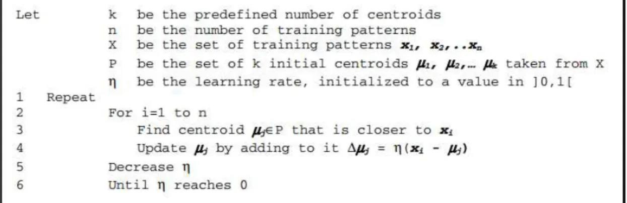
After defining the number k, it also has to be defined the first k centroids that will be used in the learning process. The learning procedure is used to up-date the cords of each k centroids for a better cluster representation. This pro-cedure uses a group of training patterns, which are sets of data to represent each cluster. The original algorithm [15] is depicted in figure 4:
Figure 4 - K-means training process
After training, the data k-means uses an activation function for giving the respective centroid for each data object. If we have a data set 𝑋 = (𝑥1, 𝑥2, … , 𝑥𝑛), k-means will classify which object 𝑥𝑖 as a cluster 𝑐𝑖, where k is
13 𝑎𝑟𝑔
𝐶 𝑚𝑖𝑛 ∑ ∑ ‖𝑥𝑗 − 𝜇𝑖‖2 𝑥𝑖∈𝑆𝑖
𝑘
𝑖=1
(10)
, where 𝜇𝑖 is the centroid of cluster i.
2.2.2 KNN
The KNN algorithm [16] is a pattern recognition method used for classification and regression. This algorithm uses one simple way for its proposed objectives, where the objects are classified by majority vote of its neighbours. The majority class from the neighbours will be associated to the objects being classified.
The algorithm is executed based on labeled training samples, and also a configurable parameter k value. The value k may be defined by the user or au-tomatically generated through other techniques, in order to optimize the pro-cess (see also [17] that compares some improves in KNN algorithm). During the classification stage, the algorithm searches for the k closest neighbours of the object in the training dataset and chooses the label of the majority class.
The usual distances metrics used to determine the distance of one testing entity and one trained entity differs from the type of the variables. Usually for continuous variables is used the Euclidian distance and for discrete varia-bles may be used the Hamming distance. There are some studies [18] [19] to op-timize the distance metrics with some statistical algorithms. This may improve the classification accuracy.
2.2.3 SOM
The Self-Organizing Map, developed by Teuvo Kohonen in the 80’s [1], is a ma-chine learning algorithm that helps to characterize high-dimensional data set. This method uses an unsupervised learning to produce a low-dimension data set, discretized representation of the input space of the training samples, called a map.
14
usually 1 or 2 dimensional. The basic SOM training algorithm can be described as follows, referenced from [20]:
Variables and formulas 𝒔 current iteration 𝒍𝒊𝒎 iteration limit
𝒕 index of the input data vector in the input data set D
𝑫(𝒕) target input data vector
𝒗 index id the node in the map 𝑾𝒗 current weight vector of node v
𝒖 index of the best matching unit (BMU) in the map
𝞠(𝒖, 𝒗, 𝒔) restraint due to distance from BMU, usually called the neighbourhood function
𝜶(𝒔) learning restraint due to iteration progress
𝒅(𝒑, 𝒒) = √∑ (𝒒𝒏 𝒊− 𝒑𝒊)
𝒊=𝟏 Euclidean distance
𝑼𝒑𝑾𝒗(𝒔 + 𝟏) = 𝑾𝒗(𝒔) + 𝞠(𝒖, 𝒗, 𝒔) × 𝜶(𝒔) × (𝑫(𝒕) − 𝑾𝒗(𝒔) )
Update formula for BMU (Best Matching Unit), new weight
The SOM algorithm implementation:
This algorithm has the following steps, referenced in ref: [21]:
1) Randomize the map nodes weight vectors (𝑾𝒗)
2) Grab an input vector
3) Iterate each node in the map:
- Use the Euclidean distance (in 𝒅(𝒑, 𝒒)) formula to find the similarity between the in-put vector and the map nodes weight vector
- Track the node that produces the smallest distance (this node is the best matching unit, BMU)
4) Update the nodes in the neighbourhood of the BMU (including the BMU itself) by pulling them closer to the input vector. Use formula 𝑼𝒑𝑾𝒗(𝒔 + 𝟏)
5) Increase 𝒔 and repeat from step 2, until reach iteration limit (𝒍𝒊𝒎)
15
Figure 5 illustrates the training process evolution. It is possible to observe the selection of the best matching unit in the first step of the algorithm. The second step corresponds to update the best matching unit weight and also the surrounding neurons, as referenced in the formula 𝑼𝒑𝑾𝒗. Finally when the method achieves 𝒍𝒊𝒎, the map covers most of the input data.
Figure 5 - Training Process of Self-Organizing Map [20]
16
Figure 6 - Self-organizing map structure, referenced from [21]
There are some techniques for the interpretation of the map produced, a well-known is the UMatrix [22]. This technique provides us a simple way to visualize cluster boundaries in the map. This method is useful because it can find clusters in the input data without having any a priori information about the clusters. Figure 7 is an example of an UMatrix, in which darker colours repre-sent a larger distance between neurons and lighter colours reprerepre-sent low dis-tance between neurons.
Figure 7 – UMatrix, referenced from [23]
17
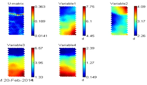
Figure 8 : Iris Dataset, generated in SOM toolbox
Figure 8 shows the importance of variable2 (corresponding to sepal width of iris dataset) on the identification of the upper cluster, which is classified as Iris-Setosa class. Also it can be seen the importance of the variable4 (Petal Width) in the identification of Versicolor class that can be easily mistaken with Iris-Virginica.
Some solutions were studied motivated by clustering on the UMAT. A two stage clustering approaches [24] seem to solve the clustering problem over the UMAT. The goal of a 2-stage clustering method is to overcome the major problems of the conventional methods as the sensibility to initial prototypes (proto-cluster) and the difficulty of determining the number of clusters ex-pected. The aim of the SOM at the first stage is to identify the number of clus-ters and relative centroids, to overcome, the problems described above. In the second stage, a partitioned clustering method will assign each pattern to the de-finitive cluster.
18
There are three post-processing methods that are known as a solution. The first one is the classic K-Means algorithm [25], which belongs to class of parti-tioned clustering methods. The second is the U-Matrix with connected compo-nents [26], a hierarchical algorithm with bottom-up approach. The third one is a model created by DAME group, inspirited by an agglomerative method based on dynamics SOM, hereinafter defined as Two Winners Linkage [27].
Just like a solution found in [28] that is based in [29] uses the property of high density region that is separated from another high density regions by re-gions of low density. Also this approach determines the number of clusters au-tomatically.
There are several studies that apply the SOM algorithm to finance. The first example represents an application of SOM algorithm for crises states detec-tion. This study [30] uses the self-organizing maps for mapping the state of the financial stability and as well for predicting systematic financial crises. The SOM algorithm was used to monitor the macro-financial vulnerabilities by lo-cating a country in a financial stability cycle, which is represented by the pre-crises, pre-crises, post-crises and tranquil state.
A recent work [31] explores this technique using the application of the SOM algorithm to characterise one stock market series based in some technical indicators. This approach gives some good results and there were some tech-nical indicators highlighted from the study. The best techtech-nical indicators were the volume, mean volume and the price variation. In the end, the SOM was able to identify some crises and stable states.
19
Characterizing the Clustering
2.3
2.3.1 Flooding
The Flooding is a concept that has been approached by some computer science algorithms. It extends from computer science network algorithms to graphics algorithms. For the network area we have the routing algorithm [33], which de-livered packets are send using flooding concept (the packet received is re-sent for all output link except to the source link).
Since the distance matrix of self-organizing map may be seen as a topo-graphic landscape, the flooding algorithm flood fill [34] was considered rele-vant to this study. This technique is used in the "bucket" fill tool of paint pro-grams to fill connected, similarly coloured areas with a different colour. This approach served as an inspiration for our approach that starts flooding from the local mins detected from the previous method of the clustering algorithm used in this study. A similar approach was used to identify clusters in the UMAT.
2.3.2 Methods for evaluating clustering quality
For knowing which was the best flood parameter some clustering quality measuring approaches were covered by the study. The SOM Topographic error and Quantization error [24] were the typically measures used to evaluate a map quality and may not be the best response to measure a second stage clustering result.
The study [35] compares some of the well-known cluster criterion measures for determining the number of clusters based in the clustering quali-ty. So this paper compares the stability measures of a recently proposed study [35], which also analyses the Calinski-Harabasz index [36] and the Krzanowski and Lai index [37].
As the Calinski-Harabasz index will be assumed as the variance ratio cri-terion (𝑉𝑅𝐶𝑘) defined as:
𝑉𝑅𝐶𝑘 =𝑆𝑆𝑆𝑆𝐵 𝑊×
(𝑁 − 𝑘)
20
, where SSB is the overall between-cluster variance, SSW is the overall within-cluster variance, k is the number of within-clusters, and N is the number of observa-tions.
The overall between-cluster variance SSB is defined as: 𝑆𝑆 𝐵 = ∑ 𝑛𝑖 ‖𝑚𝑖− 𝑚‖2
𝑘
𝑖=1
(12)
, where k is the number of clusters, 𝑛𝑖 is the number of observations by cluster, 𝑚𝑖 is the centroid of cluster i, and 𝑚 is the overall mean of the sample data.
The overall within-cluster variance SSW is defined as: 𝑆𝑆𝑤 = ∑ ∑‖𝑥 − 𝑚𝑖‖2
𝑥∈𝑐𝑖
𝑘
𝑖=1
(13)
, where k is the number of clusters, x is a data point, 𝑐𝑖 is the 𝑖𝑡ℎ cluster, and 𝑚𝑖 is the centroid of cluster 𝑖.
Well-defined clusters have a large between-cluster variance (𝑆𝑆𝐵) and a small within-cluster variance (𝑆𝑆𝑊). A larger 𝑉𝑅𝐶𝑘 ratio results in a better data partition. To determine the optimal number of clusters, maximize 𝑉𝑅𝐶𝑘 with respect to k. The optimal number of clusters is the solution with the highest Ca-linski-Harabasz index value.
As the Krzanowski -Lai index will be assumed as the variance ratio criterion (𝑉𝑅𝐶𝑘) defined as:
𝑉𝑅𝐶𝑘= |𝐷𝐼𝐹𝐹(𝑘 + 1)|𝐷𝐼𝐹𝐹(𝑘) (14)
, k represents the number of clusters and the 𝐷𝐼𝐹𝐹𝑘 is represented by:
DIFF(k) = (k − 1)2p× SSw(k − 1) − k2p× SSw(k) (15)
, where the SSw function represents the within-cluster variance (16).
21
from centroids. In analogy to Halkidi etal. [39] an instance of their index DB(K) may be defined as follows:
DB(K) = K ∑ R1 k K
k=1
for K ∈ ℕ (17)
, where
Rk = j = 1, … , K , j ≠ k (max Skd+ Sj
k,j ) for k ∈ [1, … , K] (18)
, and
Sk=∑ w1 k,i N
i=1 ∑ Wk,i‖xi− x̅k‖ N
i=1
for k ∈ [1, … , K] (19)
, as well as
dk,j = ‖x̅k− x̅i ‖ (20)
For each cluster 𝐶𝑘 an utmost similar cluster-regarding their intra-cluster error sum of squares-is searched, leading to 𝑅𝑘. Then the index calculates the average over these values. In contrast to the aforementioned cluster indexes, here, the minimal observed index indicates the best cluster solution.
2.3.3 Generator
The Monte Carlo method [40] relies on repeated random sampling to obtain numerical results. By running simulations many times in order to calculate those same probabilities heuristically just like actually playing and recording your results in a real casino situation: hence the name. They are often used in physical and mathematical problems and are most suited to be applied when it is impossible to obtain a closed-form expression or infeasible to apply a deterministic algorithm. Monte Carlo methods are mainly used in three dis-tinct problems: optimization, numerical integration and generation of samples from a probability distribution.
22
random value. The result of the model is recorded, and the process is repeated. A typical Monte Carlo simulation calculates the model hundreds or thousands of times, each time using different randomly-selected values.
When the simulation is complete, we have a large number of results from the model, each based on random input values. These results are used to de-scribe the likelihood, or probability, of reaching various results in the model.
There are several approaches to generate more elaborated models of a given phenomenon. For example in financial markets, Quasi-Monte Carlo [42] is a new adaption that can get better performance than Monte Carlo. The con-ventional Monte Carlo uses pseudo random values to evaluate an expression. This method yields an error bound that is probabilistic creating a disadvantage. Other disadvantage is that many simulations require a high level of accuracy, and this is something that the conventional method can’t promise.
Quasi-Monte Carlo is based in semi-deterministic instead of random se-quences. The basic idea of quasi-Monte Carlo is to use a set of points that are carefully selected in a deterministic fashion.
We call these numbers quasi-random even though they are perfectly de-terministic and have no random component.
In [43] QMC methods were used for estimating the value of a financial contract, such as an option, whose underlying assent fallow Black-Scholes mod-el. The goal is to estimate:
μ = E(gp(S1, … , St)) (21)
, where S1, … , St are price. The function gp is assumed to be square-integrable and it represents the discounted payoff the contract, and p is a vector of parameters (containing the risk-free rate r, the volatility σ, the strike price K, expiration time T, etc). The MC estimator would be:
Qn = 1n ∑ fp(ui) n−1
i=0
23
To have the QMC estimator it is just needed to use a randomized QMC point set. So the ui came from a randomized QMC point set, but being present-ed in the uniform distribution as MC. The only difference with MC is that with QMC, the observations fp(u0), … , fp(un−1) are correlated instead of being inde-pendent. With a carefully chosen QMC point set, the induced correlation should be such that the estimator has a smaller variance than the MC estimator.
Below is a figure of the results of comparing the Monte Carlo and the Quasi-Monte Carlo, where can be seen a faster convergence with the new method.
3
Proposed Approach
The architecture and the procedures will be presented in this section. The work was developed on matlab, which is capable of producing useful statistical measures and visualisation tools. With the integration of SOM Toolbox [44], a library that represents an implementation of the SOM algorithm, it was possible to program with a graphic and calculus tool which uses the self-organizing maps model. This library is composed by tools to generate many SOM model statistics interpretation, as an example, the UMAT view.
It was also added a module to flooding analyse the UMAT result. This module produces some visual and text files results that bring a new way of showing the results of SOM algorithm.
25
Architecture
3.1
3.1.1 General Architecture
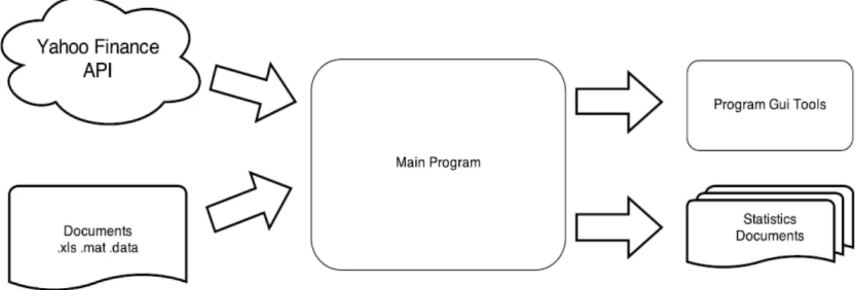
The proposed architecture, illustrated in figure 9, can be defined as a 3 stage system: the input layer, the main program and the output layer
Figure 10 - Proposed Architecture
The input layer uses the Yahoo Finance API and also the Documents of type .xls, .mat and .data (these documents should be formatted by the program protocol). The main program layer corresponds to the Main Program compo-nent of the figure, which defines the algorithms and calculus researched in this thesis. Finally the output layer that is defined in the figure 9 as the Program GUI Tools and Statistics files.
26
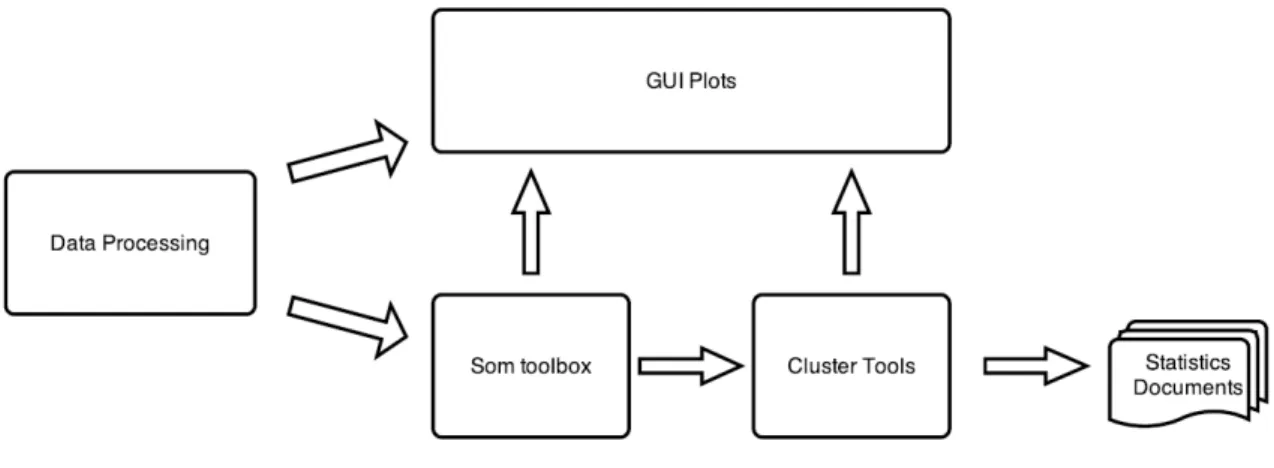
3.1.2 Work Flow Model
For a better understanding of the program concept, the figure 10 illustrates the work flow model. The work flow consists of various steps that the program has to process before achieving the final results, those were the statistic files pro-duced or the plots that the visual tools generated.
Figure 11 – Program Workflow
As it can be seen in the figure 9 the system starts by processing the input data. The input data comes from Yahoo services or from an input file. The data has to be distributed by the program global variables, to allow the GUI Plots tools be able to report statists graphics. If the next step is the usage of the SOM algorithm, the data has to be normalized before.
The SOM Toolbox corresponds to the SOM toolbox library. In this compo-nent we use the API of this library to generate the visual tools that will be showed in the GUI Plots component. We may stop the process right here or we may continue for the clustering tools.
27
Source Data
3.2
Most of the data comes from the Yahoo Finance Cloud System. This system is commonly used by investors and offers a free use of their API [45]. With this, it was possible to get a stock evaluation with detailed information about the price.
The Yahoo Finance System is limited by a thousand queries per stock ac-tion, but it hasn’t limitations with the size of the data. The connection that sends the data uses a stream channel that can be read to a variable in the code. This part of the code is done by the function get_hist_stock_data.m where the java.io library is used.
The query used asks for the high, low, open, close, volume of a stock daily value. It also has to be given the initial and final year date of the period to be analysed to process the query. In the study, the close value of the stock was used, that is the last value for the day in question.
Another way of adding data to the system is the use of default scripts cre-ated during the thesis elaboration or by using a file with the correct input for-mat. The default scripts of the thesis use data from the Yahoo cloud services but data is uploaded to a file, it allows any other provider to be used but still has to be with the correct format to allow the program to read it.
So to use the data from a file, the data must be structured by the following specifications:
1) The top of the columns should have the name of the companies or the name
of the calculus;
2) Each line of the file has to have the value for each variable
3) The first column is reserved to the date. The plots that show the date are
pro-gramed to work with days by line and the date should be in the format:
28
Characterization Method - Min-Max Normalization
3.3
Given a time window of 𝑛 days and an array of values 𝑎𝑟𝑟 we have 𝑛𝑜𝑟𝑚𝑎𝑙𝑖𝑧𝑒𝐵𝑦𝑀𝑖𝑛𝑀𝑎𝑥(𝑗):
𝑛𝑜𝑟𝑚𝑎𝑙𝑖𝑧𝑒𝐵𝑦𝑀𝑖𝑛𝑀𝑎𝑥(𝑗) = arr(j) − min (𝑎𝑟𝑟(𝑗 − 𝑛, … , 𝑗))
max(𝑎𝑟𝑟(𝑗 − 𝑛, … , 𝑗)) − min (𝑎𝑟𝑟(𝑗 − 𝑛, … , 𝑗))
So it has to calculate the minimum and maximum value of the subset of the array with length n. With these results it is calculated the subtraction of the position j value by the minimum of the subset array and also the subtraction of the maximum value calculated by the minimum value. With the previous two results, we divided the first result by the second result.
29
State Identifier / Clustering
3.4
The chosen technique to classify the states of the stock market time series was the SOM algorithm. Based on this, we started to classify the first testing data set and it was noticed that the information by BMU didn’t generate stable states with enough points. By analysing the trajectory over the UMAT it was noticed that some neurons should be considered as one. The result of these analyses leads the thesis to study a clustering algorithm that groups these sets of neu-rons.
To find the clusters in the UMAT it was used a two process procedure. The first procedure was to find interesting zones in the map that may represent a cluster, and the second was to explore those zones in order to decide which neurons may also be considered as the same cluster. For the first process we used the local min criterion and for the second process we used the flood fill algorithm.
3.4.1 Local Min
The local min is seen as a mathematic representation of a minimum for a certain set of a function. The local min can also be the minimum of the function but for that it has also to satisfy the global min restriction. The global restriction for a point x is:
𝑖𝑓 𝑓(𝑥∗) ≤ 𝑓(𝑥)𝑓𝑜𝑟 𝑎𝑙𝑙 𝑥 𝑖𝑛 𝑋
In the case we want the restriction for the local min value, it is needed to con-sider the X a sub set function.
Local min was important for this study because it is a way of studying the minimal points in a sub set. This type of technique is also used in some cluster-ing algorithms referenced in [46]. This has a particular interest for the study when the finding of some points of minimal distance is required, meaning points of high proximity values. The proximity is one of the clusters formation criterions.
30
minimal distance could be seen as the middle point of a cluster and by detect-ing all local min of a U-matrix we can have the maximum number of clusters considered by the distance between the entities. The density analysis has an important role in clustering but not for this study. The U-matrix represents only a distance matrix which doesn’t take in consideration the information about the density of samples by neurons.
To get the local min of the U-matrix we have to consider all the positions of the UMAT. For this we will test each position of the U-matrix to see if it is a minimum. If it is a minimum we mark that position with true value and if not we mark it with false value. We called this procedure in processMinimos fuction:
function [ minimalMat ] = processMinimos( Umat )
for x : allPositions(Umat)
if(isLocalMin(x, Umat)
minimalMat[x] = true;
else
minimalMat[x] = false;
end
end
end
To see if a position in the U-matrix is a local min, the position has to be compared with all its neighbours. If the position value is minimal comparing to its neighbours, it is returned the true value for this position, otherwise, it will be returned the false value. So for this we have Minimo with the minimum position and Mat with the U-matrix.
function [ bool ] = isLocalMin(Minimo, Mat)
for x : getNeighbours(Minimo, Mat)
if( Mat[Minimo] < Mat[x])
counter++;
end
end
if(counter == nuberOfNeighbours) bool = true;
else bool = false;
end
31
The neighbouring function varies with the topology of the map. The study used the hexagonal topology. So for this the number of neighbours was six. This may vary but the getNeighbours fuction was only programed for this type of topology that was the only one used in this study.
3.4.2 Flood Algorithm
The flood algorithm is used to join the entities or clusters in one entity. This algorithm is executed with the result of the local min algorithm, so the starting points to make the flooding are localMins found before. The flood will be executed to a limit that corresponds to the boundaries defined by the user. In the pseudo code of the algorithm, showed in the box, corresponds to the mean distance of the U-matrix.
function [ finalClusters ] = flood( localMins )
allClusters = LocalMins;
finalClusters = [];
meanValueUmat = mean(mean(Umat));
for cluster : allClusters
cluster = floodACluster(cluster, meanValueUmat );
addCluster(finalClusters,cluster);
end
end
The result of this function represents a matrix with the same dimension of the U-matrix but instead of distance values each position as the number of the cluster that is associated to. With this matrix it is done a correspondence of the neuron with the position and the neuron is associated to each respective cluster.
32
function [cluster] = floodACluster(cluster, value)
newCluster = [];
for x : cluster
neig = getNeighbours(x)
for possb : negh
if(possb < value)
add(newCluster,possb)
end
end
end
add(cluster, newCluster)
end
When the process ends this function reaches to a new cluster or no change at all. In the project it is checked if any change was made, and if not, the flooding process stops because the result has been reached.
The result may then be analysed by some statistical and visual tools. These tools will be presented in further sections.
3.4.3 Missing Classification Procedure
After the result processing by the flooding algorithm, some neurons may be not yet classified, and based on the previous result a third procedure is executed to classify the missing neurons. To do this, we used the nearest neuron of the al-ready classified neurons.
We have 𝐶 = {𝑐1 , 𝑐2 , … , 𝑐𝑛} that represents the group of the classified neurons. The group of neurons 𝑈 = {𝑢1 , 𝑢2 , … , 𝑢𝑗} represents an unclassified group. So 𝑢𝑖will assume the classification 𝑐𝑗 where j represents the:
33
34
Study of the generated states
3.5
For this thesis the state/cluster studies were approached by three methods. It was difficult to understand what each state was representing and at the same time to establish a certain behaviour to the cluster. So, for this problem, it was proposed some ways of studying the generated clusters with simple calculus and projections of the obtained clusters.
3.5.1 State relevance of the data set.
To understand the state importance, it was measured the number of entities that each state has. For this to happen, the result cluster matrix has to be ana-lysed with a histogram that has the number of entities per cluster.
The figure below is an example with the Iris dataset data. The cluster 6 in this test is really important, facing the fact that it has 90 entities. Through the ana-lyse of this results, it is automatically possible to understand which clusters are the stable states, and which clusters represent micro states.
35
3.5.2 Graph transition measures
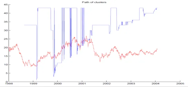
This measure is useful to see the transitions between the states. Comparing it with the graphics of the markets mean value it is possible to understand each state or transition that is happening during a certain period. This projection turns out to be very useful in understanding the clustering result, because the clustering result is compared with the time series.
Figure 13 - Path between Clusters example
36
3.5.3 Centroids distances measures
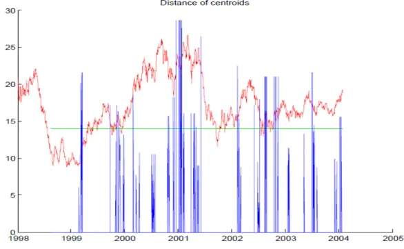
The centroids distance measures is used to measure the distance between the clusters, represented in cluster 13. This index is useful to compare transitions between far clusters with time series events.
This measure can also be seen as an instability measure. When compared with the time series we can see when there are big distances between clusters centroids where there is a big difference in the value variance between the two clusters. In the figure below there is a representation of this measure with the blue colour. The green line represents the mean value of the distances. The pe-riods that don’t have representation associated, it mean that the cluster hasn’t changed, so there is no distance associated with a cluster change.
37
Generator
3.6
The generator used for this study works based on a clustering result. The idea is to do a simulation with the states obtained by the SOM instead of using a total random generation like the Monte Carlo approach.
Based on the calculus of the current day variance to the previous day, each day will be grouped by the respective cluster and then the mean values and the standard deviation values (that is calculated based on the variance) from the cluster that were calculated.
With the previous result it is possible to make a simulation with the clus-ters information. Knowing the state order and state change, we only need to use the mean and standard deviation by state and generate a new value. To gener-ate the new value, the next calculus was used:
𝑑𝑎𝑦𝑉𝑎𝑟𝑖𝑒𝑛𝑐𝑒 = 𝑛𝑜𝑟𝑚𝑟𝑛𝑑(𝑚,̅̅̅ 𝜎)
, where the normrnd is a matlab function to generate a random value based in a normal distribution with the mean (𝑚̅) and the standard deviation (𝜎 ) from the respective cluster. After doing this we can calculate:
𝑑𝑎𝑦𝑉𝑎𝑙𝑢𝑒 = 𝑑𝑎𝑦𝐵𝑒𝑓𝑜𝑟𝑒𝑉𝑎𝑙𝑢𝑒∗ 𝑑𝑎𝑦𝑉𝑎𝑟𝑖𝑎𝑛𝑐𝑒
,where the 𝑑𝑎𝑦𝐵𝑒𝑓𝑜𝑟𝑒𝑉𝑎𝑙𝑢𝑒 represents the stock simulated value of the day before and the result will be the current day stock simulated value. It has to be considered that the first iteration didn’t have a 𝑑𝑎𝑦𝐵𝑒𝑓𝑜𝑟𝑒𝑉𝑎𝑙𝑢𝑒 so the real value
4
Clustering Technique Validation
This part of the thesis was important to validate the clustering algorithm being used. The objectives of these tests were to measure the precision of the cluster-ing algorithm by clustercluster-ing with some well-known problems of clustercluster-ing.
Two well-known data sets for this purpose were used: the wine dataset [47] and the iris dataset [48]. It also was used a synthetic dataset based on gen-erated values to validate the clusters results with a time series data. This valida-tion gave promising results, and also confidence to use the algorithm in the next section, that was testing with the financial data.
To measure the clustering quality it was chosen the Calinski-Harabasz index. The presented results were the ones that maximize the result of the in-dex. This estimation will decide the number of clusters that the algorithm will produce for the study.
40
Wine Data Set
4.1
The next image shows the clustering algorithm processes with the wine dataset. The first transition represents the formation of the Local Mins, and the second transition represents the clusters formation by the flooding technique. It can be seen four large blue zones that represent the four more important (populated) clusters.
Figure 15 - Flooding Evolution Wine
41
Figure 16 - CH Graphic Wine
To analyse the precision of the method, a confusion matrix, represented in the next table, was used. With this analyse it is possible to see the predicted class entities and the actual class entity. We can see that the predicted class pre-sents a reduced number of wrong predicted entities. By a simple calculus of sum of the wrong predicted entities and dividing it by the total number of enti-ties, we have a percentage of error of 2.8 %.
Confusion Matrix: 0,9 Deep
Predicted Class
Class 1 Class 2 Class 3
Actual Class
Class 1 57 2 0
Class 2 0 67 3
Class 3 0 0 47
Table 1- Confusion Matrix Wine
It can be concluded that the clustering algorithm tested with the Wine Da-taset resulted in a very good solution. The 5 units that had a wrong prediction were already bad classified by the SOM algorithm because within some BMUs that the SOM presented, entities of different classes were found. This resulted in error propagation for the clustering algorithm.
0 20 40 60 80 100 120
0,1 0,2 0,3 0,4 0,5 0,6 0,7 0,8 0,9 1 1,1 1,2 Deep Value
Calinski Harabasz Index
42
Iris Dataset
4.2
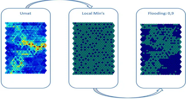
In the next figure it is possible to see the evolution of the clustering algorithm in the Iris Dataset. We can see U-matrix, the local min’s and finishing with the flooding algorithm result. It is possible to see the evolution from the Umat to the local min’s where the zones with closer neurons form more local min’s. On the transition from the local min’s to the result of flooding it is possible to see of the joining the zones with more density of local min’s.
Figure 17 - Flooding Evolution Iris
43
Figure 18 - CH Graphic Iris
The next table presents the true positives and false positives of the Iris taset. The error percentage was 26.7%. This results compared with the Wine Da-taset is less precise. It just reflects the difficulty of clustering the Iris DaDa-taset but also the need of a self-adapting clustering algorithm for clustering certain zones. With a less deep measure when clustering the Iris Versicolour or Iris Virginica classes, the separation of the two classes would be more expressed, reducing the error of the algorithm.
Confusion Matrix: 0,9 Deep
Actual Class
Iris Setosa Iris Versicolour Iris Virginica
Actual Class
Iris Setosa 50 0 0
Iris Versicolour 0 50 0
Iris Virginica 0 40 10
Table 2 - Confusion Matrix Iris
0 100 200 300 400 500 600
0,1 0,2 0,3 0,4 0,5 0,6 0,7 0,8 0,9 1 1,1 1,2 1,3 1,4 1,5 1,6 1,7 1,8 1,9 2 2,1 2,2 2,3 2,4 2,5 2,6
Deep Measure
Calinski Harabasz Index
44
Synthetic Time Series
4.3
It was generated a synthetic dataset to test the proposed approach when using the cluster technique in a time series dataset. The construction of the dataset used 4 different normal distributions, which generate 4 different trends in a time series. Based on this, 11 data series were generated that would serve as an input to the clustering algorithm.
The 4 different normal distributions had the flooding parameters:
𝑓(𝑥) = 𝑛𝑜𝑟𝑚(𝑚̅ , 𝜎) {
𝑚̅ = 1.4 𝜎 = 20 𝑖𝑓(1 ≤ 𝑥 ≤ 500) 𝑚̅ = −1.4 𝜎 = 20 𝑖𝑓(501 ≤ 𝑥 ≤ 1000)
𝑚̅ = 1.4 𝜎 = 20 𝑖𝑓(1001 ≤ 𝑥 ≤ 1500) 𝑚̅ = −1.3 𝜎 = 20 𝑖𝑓(1501 ≤ 𝑥 ≤ 2000)
, where 𝑚̅ assumes the mean value and 𝜎 assumes the standard deviation parameter. By analysing the function we will have a positive variation during two sliding windows that will be the first 500 values and between the 1000 and 1500 values. The other two sliding windows generate numbers with negative variation.
The resulting time series dataset is presented in the next figure. As it can be seen it is impossible to detect any pattern by human observation.
45
The result of clustering with the SOM algorithm is presented in the Figure 20. To generate this image, the mean of the previous time series was used, rep-resenting the single time series in the figure. By this it is better understood the trends of the time series and it is possible to project the clusters in the time se-ries. The clustering result is represented over the time series, where different colors represent different clusters.
Figure 20 - Cluster over synthetic time series
The clustering showed uses a deep measure of 1.3, and is presented with 7 clusters. Four of the 7 clusters have less than 12 entities, so they weren’t repre-sented in this graphic.
46
Figure 21 - CH Synthetic Time Series 0
500 1000 1500 2000 2500 3000
0,1 0,2 0,3 0,4 0,5 0,6 0,7 0,8 0,9 1 1,1 1,2 1,3 1,4 Deep Measure
Calinski Harabasz Index
5
Application to Financial Data
This chapter will present the results of clustering with financial data. The data used in this paper is based on the sp500 index companies. The companies of this index correspond to the 500 biggest companies in US, making the usual in-vestors picks for analyses and trading. The period being studied starts at 2004 and ends in 2014. In this period it is possible to see the impact of the most recent crisis which started in 2007 and started recovering at 2009.
For this datasets it will be processed a selection of two sets with correlated and inverse-correlated stock values. This will allow seeing the impact of the states produced during the pre-crises, crises and pos-crises. It was also analysed studies of states importance and analyses of distances transitions.
To finish it will be analysed the result of generating a price time series based on the previous analyses of the clustering algorithm.
48
Correlation Method
5.1
The correlation method is a calculus to measure the relation of two time series. For this purpose it was used a simple form that looks at the two time series trends to see if they are similar to each other.
The calculus measures the correlation based in a time interval. The higher the value the more correlated the time series were, using the sum of the scores available. The 𝑚𝑖𝑛 𝑇 represents the minimal length for both time series and the time is the length of the time interval that will be measured in the score func-tion. So by definition as much as it is scored the better the correlation is.
Based in:
score(x, y) = {1, 0, trend(x) = trend(y)trend(x) ≠ trend(y) (24)
We have:
𝜑 = ∑ 𝑠𝑐𝑜𝑟𝑒(𝑥𝑡, 𝑦𝑡) min 𝑇
𝑡=𝑡𝑖𝑚𝑒
(25)
This method was designed to look for similar trends behaviour and not to the variance of the data set. The impact of big and small variations in the time series will be analysed by the SOM algorithm, and based in that, track particu-lar states.
Case Study One
5.2
49
Figure 22 - Correlated Companies
In the previous image it is possible to see that the trends of each stock are very similar with each other. Each company represents or is connected (only two are just connected) with the financial sector of real estate investment indus-try. This shows how the companies of real estate represent the same behaviour and where affected by the same factors.
This companies still survived to the crises of 2007 but it is evident the huge crises effect over these group. With this result it was interesting to see the states produced before and after the crises, and see if there is a presence of a state that may be associated with a pre-crises or pos-crises pattern.
So with this dataset we proceeded to the SOM classification with the flooding parameter adjusted to the max Calinski-Harabasz index. After that, it was possible to analyse the results with the state study measures (the three ap-proaches presented in the 3.5 section).
50
Var1: Simon Property Group
Var2: Macerich,
Var3: Boston Properties
Var4: Public Storage
Var5: Simon Property Group Inc.
Var6: AvalonBay Communities Inc.
Var7: Prologis,
Var8: Equity Residen-tial
Var9: Apartment In-vestment & Mgmt
Var10: Ventas Inc.
Var11: HCP Inc.
Figure 23 - UMAT and Component Planes Correlated Markets
In the image bellow it is possible to see the impact that certain cluster had in the time series. Cluster number 33 has more entities than all the other clusters together. In the representation of the time series it is possible to see that the cluster 33 appears during a long period and this period corresponds to positive variance of the stock market value.
Figure 24 - Clusters Size (left side) and Clusters Transitions (right side)
51
time series. In the distance graphic in the next figure it is possible to see a great variance of the stock value between crises states. The clusters in crises periods change more often and to longer distances comparing to long periods of no change or of small distant clusters. Between the year of 2008 and 2009 (crises period) the distance measure assumes very unusual values, showing the insta-bility of the states.
Figure 25 - Distance Clusters (Left Side) and Colour Clusters (right side)
In the colour clusters graphic in Figure 25 - Distance Clusters (Left Side) and Colour Clusters (right side) it is possible to see the representation of the clusters that have more entities directly in the time series. In the figure is repre-sented the cluster 33 (green coloured), the cluster 39 (red coloured), the cluster 34 (blue coloured) and the rest of the clusters black coloured. It is possible to see that a great part of the time series is represented by the cluster 33 that repre-sents most of the period where the time series had a positive variation.
Analysing the crisis period in the colour clusters graphic its notable the importance of the cluster 39 and cluster 34. During this period these clusters were active by a longer and repeated period comparing with the rest of the time series.
52
Figure 26 - Correlated Markets Simulation
In the previous image it is possible to see how close the two time series are and also how equal both presented trends are. Another interesting factor is the behaviour of the simulated time series during the crisis period (it is represented between the two blue dotted lines), where it is possible to see a high value of instability comparing to the period before crises.
In the next image it’s shown an experiment that was generating 15 time series. Analysing the result it can be seen an instability behaviour during the crisis period (between the 750 and 1400). On other hand the time series experi-ments a stable behaviour when it is not in the crisis state.
53
Inverse-Correlation Method
5.3
The Inverse-Correlated method uses the same principle of the correlated meth-od but the score function changes. So for this methmeth-od we have:
score(x, y) = {0, 1, trend(x) = trend(y)trend(x) ≠ trend(y) (26)
So the score function sets the value to 1 when two trends have a different behaviour. With this it will be possible to track series that are inverse-correlated with a specific sock value series.
This type of analyses is also important because of its potentiality to project a prediction of a crisis state. It will be possible to detect through the analyses of behaviour of inverse-correlated markets before reaching a crisis state.
Case Study Two
5.4
Based on the correlated method it was selected the most inverse-correlated company from the sp500 index. The company selected was Dell Inc. that represents the Information Technology sector from the Computer Hard-ware industry. The top 10 correlated companies were Mylan Inc., Brown-Forman Corporation, Lilly (Eli) & Co., United Health Group Inc., Jabil Circuit, People's United Bank, Gilead Sciences, SCANA Corp, The Hershey Company, Nucor Corp. Most of the companies were from the health care sector.
In the figure it is showed the referenced companies.
Figure 28 - Inverse-Correlated Time Series
54
doesn’t seem to have any type of similarity with the other stocks. With a closer analyse it is possible to see, during the 2007 crisis, most of the stock’s values went in a negative trend.
With this data set, the SOM algorithm and the cluster algorithm were exe-cuted. The result of the SOM with the component planes is shown in the next image. It is possible to analyse how different the component planes are from each other. Also, by analysing the U-matrix it is possible to see how the clusters are well defined.
Var1: Dell Inc Var2: Mylan Inc. Var3: Brown-Forman Cor-poration
Var4: Lilly (Eli) & Co. Var5: United Health Group Inc.
Var6: Jabil Circuit Var7: People's United Bank Var8: Gilead Sciences Var9: SCANA Corp Var10: The Hershey Com-pany
Var11: Nucor Corp
Figure 29 - UMAT and Component Planes Correlated Markets
55
Figure 30 - Clusters Size (left side) and Clusters Transitions (right side)
In these results it’s quite notable that there are more clusters but less data by cluster. In the previous image it is possible to see that there are some clusters with almost 100 entities of data, but there are many with less data. In this test Calinski-Harabasz didn’t give the intended deep value and pointed to a low deep measure. The right graphic from Figure 31 shows that the clusters aren’t really stable and that the data is always changing from cluster to cluster.
Figure 31 - Distance Clusters (Left Side) and Colour Clusters (right side)
56
As in the previous study, it was generated a price time series based on the clustering obtained by the SOM algorithm. The result is represented in the next image.
Figure 32 – Inverse-Correlated Markets Simulation
The 2007 crisis is represented between the blue dotted lines. The same pat-tern of instability that was seen in the previous result can be seen again. Time period before crisis is very stable and seem to increase with less variance com-pared with the period when the time series is decreasing.
57
![Figure 1 - Local correlation scores [7]](https://thumb-eu.123doks.com/thumbv2/123dok_br/16526863.736018/21.892.336.648.245.605/figure-local-correlation-scores.webp)
![Figure 3 - Hurst Index [12]](https://thumb-eu.123doks.com/thumbv2/123dok_br/16526863.736018/25.892.269.660.134.455/figure-hurst-index.webp)
![Figure 6 - Self-organizing map structure, referenced from [21]](https://thumb-eu.123doks.com/thumbv2/123dok_br/16526863.736018/30.892.326.566.136.433/figure-self-organizing-map-structure-referenced.webp)