GBT MODEL FOR THE BUCKLING ANALYSIS OF CONICAL SHELLS WITH STRESS CONCENTRATIONS

Lisbon, Portugal, July 24-27, 2018

GBT MODEL FOR THE BUCKLING ANALYSIS OF CONICAL

SHELLS WITH STRESS CONCENTRATIONS

Adina-Ana Mureșan*, Rodrigo Gonçalves** and Mihai Nedelcu*

* Technical University of Cluj-Napoca, Faculty of Civil Engineering, Romania e-mails: [email protected], [email protected]

** CERIS, ICIST and Faculty of Sciences and Technology, Universidade Nova de Lisboa, Portugal e-mail: [email protected]

Keywords: Generalized Beam Theory; Conical shells; Finite element method; Linear buckling analysis.

Abstract. The paper presents a Finite Element formulation based on Generalized Beam Theory (GBT) for the analysis of the linear buckling behaviour of conical shells under various loading and boundary conditions. The GBT approach provides a general solution for the 1st and 2nd order analyses using bar elements capable of describing the global and local deformations. Because of the cross-section variation specific to conical shells, the mechanical and geometric properties are no longer constant along the bar axis as in the case of cylinders and prismatic thin-walled members. This proposed GBT finite element formulation is validated by comparison with results obtained by means of shell finite element analyses. The illustrative examples cover axially compressed members displaying all classical bar boundary conditions. Special attention is dedicated to the effect of pre-buckling stress concentrations.

1 INTRODUCTION

The stability of cylindrical and conical structures has been studied from the analytical and experimental point of view since the beginning of the 20th century. At first the small deflection theory was used for obtaining bifurcation buckling solutions of shell structures [1], [2]. However, experimental results showed that cylinders buckled at loads well below those predicted by the small deflection theory. Donnell proposed a non-linear theory for circular cylindrical shells under the simplifying shallow-shell hypothesis [3]. Depending on the non-linear strain components considered, other large deflections theories were subsequently proposed by Sanders [4], Flügge [5] and Novozhilov [6].

Von Karman and Tsien performed a seminal study on the stability of axially loaded

circular cylindrical shells, based on Donnell’s nonlinear shell theory [8]. Later, Donnell and Wan showed that the imperfections are the cause of the large differences between the analytical and experimental results of the stability analysis of cylindrical structures [9]. Weingarten et al. studied the elastic stability of thin-walled cylindrical and conical shells under axial compression in an experimental manner and showed that the buckling coefficient varies with the radius-to-thickness ratio [10]. Mushtari and Sachenkov determined an upper limit of critical bifurcation loads of cylindrical and conical structures with circular cross section subjected simultaneously to axial compression and external normal pressure [11]. Tovstik studied the stability of thin elastic cylindrical and conical shells by assuming that buckling is accompanied by the formation of a large number of dents which depend on the

initial stresses and on the curvature of the shell’s middle surface [12].

first studies which extend GBT to the 1st order analysis and the buckling analysis of cylindrical shells were developed by Christof Schardt and Richard Schardt [13], [14] and [15]. Silvestre developed further this field by studying the buckling (bifurcation) behaviour of circular cylindrical shells subjected to axial compression, bending, compression plus bending and also torsion [16]. Also, Silvestre developed a GBT formulation capable of assessing the buckling behaviour of elliptical cylindrical shells subjected to compression [17].

Nedelcu developed a GBT formulation for the buckling analysis of isotropic conical shells [18]. The paper studies conical shells subjected to axial compression having different boundary conditions. As in the GBT formulation for thin walled prismatic bars with variable cross section developed by the same author [19], the mechanical and geometrical properties

are no longer constant along the member’s length. However, in the case of conical shells,

these properties can be easily defined. Moreover, the buckling modes turned out to be a combination of shell-type deformation modes which can be easily pre-determined. The validation of the GBT formulation for conical shells was done by comparing the results obtained by the GBT analysis of conical shells having different boundary conditions with the results obtained by Shell Finite Element Analysis (SFEA). In [18], the GBT system of equilibrium equations was solved using the Runge-Kutta Lobatto IIIA collocation method of 4th order [20]. The method proved to have limitations in case of structures subjected to arbitrary loading and boundary conditions. Also, the method proved to be unstable in case of a large number of coupled deformation modes. For these reasons, a GBT-based Finite Element (FE) formulation seems preferable. Such type of FE is already used by many researchers to analyse the buckling behaviour of prismatic thin-walled members and structures under arbitrary loading and boundary conditions [21], [22].

The following paper presents a GBT-based Finite Element (FE) formulation to analyse the elastic bifurcation behaviour (according to the linear bifurcation analysis concept) of isotropic conical shells with stress concentrations using the Love – Timoshenko large deflection shell theory [7]. The analyzed members are subjected to axial compression and the effect of the pre-buckling stress concentrations is assessed. The analysis is divided into two steps: (i) a 1st order analysis from which the pre-buckling stresses are computed exactly, including boundary effects, and (ii) a linear bifurcation analysis using the meridional and circumferential stresses obtained from the 1st order analysis.

The GBT-based FE analysis is implemented in Matlab [23]. For the validation of the results, several models were created in Abaqus [24] using shell finite elements. The methodology was validated by comparing the results obtained using the proposed formulation and SFEA.

2 GENERALIZED BEAM THEORY FOR CONICAL SHELLS

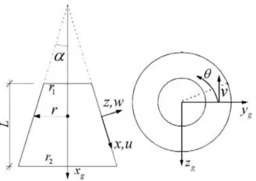
The GBT adaption for conical structures was presented in detail in [18], therefore this section briefly describes the main aspects. Figure 1 presents the geometry of a conical member (length L, thickness t, semi-vertex angle α), the global coordinate system xg, yg and zg

and the local coordinate system x, θ and z, where: x∈[0, L cos α⁄ ] is the meridional coordinate,

Figure 1: The geometry of conical shell.

The strains can be decomposed according to:

 

     

 

where: {εM}, {εB} are the membrane and bending strains, respectively, and {χ} is the vector of variation of curvature with respect to the reference surface.

According to Love – Timoshenko theory [7] the kinematic relationships have the following expressions in case of conical shells [25] having linear and non-linear components:

             2 2 2 , 2 , , .

. x x

x NL M xx L M xx M xx v w u                                       2 , 2 , , . . 2 1 2 1 r wc v r w vc r us r wc r v NL M L M

M   

                          r v v r c vw r w w r vs v r

u _{x x x}

x NL M x L M x M x          , , , , , , , . . (2) xx xx w,  2 , , 2 , r c v r s w r

w_{ x }                       r vs v r c r s w r

w _{x x}

x

2 2 , ,₂ ,





with the notation s=sinα and c=cosα.







k x v v x w w x

u u 1 1 1 ) , ( , ) , ( , ) ,

(    (3)

where n is the number of cross-section deformation modes.

The GBT product formulation is next used to describe each component:

 

 

k _{k k x}

k _{k k k k}

k

k _{k k k}

u x u r x x

v x v x u x

u

w x w x x

c                      (4)

where uk(θ), vk(θ), wk(θ) are the cross-section displacement functions pertaining to mode k and ϕk(x)is the corresponding modal amplitude function defined along the member’s length. The

above expressions were chosen in order obtain null membrane shear strains γ_xθM.L and transverse strains ε_θθM.L (the components –vs/r and us/r are neglected).

Let us consider the first variation of the strain energy according to the linear stability analysis concept,







xx dzrd dx

W       0 0  0   0

 _{       } (5)

whereσ_xx0 , σ_θθ0 and τ_xθ0 are the pre-buckling meridional, circumferential and shear stresses, respectively, due to the applied external loads.

The constitutive relations are the following:

             x x xx xx xx Q Q Q Q Q 33 22 21 12 11      (6)

where Q11=Q22=E/(1-μ2), Q12=Q21=μQ11 and Q33=G. E and Gare Young’s and shear moduli

and μis Poisson’s ratio.

Using the kinematic relations from equation (2), the constitutive relations from equation (6) and operating all the integrations over the circumference and thickness, the strain energy is expressed as follows:





X X X G G B D D D C W

L kx ix jik k i jik k ix kx i x jik i x k ki x i k ik i k ik i xx k ki xx i k ik xx i k ik xx i xx k ik



where: Cik, Dik1, Dik2, Bik, Gik are mechanical stiffness matrices related to general warping,

2.1 Shell-type deformation modes

In order to diagonalize the mechanical stiffness matrices as much as possible, one aims to determine the warping functions uk(θ) that simultaneously fulfil all the orthogonality

conditions:







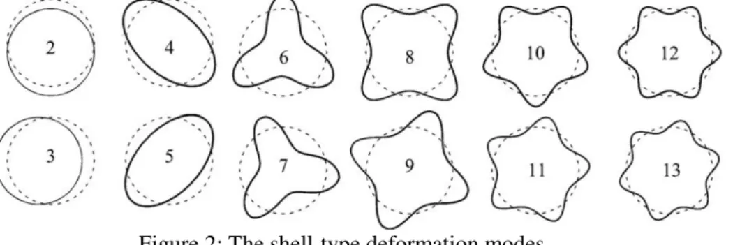
In case of circular cross sections there are two independent sets of trigonometric functions extensively used in other studies [7], [16] which fulfil the orthogonality conditions:

  

   

, 2 ) 1 ( ),

cos(

, 2 ),

sin(

k m m

k m m

u_k

 

1 ,..., 5 , 3 , 1

,..., 6 , 4 , 2

 



n k

n k

(9)

For a given m there are two similar modes with distinct order k. This is the reason why in the buckling analysis of uniformly compressed members there is always a set of two buckling modes with equal critical loads.

The independent trigonometric functions from equation (9) define the shell-type deformation modes, whose in-plane configurations are shown in Figure 2.

Figure 2: The shell-type deformation modes.

Introducing the warping functions previously described into the expressions of the mechanical stiffness and geometric matrices, leads to simplified formulas depending only on the material coefficients, semi-vertex angle, current radius and deformation mode number. These formulas were also given in detail in [18].

As r varies along the length, the elements of the stiffness matrices are not constant along the longitudinal axis. Thus, in the expression of the variation of strain energy, the elements of the stiffness matrices are also integrated along the member length.

2.2 Additional deformation modes

 

   

 

   

 

   

k _{k k x}

k _{k k}

k _{k k}

u x u x

v x v x

w x w x

            (10)

For each additional deformation mode, the cross-section displacements are described as follows:

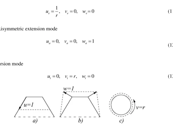
2.2.1 Axial extension mode

0 ,

0 ,

1 _{ }

 _{e e}

e v w

r

u (11)

2.2.2 Axisymmetric extension mode

1 ,

0 ,

0  

 a a

a v w

u

(12)

2.2.3 Torsion mode

0 ,

,

0  

 t t

t v r w

u (13)

Figure 3: The additional deformation modes: a) axial extension, b) axisymmetric extension, c) torsion.

For the axially compressed members studied in this paper, the deformation resulting from a 1st order analysis is characterised by a coupling of the first two additional modes: the axial extension mode (e) and the axisymmetric extension mode (a). Since there is no shear, the variation of the strain energy for the 1st order analysis reads:







xx dzrd dx

W     

 _{, , , ,} (14)

where i, k can be any of the modes e or a.

Introducing equation (11) and equation (12) together with the kinematic and constitutive relations given by equation (2) and equation (6), the variation of the strain energy becomes:



L ki kxx ix ik kx i

xx i x k ik i k ik i xx k ki xx i k ik x i x k ik xx i xx k ik dx F H H B D D D C W                  , , , , , , 2 , 2 , , 1 , , (15)

2.2.4 For the axial extension mode 0 , 2 , 0 0 , 2 , 2 2 2 2 1 1 1       ee ee ee ee ee ee F s A H B D r s A D r A C    (16)

2.2.5 For the axisymmetric extension mode

0 , 2 , 2 0 , 2 , 2 2 2 1 2 2 1 1 1       aa aa aa aa aa aa F s D H r c A B D r s A D r D C     (17)

2.2.6 For the coupling of extension-axisymmetric modes

r sc A F H B c A D D C ea ea ea ea ea ea 1 2 2 1 2 , 0 , 0 2 , 0 , 0         (18)

where: A1=Et/(1-μ2), A2=μA1, D1=Et/(12(1-μ2)), D2=μD1.

3 THE FINITE ELEMENT FORMULATION

The GBT eigenvalue problem for linear buckling (bifurcation) can be solved by analytical methods (for very simple cases) or by approximate methods (e.g. FEM). In the case of conical shells, initially, a Runge-Kutta numerical method was used in [18] namely the Lobatto IIIA 4th order collocation method [20]. The method proved to have limitations in case of structures subjected to arbitrary loading and boundary conditions. Also, the method proved to be unstable in case of a large number of coupled deformation modes. In this paper a FE formulation previously used for prismatic members ([21], [22]) was adapted for the special case of variable cross-section along the member axis and it is based on the variation form of the strain energy given by equations (5) (bifurcation analysis) and (14) (1st order analysis).

The shape functions to approximate the modal amplitude function ϕk(θ)(see equation (4))

are the classic cubic Hermitian polynomials expressed as follows:









4 2 3 3 2 3 2 2 3 1 3 2 , 1 3 2 , 2                         e e L L (19)

where Le is the length of the finite element and ξ=x/ Le.

Therefore, the modal amplitude function ϕk(θ) is approximated in the following form:

 

_k x d d d d (20)

where: d1=ϕk,x(0), d2=ϕk(0), d3=ϕk,x(Le) and d4=ϕk(Le) are the degrees of freedom (DOF) of

the FE, leading to 4n DOF per mode (2n DOF per node).

 

 

 





 

_{ }

0

  e e e

d G

K  (21)

where: [K(e)], [G(e)] are the finite element linear stiffness matrix and geometric stiffness matrix, respectively and {d(e)} is the displacement vector.

The components of matrices [K(e)] and [G(e)] are obtained from the following expressions:



L ik p rx ki px r

r p ik r xx p ki xx r p ik x r x p ik xx r xx p ik ik pr dx G G B D D D C K               , , , 2 , 2 , , 1 , , (22)







pr X X dx

G  _, _,   (23)

where: i,j=2…n and p,r=1…4 (p,r are the indexes of the DOF).

For the first order analysis, only the linear stiffness matrix is retained, which for axial compression has the following expression:

1 2 2

, , , , , ,

, , , , ,

e

ik p xx r xx ik p x r x ik p r xx ki p xx r ik p r ik

pr

L ik p x r xx ki p xx r x ik p x r

C D D D B

K dx

H H F

                       _ _     



where i, k can be any of the axial extension or axisymmetric extension deformation modes.

The arbitrary external forces are replaced by equivalent “nodal” forces acting as distributed

loads at the end cross-sections of the finite element. The FE force vector f(e) is obtained from:

0 _

0 _ 0 _ _ _ _ 0 0 0 0 0 0 x i y z i i Le x i Le y Le z

f

u

f f

f v rd

f w f f            _{ }   _{  }     _{  } _{ }   



where f0and fLe are the equivalent distributed loads acting at the FE end cross-sections and the

second index (x, y or z) is specifying the projection on the corresponding local axis. For the axially compressed finite element loaded with an axial force P0 at the starting node (x = 0),

the force vector reduces to:





( )

0cos 0 0 0 0 0sin 0 0

T e

f  P  P  (26)

where the first 4 components are related with the axial extension mode and the other 4 components are related with the axisymmetric extension mode.

The principle of virtual work leads to the standard linear equation:  e

 

 

K d f

  

  (27)

Because conical shells have variable cross section, the mechanical and the geometric

illustrative examples, the authors used 4 integration points, due to the fact that more points did not improve the solution.

The GBT-based finite element formulation starts by dividing the member into the desired number of finite elements. The nodal degrees of freedom are identified and they are grouped in vector {d}. The finite element stiffness matrices are assembled to form the global linear stiffness matrix [K] and the global geometric stiffness matrix [G]. The same applies for the external force {f} and displacement {d} vectors. For the 1st order analysis solving the linear equation system [K]·{d}={f} leads to the displacement vector {d} from which the pre-buckling strain and stress fields are computed. Next the bifurcation analysis is performed using the pre-buckling stresses and the solution of the eigenvalue problem [K+λG]·{d}={0} leads to the eigenvalues λ, with the lowest value being the critical value λcr, and the corresponding

buckling modes represented by the eigenvectors {d}.

In order to determine a deformed configuration of the thin-walled member, the modal amplitude function ϕk(x) is determined from the superposition of the shape functions ψi(ξ)

using (20) and next, the displacement field is found using equation (4) and equation (3).

4 NUMERICAL EXAMPLES

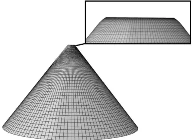
In order to validate the proposed formulation for the analysis of conical shells under axial compression, several numerical examples were considered. Let us consider the conical shell from Figure 4. The conical shell is made of steel (E=210GPa, μ=0.3), the thickness of the wall is t=1 mm and the length is L=1200 mm. The top radius is r1=50 mm, while the bottom

radius r2 is variable, having values ranging from 50 to 1000 mm.

The members with stress concentrations have the top end free to all displacements/rotations, a region where the loading is introduced, leading to significant local end effects. These end effects are given by local deformations (see Figure 5) and local large variations of the pre-buckling circumferential normal stresses provided by the 1st order analysis, in the free end region (see Figure 6 and Figure 7 – the free end is located at the left-hand side). In these figures the bottom radius was considered to be r2 = 1000 mm. These

concentrations of the pre-buckling stresses can no longer be neglected nor approximated by simple formulas (see Eq. 28).

Figure 4: The geometry of the analyzed conical shell.

The loading is introduced as P=λ·P0, where λ is the loading coefficient, P0 is the value of

the axial force used in the 1st order analysis and, for all cases, P0=1 kN. The proposed

The SFEA were carried out in Abaqus [24] with S4 rectangular shell finite elements. The size of the mesh varies along the length having a dimension around 5 mm at the top end and 50 mm at the bottom end.

For the special case of axial compression, the 1st order deformation is characterized by a coupling between the axial extension and the axisymmetric extension deformation modes. The buckling modes are characterized by a single shell-type deformation mode. It should be stressed that having no deformation mode coupling leads to great computational economy, an advantage impossible to achieve with shell finite elements. In particular, all the GBT matrices are nxn diagonal matrices and the FE matrices K(e) and G(e) are 4nx4n matrices, essentially banded, formed by diagonal addition of 4x4 matrices (there are 4 DOF per deformation mode).

Figure 5: The free end displacements of an axially compressed cantilever conical shell resulting from SFEA. The displacement scale factor is 200.

Figure 6: The pre-buckling meridional stresses σ_xx0 of an axially compressed cantilever conical shell with r2=1000mm.

-4 -3,5 -3 -2,5 -2 -1,5 -1 -0,5 0

0 200 400 600 800 1000 1200

Me

rid

io

n

al

str

ess

es

[N/m

m

2

]

Figure 7:The pre-buckling circumferential stresses σ_θθ0 of an axially compressed cantilever conical shell with r2=1000mm.

The meridional and circumferential normal stresses σ_xx0 and σ_θθ0 determined in the 1st order analysis were subsequently used in the buckling analysis, to determine the geometric tensors

Xjikσθ and Xjikσx (equation (7) which take into consideration the second-order effects and they are

used to to determine the elements of the FE geometric stiffness matrix (equation (23)).

4.1 Cantilever conical shells

The analysed members have the top end free to all displacements/rotations, while the bottom end is fixed. Figure 8 presents the critical buckling modes and the corresponding buckling coefficients λc for conical shells having different values of the radius r2. The figure

also illustrates the buckling coefficients obtained with SFEA and the relevant cross-section deformation modes k. In the conical shells’ buckling modes one can observe the end effects

that occur at the cantilever’s free end.

Figure 8: The buckling modes of cantilever conical shells resulting from SFEA.

To demonstrate the importance of taking into account the 1st order local end effects, a simplified analysis was carried out, in which the pre-buckling stresses σ_θθ0 were neglected, and the pre-buckling stresses σ_xx0 were approximated by the following equation:

rtc P xx _



2

0 _

(28) -40

-35 -30 -25 -20 -15 -10 -5 0 5 10

0 200 400 600 800 1000 1200

C

ir

cu

m

fer

en

tial

str

ess

es

[N/m

m

2

]

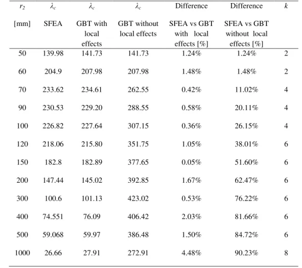
Table 1 shows the comparison between the rigorous and the simplified approach. The results were compared with respect the critical buckling coefficient obtained from SFEA. The simplified approach provided errors reaching up to 91% for large values of r2, proving the fact

that the local end effects must be taken into account for the analysis of conical shells with free-loaded ends.

The large variations of the pre-buckling stresses are produced on a small region near the free end where the FE mesh should be refined enough to capture them. To test the precision and stability of the proposed formulation, two case studies were considered for the analysed numerical examples: (i) finite elements having constant length and (ii) finite elements having variable length. In Abaqus the size of the SFE-s varies linearly between approximatively 5 mm at the free end and 50 mm at the fixed end.

Table 1: SFEA results vs. GBT results when local end effects are taken/not taken into account.

r2

[mm]

λc

SFEA

λc

GBT with local effects

λc

GBT without local effects

Difference SFEA vs GBT

with local effects [%]

Difference SFEA vs GBT

without local effects [%]

k

50 139.98 141.73 141.73 1.24% 1.24% 2

60 204.9 207.98 207.98 1.48% 1.48% 2

70 233.62 234.61 262.55 0.42% 11.02% 4

90 230.53 229.20 288.55 0.58% 20.11% 4

100 226.82 227.64 307.15 0.36% 26.15% 4

120 218.06 215.80 351.75 1.05% 38.01% 6

150 182.8 182.89 377.65 0.05% 51.60% 6

200 147.44 145.02 392.85 1.67% 62.47% 6

300 100.6 101.13 423.02 0.53% 76.22% 6

400 74.551 76.09 406.42 2.03% 81.66% 6

500 59.068 59.97 386.48 1.50% 84.72% 6

1000 26.66 27.91 272.91 4.48% 90.23% 8

4.1.1 Finite elements with constant length

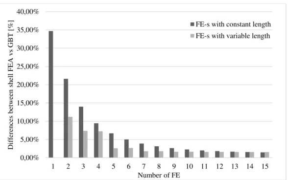
In the following case study, the conical shells modelled using the proposed formulation are meshed with finite elements having constant length. Figure 9 presents the differences between the results obtained using SFEA and the results obtained using the GBT based FE formulation for a cantilever conical shell with r2=500 mm. In the GBT based FE formulation model the

4.1.2 Finite elements with variable length

In this case study, the conical shell of the preceding example (r2=500 mm) is analyzed

using the proposed formulation, meshed with finite elements having variable length. At the

conical shell’s free end (in the “local effects” region) on a meridional length equal with r1/cosα, where r1 is the top radius, the finite elements have equal length producing a refined

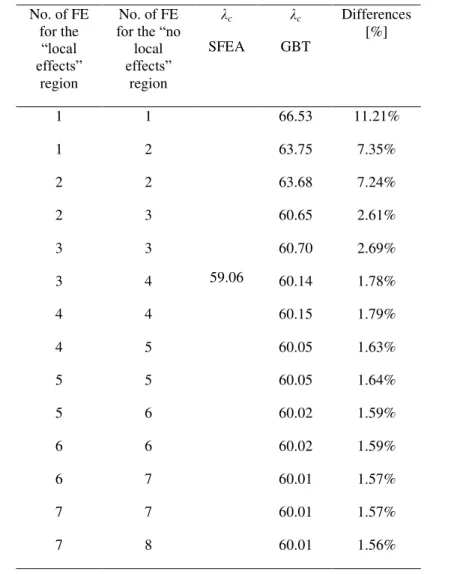
mesh. For the rest of the member, the length of the finite elements increases linearly producing a coarse mesh (in the “no local effects” region). Table 2 presents the results obtained for various discretization schemes and also the SFEA result. The results are compared in Figure 9 with the values obtained using FE-s with constant length. It can be observed that the differences between the SFEA and the GBT results are now below 3% for only 5 FE-s (2 for “the local effects” region and 3 for the “no local effects” region).

Figure 9: The differences between the results obtained with SFEA and GBT for different numbers of GBT-based finite elements.

0,00% 5,00% 10,00% 15,00% 20,00% 25,00% 30,00% 35,00% 40,00%

1 2 3 4 5 6 7 8 9 10 11 12 13 14 15

Dif

fer

en

ce

s

b

etw

ee

n

s

h

ell

FEA

v

s

GB

T

[

%]

Number of FE

Table 2: The differences between SFEA vs. GBT for different sizes of the FE mesh.

No. of FE for the

“local effects”

region

No. of FE

for the “no

local

effects”

region

λc

SFEA

λc

GBT

Differences [%]

1 1

59.06

66.53 11.21%

1 2 63.75 7.35%

2 2 63.68 7.24%

2 3 60.65 2.61%

3 3 60.70 2.69%

3 4 60.14 1.78%

4 4 60.15 1.79%

4 5 60.05 1.63%

5 5 60.05 1.64%

5 6 60.02 1.59%

6 6 60.02 1.59%

6 7 60.01 1.57%

7 7 60.01 1.57%

7 8 60.01 1.56%

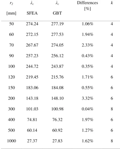
4.2 Cantilever conical shells with simple support in the middle of the span

In the following case study, a cantilever conical shell was considered which has an additional simple support in the middle of the span. As in the previous case, the conical shells have the free end corresponding to radius r1, and the fixed end corresponding to radius r2. In

the middle of the span, the cantilever has a simple support which allows warping and has the v and w displacements blocked. Figure 10 presents the buckling modes and Table 3 presents the differences between SFEA and GBT, as well as the relevant deformation mode number k. As in the previous case, the local end effects are present and they must be taken into account. By comparing the buckling coefficients given in Table 1 and Table 3 it can be concluded that the intermediate simple support makes the structure stiffer but only for small values of radius r2.

Figure 10: The buckling modes of the cantilever conical shells with simple support in the middle of the span resulting from SFEA.

Table 3: SFEA results vs. GBT results for cantilever conical shells with simple support in the middle of the span.

r2

[mm]

λc

SFEA

λc

GBT

Differences [%]

k

50 274.24 277.19 1.06% 4

60 272.15 277.53 1.94% 4

70 267.67 274.05 2.33% 4

90 257.23 256.12 0.43% 4

100 244.72 243.87 0.35% 4

120 219.45 215.76 1.71% 6

150 183.06 184.08 0.55% 6

200 143.18 148.10 3.32% 6

300 101.03 100.98 0.04% 8

400 74.81 76.32 1.97% 6

500 60.14 60.92 1.27% 6

1000 27.37 27.83 1.62% 8

5 CONCLUSIONS

structural members with variable cross-section [18], [19]. This paper presented a GBT-based FE formulation to analyse the buckling (bifurcation) behaviour of isotropic conical shells with stress concentrations. The advantages of using this formulation in comparison with the classic SFEA are the following: much fewer DOFs are necessary to obtain similarly accurate results and the solutions for axially compressed shells are obtained with a single shell-type deformation mode. Furthermore, in a coupled instability problem, the proposed formulation provides the degree of modal participation – an aspect which will be addressed in a future paper concerning the buckling analysis of conical shells subjected to other types of loads.

From the numerical examples presented in this paper, three remarks can be highlighted. The first remark is related to the validation of the GBT based FE formulation for the buckling analysis of isotropic conical shells. The critical buckling coefficients obtained with SFEA and the ones obtained with the proposed formulation are in excellent agreement. The second remark is related to the flexibility of the proposed formulation. As seen from the numerical examples illustrated in the paper, the proposed formulation can be applied to any type of classic bar boundary conditions. The last remark refers to the local large variations of the pre-buckling stresses. In this respect it was shown that in the GBT pre-buckling analysis of conical shells with stress concentrations is extremely important to take into account the 1st order local end effects in order to have good results.

The proposed GBT based FE formulation can be applied for the buckling analysis of conical shells subjected to loads other than axial compression (i.e. pure bending, torsion, or complex loading conditions). These case studies are currently under work and will be presented in future papers.

REFERENCES

[1] Lorenz R. Achsensymmetrische verzerrungen in dünnwandingen hohlzzylindern. Z Vereines Deutscher Ing 1908;52(43):1706–13

[2] Love AEH. A treatise on the mathematical theory of elasticity, fourth Ed. New York: Dover; 1944.

[3] L. H. Donnel, “A New Theory for the Buckling of Thin Cylinders Under Axial Compression and

Bending,” Trans. Am. Soc. Mech. Eng., vol. 12, no. 56, pp. 795–806, 1934. [4] Sanders JL. Nonlinear theories for thin shells. Q J Appl Math 1963; 21(1): 21–36. [5] W. Flügge, Stresses in Shells, second ed. Springer, Berlin, 1973.

[6] V.V. Novozhilov, Foundations of the Nonlinear Theory of Elasticity, Graylock Press, Rochester, NY, USA (now available from Dover, NY, USA), 1953.

[7] Timoshenko S, Gere JM. Theory of elastic stability. New York: McGraw-Hill Book Company; 1961.

[8] T. von Karman and H.-S. Tsien, “The Buckling of Thin Cylindrical Shells Under Axial

Compression,” J. Aeronaut. Sci., vol. 8, no. 8, pp. 303–312, Jun. 1941.

[9] L. H. Donnel and C. C. Wan, “Effect of imperfections on the buckling of thin cylinders and columns under axial compression,” J. Appl. Mech., vol. 1, no. 17, pp. 73–83, 1950.

[10]V. I. Weingarten, E. J. Morgan, and P. Seide, “Elastic stability of thin-walled cylindrical and

conical shells under axial compression,” Am. Inst. Aeronaut. Astronaut. J., vol. 3, no. 3, pp. 500– 505, 1965.

[11]K. M. Mushtari and A. V. Sachenkov, “Stability of Cylindrical and Conical Shells of Circular

Cross Section, with Simultaneous Action of Axial Compression and External Normal Pressure,”

NASA; Washington, DC, United States, Technical Report NACA-TM-1433, Apr. 1958.

[13]R. Schardt, Verallgemeinerte Technische Biegetheorie. Lineare Probleme. Springer-Verlag Berlin. Heidelberg New York, London, Paris, Tokyo, Hong Kong, 1989.

[14]C. Schardt, Zur berechnung des kreiszylinders mit ansätzen der Verallgemeinerten Technischen Biegetheorie, vol. Diplomarbeit Institut für Mechanik. TU Darmstadt, 1985.

[15]R. Schardt, C. Schardt, Anwendungen der Verallgemeinerten Technischen Biegetheorie im Leichtbau, Wiley-VCH Verlag, Stahlbau 70(9), 2001

[16]N. Silvestre, “Generalised beam theory to analyse the buckling behaviour of circular cylindrical

shells and tubes,” Thin-Walled Struct., vol. 45, no. 2, pp. 185–198, Feb. 2007.

[17]N. Silvestre, “Buckling behaviour of elliptical cylindrical shells and tubes under compression,” Int. J. Solids Struct., vol. 45, no. 16, pp. 4427–4447, Aug. 2008.

[18]M. Nedelcu, “GBT formulation to analyse the buckling behaviour of isotropic conical shells,” Thin-Walled Struct., vol. 49, no. 7, pp. 812–818, Jul. 2011.

[19]M. Nedelcu, “GBT formulation to analyse the behaviour of thin-walled members with variable cross-section,” Thin-Walled Struct., vol. 48, no. 8, pp. 629–638, Aug. 2010.

[20]U. M. Ascher, R. M. M. Mattheij, and R. D. Russell, Numerical Solution of Boundary Value Problems for Ordinary Differential Equations. 1995.

[21]N. Silvestre and D. Camotim, “GBT buckling analysis of pultruded FRP lipped channel

members,” Comput. Struct., no. 81, pp. 1889–1904, Feb. 2003.

[22]R. Bebiano, N. Silvestre, and D. Camotim, “GBT formulation to analyse the buckling behaviour of Thin-walled members subjected to non-uniform bending,” Int. J. Struct. Stab. Dyn., vol. 7, no. 1, pp. 23–54, Mar. 2007.

[23]MathWorks, “Matlab R2011a,” 2011.

[24]“Hibbit, Karlsson and Sorensen Inc. ABAQUS Standard (Version 6.3),” 2002.