R E S E A R C H A R T I C L E
Linking like with like: optimising connectivity
between environmentally-similar habitats
Diogo Alagador• Maria Trivin˜o• Jorge Orestes Cerdeira•Raul Bra´s• Mar Cabeza•Miguel Bastos Arau´jo
Received: 5 April 2011 / Accepted: 1 January 2012 / Published online: 10 January 2012 Springer Science+Business Media B.V. 2012
Abstract Habitat fragmentation is one of the greatest threats to biodiversity. To minimise the effect of fragmentation on biodiversity, connectivity between otherwise isolated habitats should be promoted. How-ever, the identification of linkages favouring connec-tivity is not trivial. Firstly, they compete with other land uses, so they need to be cost-efficient. Secondly, linkages for one species might be barriers for others, so
they should effectively account for distinct mobility requirements. Thirdly, detailed information on the auto-ecology of most of the species is lacking, so linkages need being defined based on surrogates. In order to address these challenges we develop a framework that (a) identifies environmentally-similar habitats; (b) identifies environmental barriers (i.e., regions with a very distinct environment from the areas to be linked), and; (c) determines cost-efficient link-ages between environmentally-similar habitats, free from environmental barriers. The assumption is that species with similar ecological requirements occupy Electronic supplementary material The online version of
this article (doi:10.1007/s10980-012-9704-9) contains supple-mentary material, which is available to authorized users.
D. Alagador (&)M. Trivin˜oM. Cabeza M. B. Arau´jo
Department of Biodiversity and Evolutionary Biology, Museo Nacional de Ciencias Naturales, CSIC, C/Jose´ Gutie´rrez Abascal, 2, 28006 Madrid, Spain
e-mail: [email protected]
D. AlagadorJ. O. Cerdeira
Forest Research Centre, Instituto Superior de Agronomia, Technical University of Lisbon (TULisbon),
Tapada da Ajuda, 1349-017 Lisbon, Portugal
J. O. Cerdeira
Group of Mathematics, Department of Biosystems’ Sciences and Engineering, Instituto Superior de Agronomia, Technical University of Lisbon (TULisbon), Tapada da Ajuda, 1349-017 Lisbon, Portugal
R. Bra´s
Instituto Superior de Economia e Gesta˜o, Technical University of Lisbon, Rua do Quelhas 6, 1200-781 Lisbon, Portugal
R. Bra´s
CEMAPRE–Centre for Applied Mathematics and Economics, Instituto Superior de Economia e Gesta˜o, Technical University of Lisbon, Rua do Quelhas 6, 1200-781 Lisbon, Portugal
M. Cabeza
Department of Biological and Environmental Sciences, University of Helsinki, P.O. Box 65 (Biocenter III), 00014 Helsinki, Finland
M. B. Arau´jo
Rui Nabeiro Biodiversity Chair, CIBIO, University of E´ vora, Largo dos Colegiais, 7000 E´ vora, Portugal
the same environments, so environmental similarity provides a rationale for the identification of the areas that need to be linked. A variant of the classical minimum Steiner tree problem in graphs is used to address c). We present a heuristic for this problem that is capable of handling large datasets. To illustrate the framework we identify linkages between environmen-tally-similar protected areas in the Iberian Peninsula. The Natura 2000 network is used as a positive ‘attractor’ of links while the human footprint is used as ‘repellent’ of links. We compare the outcomes of our approach with cost-efficient networks linking pro-tected areas that disregard the effect of environmental barriers. As expected, the latter achieved a smaller area covered with linkages, but with barriers that can significantly reduce the permeability of the landscape for the dispersal of some species.
Keywords ConnectivityEnvironmental surrogatesGraph theoryIberian Peninsula Minimum Steiner tree problemProtected areas Spatial conservation planning
Introduction
Habitat fragmentation ranks among the highest threats to global biodiversity (Butchart et al. 2010; IUCN 2010) and this threat is likely to be exacerbated with climate change (Hannah et al. 2007; Arau´jo et al. 2011a). To minimise this threat, landscape connectiv-ity should be enhanced with the identification and protection of linkages between areas of high conser-vation value (Fahrig and Merriam1994; Hanski1999). The underlying idea is that connectivity facilitates species dispersal, thus the rescue of small populations from local extinction (due to demographic or envi-ronmental stochasticity), while favouring the recolo-nization of suitable habitats (Bull et al.2007). A major challenge in conservation and landscape ecology is to develop automated procedures that effectively iden-tify linkages for multitude of species of conservation concern (Beier et al.2011).
Several approaches have been developed to identify linkages between natural areas. These approaches are usually derived from two different bodies of literature: reserve design and corridor design. Reserve design typically involves strategies to achieve maximum
representation of species in reserves given sets of constraints. Such constraints are often derived from the Island Biogeography and Metapopulation theories and seek to achieve a spatial reserve configuration that maximises species persistence (for a review see, Arau´jo2009). Mathematical programming techniques have been proposed to address species persistence in reserve design. The techniques included rules to achieve contiguous reserve systems (e.g., Williams 2002; Cerdeira et al.2005; O¨ nal and Briers2005; O¨ nal and Wang2008; Wu et al.2011), contiguous areas of distribution for the focal species (e.g., Cerdeira et al. 2010), or approaches where spatial criteria are incor-porated in the objective function to be optimised (for a review see, Williams et al. 2005). Criteria include compactness (e.g., Williams and ReVelle 1998; Rothley 1999; McDonnell et al. 2002; Fischer and Church 2003; O¨ nal and Briers2003), diameter (e.g., O¨ nal and Briers2002) and proximity between pairs of reserves (e.g., O¨ nal and Briers 2002; Alagador and Cerdeira2007).
Corridor design seeks to optimally link habitats where species of conservation interest occur. The primary input for corridor design is a permeability surface representing the cost of moving across land-scape units (Taylor et al. 1993). Ideally, movement costs should be tuned for individual species, but since information is usually lacking for large numbers of species, multi-species corridor design focuses on general measures of landscape permeability (Chet-kiewicz and Boyce2009).
where linkage costs are balanced with suitability of the selected linkages. Recently, an open-access software package (LQGraph) was released to implement MST for corridor design (Fuller et al. 2006; Fuller and Sarkar2006).
The identification of efficient linkages when several types of terminal nodes (i.e. habitat units) exist, and nodes for linking these different types may not coincide, is a new variant of the MST problem. In this work, we address this problem as a major step of a framework to effectively promote connectivity for multiple species. The framework consists of: (a) iden-tification of environmentally-similar habitats (expected to accommodate groups of species with similar environmental requirements); (b) identification of environmental barriers (i.e., regions with a very distinct environment from the environmentally-simi-lar areas to be linked), and; (c) selection of cost-efficient linkages between environmentally-similar habitats, free from environmental barriers (i.e., not including regions environmentally distinct from the habitats to be linked). We handle (a) and (b) using cluster analysis and we tackle c) using a heuristic that treats the problem as a sequence of MST problems.
We illustrate the framework using the Iberian Peninsula protected areas as the habitat units to be linked. We use climatic variables to assign protected areas into classes (under the assumption that climat-ically-similar areas hold similar pools of species) and to characterise landscape permeability for each spe-cies pool. Linkages between environmentally similar protected areas were favourably established across Natura 2000 areas (European Community Directive 92/43/EEC) because these are already under some form of protection. In contrast, areas highly modified by human activities, i.e., with high human footprint (Sanderson et al.2002), were excluded from candidate linkages as they are unlikely suitable for species dispersal. The outcomes of our approach for selecting linkages between protected areas are compared with networks selected using an identical approach but ignoring climatic information.
Methods
The framework is exemplified using Iberian Peninsula protected areas as the habitat units (i.e., terminals) to be connected. The Iberian Peninsula map was divided
into 580,696 cells following the UTM 1 km91 km grid. The map resolution was chosen to ensure consistency with the resolution of the climatic dataset (see below) and to generate a sufficiently high number of cells to challenge the practicability of the linkage algorithm proposed herein (see below).
Protected areas data were obtained from the Portuguese and Spanish Environmental Ministries and included 681 areas encompassing a wide range of national and international conservation conventions and cells with some amount of protected areas were treated as terminal nodes for analysis (80,871 cells, approx. 14% of the cells in the Iberian Peninsula) (Fig. S1.1 in the Supplementary material). Natura 2000 areas not overlapping with protected areas were not considered as terminal nodes.
The Natura 2000 network (European Community Directive 92/43/EEC) is a European-scale conserva-tion scheme designed to complement naconserva-tionally- nationally-defined protected areas. It is widely present across the European landscape and therefore has potential to be used for connectivity purposes (Saura and Pascual-Hortal 2007). We used Natura 2000 point/polygon data (downloaded from http://www.eea.europa.eu/ data-and-maps/data/natura-1) (Fig. S1.1 in the Sup-plementary material) to calculate the proportion of each cell not covered by Natura 2000 areas. These values were used as linkage-costs c(s), for each cell s. We settledc(s)=0 for each terminal cell.
We used the human footprint index (Sanderson et al. 2002; downloaded from: http://www.ciesin. columbia.edu/wild_areas/register1.html), at 1 km91 km cell size (Fig. S1.1 in the Supplementary material), as a measure of human modification, hf(s) (Baldwin et al. 2010; Theobald 2010). The human footprint index ranges from 1 (low human impact) to 100 (high human impact). Since a negative relationship between human footprint and permeability of the cells for species’ dispersal was assumed, cells with hf(s) over a specified threshold (see below) were not considered as candidates for linkages. We settled hf(s)=0 for terminal cells.
Monthly data of four climatic variables (maximum temperature, minimum temperature, total precipitation and standard deviation of the minimum temperature), from 1961 to 1990, were averaged to characterize current climatic conditions in the Iberian Peninsula (Fig. S1.1 in the Supplementary material). These variables were selected because they are considered
important drivers of species’ distributions at large spatial scales (Hawkins et al. 2003; Whittaker et al. 2007). Climatic data, at 1 km91 km, were provided
by the Instituto de Meteorologia (Portugal) and the Agencia Estatal de Meteorologia (Espan˜a) (for a full description of data see, Arau´jo et al.2011b).
Environmental classification of protected areas
We carried out a principal components analysis (PCA) to reduce the dimensionality and the correlative effects of the climatic data. We retained the two PCA components that explained the greatest proportion of the data variability (Fig. S2.1, Tables S2.1 and S2.2 in the Supplementary material). These components were then used to group Iberian protected areas into climatically similar clusters. Specifically, we com-puted the arithmetic mean of the two PCA components in the centroids of all individual protected areas. These centroids were chosen as units for the cluster analysis. We developed a k-means algorithm (Fielding2007) for grouping protected areas into homogeneous cli-matic units (i.e., minimizing the summed Euclidean distances of each member to its respective class-centroid). The algorithm is a simulated annealing approach (Aarts et al.1997), which, at each iteration, randomly selects a protected-area centroid and con-siders the possibility of its allocation in a different class. We used 10,000 iterations for each 50 uniformly selected initial classification-seeds, and saved the best solution. The number of climatic types (k=4) was selected a priori to limit the number of climatic clusters in Iberian Peninsula (i.e., alpine, continental, Mediterranean, and oceanic), in line with the Koppen-Geiger climatic classification for the region (Peel et al. 2007) (Table S2.3 in the Supplementary material).
Identification of barriers
We considered two types of barriers: one defined by the human footprint index and the other defined by climate data. Areas with high human footprint hf(s) values were assumed to be poorly permeable to species’ movement. We defined a threshold,H, and excluded as candidate areas for linkages between protected areas the cellss, for whichhf(s)[H. We usedHe{50, 60}, as low values of H would retrieve an excessively fragmented landscape (i.e., many landscape barriers)
and high values ofHresulted in highly disturbed cells being included (Fig. S3.1 and Table S3.1 in the Supplementary material).
In addition to the human footprint barriers we also considered climatic barriers. Here, the centroid of each climatic class in the final cluster was used as an archetype of the climate of that class, and the Euclidean distances, in the climatic space, of each (unprotected and protected) cell to the centroid of each class were computed. This retrieveskvalues,di(s), for each cell, expressing the dissimilarity of cellsto every climatic class-i.
Since the goal is to link climatically similar protected areas across cells that do not differ signif-icantly from the mean climatic conditions of protected areas, we defined a threshold value Biassuming that cells with di(s)[Bi are climatic barriers, thus not adequate for linking protected areas of class-i. We defined Bi according to two scenarios. In the first scenario, Bi was defined as the largest dissimilarity di(s), among the protected cellss in every protected area of class-i [max di(s)]. In the second and more restrictive scenario, the barriers for class-i were established as the top 25%di(s) values for cellssnot belonging to i, i.e., [Q3 di(s)] (Table S4.1 in the Supplementary material).
The linkage algorithm
process ends when the solution is minimal, i.e., every node is needed for linkage.
We extended this approach when there are k[1 classes. For each of the k! permutations of the kclimatic classes, we applied the above MST proce-dure to link protected areas of the class appearing first on the permutation. We then assigned ‘‘cost zero’’ to every cell of that linkage, and proceed as above to link the protected areas belonging to the second class of the permutation. This was repeated for the third, fourth,…and k classes. At the end, the solution
consisting of the union the k linkages was turned minimal. The final climate network was the minimum cost network among thek! networks considered (see a schematic diagram of the algorithm in Fig.1).
In our implementation, special concern was given to data structures to allow the heuristic to run large instances, such as the Iberian Peninsula example.
It should be noted that, depending on the specific parameterization of climatic barriers (Bi) and the
human footprint threshold (H), pairs of protected areas of the same class might not be linked in the final solution. This can happen when all paths connecting two protected areas belonging to some class-iinclude some cell, s, with di(s)[Bi or hf(s)[H. In other words, for some climatic classes, the resulting climate network can have more than one connected compo-nent (Fig.2a). A connected component of class-iis a maximal (with respect to inclusion) subset of (pro-tected and unpro(pro-tected) cells connecting pro(pro-tected areas of class-ithat are not barriers for that class. This generalizes the notion of a connected component in a graph (e.g., Rayfield et al.2011).
Our algorithm generates a climate network with the minimum number of connected components for each class. We used the number of components (which strictly depends on the values used forBiandH) as an indicator of linkage effectiveness. A large number of components for a given class reflect a highly frag-mented network. This may indicate an ineffective linkage for that class.
We also considered balancing the cost of the final solution with the number of selected cells using an area-penalty. For every cell, s, we added a positive fixed termeto the cost, c(s), obtaining the modified costcðsÞ =c(s)?e. Largerevalues determine fewer cells in the solution (Fig.2b). We tested three different values (e=0;e=0.1 ande=0.5).
Comparing network effectiveness
We compared the climate networks with linkages obtained without use of climatic information, i.e., using the procedure described above, but assuming that all protected areas belong to the same climatic class and that no climatic barriers exists. We denote these networks as simple networks.
We obtained climate networks and simple networks for each of the 12 parameterizations above described (2 human footprint thresholds 92 climatic barriers assumptions 93 area-penalty values). We compared
solutions in terms of efficiency (i.e., total surface area and total cost) and effectiveness. To assess effective-ness of simple networks we recovered the protected areas climatic classification and for each climatic class-iwe removed the barriers for that class. Then, we counted the number of connected components of class-i, which we compared with the number of Fig. 1 Simplified overview of the procedures implemented in
the connectivity algorithm
connected components in the corresponding climate network.
Results
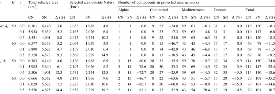
Outputs from the two types of networks (climate and simple networks) obtained under different parameter-izations (e9H9Bi) showed marked variability on the extent (Table1), effectiveness (Fig. 3) and spatial location (Fig.4, and Table S5.1 in the Supplementary material) of linkages connecting the Iberian protected areas. While climate networks ranged from 5,328 to 6,666 km2, simple networks varied from 4,873 to 6,373 km2. This means that climate networks required 3.2–14.4% more area than simple networks, and also identified more linkages outside the Natura 2000 network (3.8–19.2% more area). Models penalizing the number of cells and the total area in the solution (e=0.5) retrieved more distinct solutions between the approaches; a trend that is true for bothH=50 andH=60 scenarios (Table1).
As expected, climate networks performed better in terms of avoiding climatic barriers than equiva-lent simple networks. In fact, by identifying and bypassing climatic barriers, climate networks included 6.0–35.2% less protected area components than simple networks, a fact that is contingent on the spatial pattern of unsuitable areas provided byHand Bi. Differences in the number of components vary with the climatic classes, because linkages between
protected areas in particular classes are more challenged by barriers.
When barriers included the 25% more dissimilar cells outside protected areas of each type [Bi[Q3 di(s)], greater differences between the climate and simple networks were obtained for the alpine pro-tected area network (Table1). With climate networks, linkages for these protected areas retrieved few components (2–3) being 72.7–86.7% more effective at guaranteeing connectivity than linkages in the simple networks. TurningH=50 toH=60 greatly affected comparisons of both approaches for the continental protected areas, as effectiveness gains with climate networks varied approximately from 30 to 60%. This means that the general (landscape) barriers are the major determinant of fragmentation for these protected areas. Differences between approaches were less marked when connecting Mediterranean and oceanic protected areas, with gains in effectiveness being approximately 15% for climate networks. Using H=50, effectiveness gains in oceanic protected areas were narrower (3.0–5.9%).
Comparing efficiency and effectiveness of climate and simple networks enables the assessment of the extent to which a fixed budget produces solutions performing differently in terms of realized linkage achievements. Climate networks are inevitably more costly than simple networks when the same parame-terization is used. Therefore, we manipulated area-penalty to obtain climate and simple networks with similar costs. For example, analysing the more Fig. 2 The effect of changing parameters over the linkage
solutions, using a synthetic example where three habitat units (A,BandC) are to be linked.aThe barrier effect (landscape and environmental barriers). When barriers (circles) do not isolate sets of habitats thegrey cellsare a likely solution to connectA,B
andC. Otherwise, when barriers (crossed-cells) isolate sets of habitats, a linkage is only required to connectBandC(
thick-bordered white cells), whileAstays isolated;bThe effect of the
area-penalty value, epsilon (e). Whene\0.2, the ‘‘cheapest’’ connection is the one passing through the 20 thick-bordered
zero-cost white cells(total cost=209e). Whene[0.2, the
cheapest connection is the one passing through thegrey cells
Table 1 Summary of networks of Iberian protected areas, obtained with climate data (climate networks; CN) and without climate data (simple networks; SN) using different
parameterizations of the human footprint thresholdH, the area-penalty parametere, and climatic barriersBi
Bi H e Total selected area
(km2)
Selected area outside Natura (km2)
Number of components in protected area networks
Alpine Continental Mediterranean Oceanic Total
CN SN D(%) CN SN D(%) CN SN D(%) CN SN D(%) CN SN D(%) CN SN D(%) CN SN D(%)
max di 50 0.0 6,361 6,140 3.6 2,083 1,988 4.8 1 1 0.0 19 25 -24.0 59 63 -6.3 31 31 0.0 110 120 -8.3
0.1 5,934 5,639 5.2 2,163 2,026 6.8 1 1 0.0 19 23 -17.3 59 62 -4.8 31 31 0.0 110 117 -6.0
0.5 5,331 4,901 8.8 2,473 2,244 10.2 1 1 0.0 19 25 -24.0 59 63 -6.3 31 31 0.0 110 120 -8.3
60 0.0 6,577 6,373 3.2 2,034 1,959 3.8 1 1 0.0 8 15 -46.7 43 45 -4.4 17 17 0.0 69 78 -11.5
0.1 5,890 5,622 4.7 2,138 2,010 6.4 1 1 0.0 8 14 -42.9 43 46 -6.5 17 17 0.0 69 78 -11.5
0.5 5,328 4,873 9.3 2,562 2,229 14.9 1 1 0.0 8 13 -38.5 43 45 -4.4 17 17 0.0 69 76 -9.2
Q3di 50 0.0 6,383 6,140 4.0 2,126 1,988 6.9 3 15 -80.0 20 31 -35.5 59 70 -15.7 32 34 -5.9 114 150 -24.0
0.1 5,985 5,640 6.1 2,193 2,026 8.2 3 14 -78.6 20 30 -33.3 59 69 -14.5 32 34 -5.9 114 147 -22.4
0.5 5,506 4,901 12.3 2,531 2,244 12.8 3 11 -72.7 20 27 -25.9 59 69 -14.5 32 33 -3.0 114 140 -18.6
60 0.0 6,666 6,362 4.8 2,143 1,956 9.6 2 15 -86.7 8 22 -63.6 43 51 -15.7 17 20 -15.0 70 108 -35.2
0.1 6,029 5,622 7.2 2,223 2,010 10.6 2 14 -85.7 8 20 -60.0 43 53 -18.9 17 20 -15.0 70 107 -34.6
0.5 5,576 4,875 14.4 2,657 2,229 19.2 2 11 -81.1 8 17 -52.9 43 54 -20.4 17 19 -10.5 70 101 -30.7
Percentage-differences [D(%)] between CN and SN are presented for the total selected area, the selected area outside Natura 2000 network, the total number of protected area
components and for the number of components within each of the climatic classes (alpine, continental, Mediterranean and oceanic)
Landscape
Ecol
(2012)
27:291–301
297
conservative scenario (i.e., with more barriers) [H=50, Bi[Q3 di(s)], the climate networks requiring less surface area targeted 5,506 km2, encom-passing 114 protected area components, while a similar-size simple networks (5,640 km2) contained 147 protected area components (Fig.3a). An equiv-alent loss of linkage effectiveness for the simple networks occurred when the selected area outside Natura 2000 was used as a measure of efficiency (Fig.3b). In this case the most-costly simple network (2,244 km2) presented more 22.8% protected areas components than the climate network using a similar amount of area outside Natura 2000 (2,193 km2). These differences are directly translated to the spatial patterns obtained for both network types (Fig.4).
Discussion
We have shown that extending the MST to account for different types of terminal habitats provides a useful framework for identifying linkages between natural areas using environmental data. The framework is based on the assumption that the environment drives, at least partially, species’ distributions, so that habitats with similar environments are likely to share similar assemblages of species or act as potential ‘sources’ and ‘sinks’ for species’ dispersal. It follows from this assumption that linkages between protected areas should preferentially be established between environ-mentally-similar areas. Although this assumption is problematic for the selection of complementary sets of Fig. 3 Comparison of networks delineated with climate data
(climate networksCN) (filled squares) with simple networks without climatic data (simple networksSN) (open circles) in terms of efficiency:aTotal area selected,bTotal area selected not listed in Natura 2000; and effectiveness (number
components in protected area networks), for the most conser-vative scenario under consideration [H=50,Bi[Q3 di(s)], using distinct area-penalty parameterizations (e values in
parenthesis).Arrowsrepresent comparisons of pairs of networks
sharing similar costs
Fig. 4 Maps of linkages for the Iberian Peninsula protected areas obtained with climate data (climate networksCN), using an area-penaltye=0.1 and climatic barriersBi[Q3di(s), and without climate data (simple networksSN) using an area-penalty e=0.5. Both networks are delineated over a similar amount of
areas in reserve selection (see, Arau´jo et al. 2001; Arau´jo et al.2004; Hortal et al.2009), it is reasonable to expect that when species occupying a given environment are, for whatever reason, forced to move elsewhere, they preferentially move to similar envi-ronments (Chetkiewicz et al. 2006; Sawyer et al. 2011). The choice of the relevant environmental attributes to be used should be concerted with the autoecology of focal species and the scale of analysis (i.e., extent and resolution of the study area). For example, we used climate to obtain a broad charac-terization of species’ permeability in Iberian Peninsula as it is seen highly correlated with plant and animal species’ distributions at such spatial extent and grain size (Hawkins et al. 2003; Whittaker et al. 2007). Several other environmental variables could be used instead (e.g., vegetation types, topography, geology, biogeography, phylogeny and disturbance data, or different combinations of them).
Two problems may arise when using climatic variables in our framework in a context of climate change. First, sets of climatically-similar habitats are likely to be shuffled with climate change and therefore an habitat unit A initially targeted to be linked with a similar unit B, may no longer need such linking, but requires a linkage with a new similar unit C. Second, areas identified as linkages for a given habitat class may lose climatic suitability for that class. In an extreme scenario, they may even turn into barriers to species’ movements. To develop conservation maps robust to climate change (without relying on projected emissions of greenhouse gases, air-ocean circulation models, and climate-envelope models), several studies support the use of more steady factors driving biodiversity patterns and processes, like topographic and geomorphologic variation (Anderson and Ferree 2010; Beier and Brost2010; Game et al.2011).
Our framework is flexible enough to accommodate simple conservation purposes. For example, natural habitats may be so heavily fragmented that no continuous swaths of land are left to be conserved. Furthermore, there are species able to cross some amount of inhospitable land. In cases such as these, linking habitats with stepping-stones may open oppor-tunities for effective and less-conflicting conservation measures, because stepping stones require lesser area than continuous linkages. Our framework may be easily adapted to delineate stepping-stones optimally. This can be accomplished by using adjacency rules
between cells that integrate a ‘‘functional distance’’ defined by the distance that the least mobile focal species are able to move across unsuitable habitat. Once a given cell is chosen for linkage at least one other cell, distancing no more than the ‘‘functional distance’’, needs also to be selected.
The cost-optimised networks obtained with our framework only require a unique path between each pair of habitat units of the same class. This may not be the most precautionary option to take (Pinto and Keitt 2009). One can increase network robustness by identifying multiple paths to link habitats of the same class. Our framework is able to reach this by replacing the execution of the last step of the linkage algorithm (i.e., turning the solution minimal), with the removal of only the non-terminal cells that are connected to no more than one other cell. Then, if non-overlapping linkages are desired, the heuristic can be repeatedly run removing all the selected non-terminal cells from the previous solutions. Clearly, this can be executed only for those habitat classes with greater numbers of threatened species or for the classes requiring longer linkages, as these are less likely to be implemented or are more exposed to threats (Beier and Noss 1998). Furthermore, in circumstances where lengthy linkages are not critical to maintain long distance dispersal events, it may be wiser to avoid linking distant habitat units. For example, the analysed region may be sub-divided in order to obtain sub-areas with higher densities of habitat units for each habitat class. Independent solutions for each of these sub-areas may be obtained thereafter.
Finally, it is critical to realize that if the main interest of conservation is the persistence of species in fragmented landscapes, the sole integration of species’ movement patterns is insufficient. Species’ dispersal data should be combined with other factors that determine species’ persistence at various spatial and temporal scales. The framework here presented should be considered as part of a broader analysis towards the promotion of such complex and integrative objective as it is allowing species to persist.
Acknowledgments DA was supported by a PhD studentship (BD/27514/2006) and is now funded by a post-doctoral fellowship (BPD/51512/2011) awarded by the Portuguese Foundation for Science and Technology (FCT); MT is funded by a FPI-MICINN (BES-2007-17311) fellowship; MC was funded through a Spanish RyC fellowship; JOC is partially supported by FCT through the European Community Fund
FEDER/POCI 2010 and by the FCT project PTDC/AAC-AMB/ 113394/2009; MBA is currently funded by the ECOCHANGE project and acknowledges support from the Rui Nabeiro/Delta Chair in Biodiversity and the Spanish Research Council (CSIC). We are grateful to Evgeniy Meyke for the treatment of Iberian Peninsula Natura 2000 data.
References
Aarts EHL, Korst JHM, van Laarhoven PJM (1997) Simulated annealing. In: Aarts E, Lenstra JK (eds) Local search in combinatorial optimization. Wiley, New York, pp 91–120 Alagador D, Cerdeira JO (2007) Designing spatially-explicit reserve networks in the presence of mandatory sites. Biol Conserv 137:254–262
Anderson MG, Ferree CE (2010) Conserving the stage: climate change and the geophysical underpinnings of species diversity. PLoS ONE 5:e11554
Arau´jo M (2009) Climate change and spatial conservation planning. In: Moilanen A, Possingham H, Wilson KA (eds) Spatial conservation prioritization: quantitative methods and computational tools, Oxford University Press, Oxford, pp 172–184
Arau´jo MB, Humphries CJ, Densham PJ, Lampinen R, Hage-meijer WJM, Mitchell-Jones AJ, Gasc JP (2001) Would environmental diversity be a good surrogate for species diversity? Ecography 24:103–110
Arau´jo MB, Densham PJ, Williams PH (2004) Representing species in reserves from patterns of assemblage diversity. J Biogeogr 31:1037–1050
Arau´jo MB, Alagador D, Cabeza M, Nogue´s-Bravo D, Thuiller W (2011a) Climate change threatens European conserva-tion areas. Ecol Lett 14:484–492
Arau´jo MB, Guilhaumon F, Neto DR, Pozo I, Calmaestra RG (2011b) Impactos, vulnerabilidad y adaptacio´n al cambio clima´tico de la biodiversidad espan˜ola, 2nd edn. Fauna de Vertebrados, Madrid
Baldwin RF, Perkl R, Trombulak S, Burwell W (2010) Mod-eling ecoregional connectivity. In: Trombulak S, Baldwin RF (eds) Landscape-scale conservation planning. Springer-Verlag, Dordretch
Beier P, Brost B (2010) Use of land facets to plan for climate change: conserving the arenas, not the actors. Conserv Biol 24(3):701–710
Beier P, Noss R (1998) Do habitat corridors provide connec-tivity? Conserv Biol 12:1241–1252
Beier P, Spencer W, Baldwin RF, McRae BH (2011) Toward best practices for developing regional connectivity maps. Conserv Biol 25:879–892
Bull JC, Pickup NJ, Pickett B, Hassell MP, Bonsall MB (2007) Metapopulation extinction risk is increased by environ-mental stochasticity and assemblage complexity. Proc R Soc B Biol Sci 274:87–96
Butchart SHM, Walpole M, Collen B, van Strien A, Scharle-mann JPW, Almond REA, Baillie JEM, Bomhard B, Brown C, Bruno J, Carpenter KE, Carr GM, Chanson J, Chenery AM, Csirke J, Davidson NC, Dentener F, Foster M, Galli A, Galloway JN, Genovesi P, Gregory RD,
Hockings M, Kapos V, Lamarque J-F, Leverington F, Loh J, McGeoch MA, McRae L, Minasyan A, Morcillo MH, Oldfield TEE, Pauly D, Quader S, Revenga C, Sauer JR, Skolnik B, Spear D, Stanwell-Smith D, Stuart SN, Symes A, Tierney M, Tyrrell TD, Vie´ J-C, Watson R (2010) Global biodiversity: indicators of recent declines. Science 328:1164–1168
Calabrese JM, Fagan WF (2004) A comparison-shopper’s guide to connectivity metrics. Front Ecol Environ 2:529–536 Cerdeira JO, Gaston KJ, Pinto LS (2005) Connectivity in
pri-ority area selection for conservation. Environ Model Assess 10:183–192
Cerdeira JO, Pinto LS, Cabeza M, Gaston KJ (2010) Species specific connectivity in reserve-network design using graphs. Biol Conserv 143:408–415
Chetkiewicz CLB, Boyce MS (2009) Use of resource selection functions to identify conservation corridors. J Appl Ecol 46:1036–1047
Chetkiewicz C-LB, St. Clair CC, Boyce M (2006) Corridors for conservation: integrating pattern and process. Annu Rev Ecol Evol Syst 37:317–342
Conrad J, Gomes CP, van Hoeve W-J, Sabharwal A, Suter JF (2010) Incorporating economic and ecological information into the optimal design of wildlife corridors, Cornell Uni-versity, Ithaca
Dijkstra EW (1959) A note on two problems in connexion with graphs. Numer Math 1:269–271
Du D, Hu X (2008) Steiner tree problems in computer com-munication networks, World Scientific Publishing Co Pte Ltd., Singapore
Fahrig L, Merriam G (1994) Conservation of fragmented pop-ulations. Conserv Biol 8:50–59
Fielding AH (2007) Cluster and classification techniques for the biosciences. Cambridge University Press, Cambridge Fischer DT, Church RL (2003) Clustering and compactness in
reserve site selection: an extension of the biodiversity management area selection model. For Sci 49:555–565 Fuller T, Sarkar S (2006) LQGraph: a software package for
optimizing connectivity in conservation planning. Environ Model Softw 21:750–755
Fuller T, Munguia M, Mayfield M, Sanchez-Cordero V, Sarkar S (2006) Incorporating connectivity into conservation planning: a multi-criteria case study from central Mexico. Biol Conserv 133:131–143
Game ET, Lipsett-Moore G, Saxon E, Peterson N, Sheppard S (2011) Incorporating climate change adaptation into national conservation assessments. Glob Change Biol 17:3150–3160 Hannah L, Midgley GF, Andelman S, Arau´jo MB, Hughes G, Martinez-Meyer E, Pearson RG, Williams PH (2007) Protected area needs in a changing climate. Front Ecol Environ 5:131–138
Hanski I (1999) Habitat connectivity, habitat continuity, and metapopulations in dynamic landscapes. Oikos 87:209–219 Hawkins BA, Field R, Cornell HV, Currie DJ, Gue´gan J-F, Kaufman DM, Kerr JT, Mittelbach GG, Oberdorff T, O’Brien EM, Porter EE, Turner JRG (2003) Energy, water, and broad-scale geographic patterns of species richness. Ecology 84:3105–3117
IUCN (2010) IUCN red list of threatened species. Version 2010.1 IUCN
Kruskal JB (1956) On the shortest spanning subtree of a graph and the traveling salesman problem. Proc Am Math Soc 7:48–50
McDonnell MD, Possingham HP, Ball IR, Cousins EA (2002) Mathematical methods for spatially cohesive reserve design. Environ Model Assess 7:107–114
O¨ nal H, Briers RA (2002) Incorporating spatial criteria in optimum reserve network selection. Proc R Soc Lond B Biol Sci 269:2437–2441
O¨ nal H, Briers RA (2003) Selection of a minimum-boundary reserve network using integer programming. Proc R Soc Lond B Biol Sci 270:1487–1491
O¨ nal H, Briers RA (2005) Designing a conservation reserve network with minimal fragmentation: a linear integer pro-gramming approach. Environ Model Assess 10:193–202 O¨ nal H, Wang Y (2008) A graph theory approach for designing
conservation reserve networks with minimal fragmenta-tion. Networks 51:142–152
Peel MC, Finlayson BL, McMahon TA (2007) Updated world map of the Ko¨ppen-Geiger climate classification. Hydrol Earth Syst Sci 11:1633–1644
Pinto N, Keitt T (2009) Beyond the least-cost path: evaluating corridor redundancy using a graph-theoretic approach. Landscape Ecol 24:253–266
Prim RC (1957) Shortest connection networks and some gen-eralizations. Bell Syst Tech J 36:1389–1401
Rayfield B, Fortin M-J, Fall A (2011) Connectivity for conser-vation: a framework to classify network measures. Ecology 92:847–858
Rothley KD (1999) Designing bioreserve networks to satisfy multiple, conflicting demands. Ecol Appl 9:741–750 Sanderson EW, Jaiteh M, Levy MA, Redford KH, Wannebo
AV, Woolmer G (2002) The human footprint and the last of the wild. Bioscience 52:891–904
Saura S, Pascual-Hortal L (2007) A new habitat availability index to integrate connectivity in landscape conservation planning: comparison with existing indices and application to a case study. Landsc Urban Plan 83:91–103
Sawyer SC, Epps CW, Brashares JS (2011) Placing linkages among fragmented habitats: do least-cost models reflect how animals use landscapes? J Appl Ecol 48:668–678 Sessions J (1992) Solving for habitat connections as a Steiner
network problem. For Sci 38:203–207
Taylor PD, Fahrig L, Henein K, Merriam G (1993) Connectivity is a vital element of landscape structure. Oikos 68:571–573 Theobald D (2010) Estimating natural landscape changes from 1992 to 2030 in the conterminous US. Landscape Ecol 25:999–1011
Urban D, Keitt T (2001) Landscape connectivity: a graph-the-oretic perspective. Ecology 82:1205–1218
Whittaker RJ, Nogue´s-Bravo D, Arau´jo MB (2007) Geograph-ical gradients of species richness: a test of the water-energy conjecture of Hawkins et al. (2003) using European data for five taxa. Glob Ecol Biogeogr 16:76–89
Williams JC (1998) Delineating protected wildlife corridors with multi-objective programming. Environ Model Assess 3:77–86
Williams JC (2002) A zero-one programming model for con-tiguous land acquisition. Geogr Anal 34:330–349 Williams JC, ReVelle CS (1998) Reserve assemblage of critical
areas: a zero-one programming approach. Eur J Oper Res 104:497–509
Williams J, ReVelle C, Levin S (2005) Spatial attributes and reserve design models: a review. Environ Model Assess 10:163–181
Wu X, Murray A, Xiao N (2011) A multiobjective evolutionary algorithm for optimizing spatial contiguity in reserve net-work design. Landscape Ecol 26:425–437