ON RECOV ERY AN D I N TEN SI TY’S CORRELATI ON
- A N EW CLASS OF CRED I T RI SK M OD ELS*
Raquel M. Gaspar, Advance Research Cent er, I SEG, Technical Universit y Lisbon
E- m ail: Rm [email protected] l.pt
I rina Slinko, Group Risk Cont rol
Swedbank AB
E- m ail: ir ina.slinko@sw edbank.se
W ORKI N G PAPER N . 1 / 2 0 0 7
July 2007
Abst r a ct
There has been increasing support in t he em pirical lit erat ure t hat bot h t he probabilit y of default ( PD) and t he loss giv en default ( LGD) are correlat ed and driven by m acroeconom ic variables. Paradoxically, t here has been very lit t le effort from t he t heoret ical lit erat ure t o develop credit risk m odels t hat would include t his possibilit y. The goals of t his paper are: first , t o develop t he t heoret ical reduced- form fram ework needed t o handle st ochast ic correlat ion of recovery and int ensit y, proposing a new class of m odels; and, second, t o use concret e inst ance of our class t o st udy t he im pact of t his correlat ion in credit risk t erm st ruct ures. Our class of m odels is able t o replicat e and explain em pirically observed feat ures. For inst ance, we aut om at ically get t hat periods of econom ic depression are periods of higher default int ensit y and where low recovery is m ore likely - t he well- know credit risk business cycle effect . Finally, w e show how t o calibrat e t his class of m odels t o m arket dat a, and illust rat e t he t echnique using our concret e inst ance using US m arket dat a on corporat e yields.
Ke y w or ds: Credit Risk; Syst em at ic Risk; I nt ensit y Models; Recovery; Credit Spreads.
JEL Cla ssifica t ion: C15, G12, G13, G33
_ _ _ _ _ _ _ _ _ _ _ _ _ _ _ _ _
* We gr at efully acknow ledge financial suppor t fr om Jan Wallander and Tom Hedelius foundat ion. This
r esear ch w as also par t ially suppor t ed by t he Aust r ian Science Foundat ion pr oj ect P18022 at t he Vienna Universit y of Technology
1
Introduction
Recent empirical studies show that there is a significant systematic risk component in default-able credit spreads. See Altman, Resti, and Sironi (2004), D¨ullmann and Trapp (2000), Elton and Gruber (2004), Frye (2000a) or Frye (2003). The model underlying the Basel II internal ratings-based capital calculation – see Basel Committee (2003) and Wilde (2001) – measures credit portfolio losses only, that is, portfolio losses that are due to external influences and hence cannot be diversified away. This gives us an indication of what the main concerns are in practice and highlights the need for a realistic model ofsystematic risk.
Both the probability of default (PD) and the loss given default (LGD) are key in accessing expected capital losses and measuring the exposure of portfolios of defaultable instruments to credit risk. In accessing capital at risk, it is extremely important not to ignore the interdepen-dence between PD and LGD, since this could lead to underestimation of the true risk borne by portfolio holders. In fact, there has been increasing support on the empirical literature agreeing on two observed facts: (i) PD and LGD are correlated and (ii) macroeconomic risks are likely to affect both these variables. See Allen and Saunders (2003), Altman, Braddy, Resti, and Sironi (2005), Frye (2000b), Giese (2005) or Hu and Perrandin (2002). Nonetheless, most of the theoretical literature considers models where only the default intensity, or equivalently the PD, is dependent on a state variable assuming that the LGD is either fixed or at least independent of default intensities. See Wilson (1997), Saunders (1999), JP Morgan (1997), Gordy (2000), or Sch¨onbucher (2001).
The purpose of this study is to, based on the theoretical flexibility of DSMPP, present a reduced-form multiple default family of models that considers the influence of macroeconomic risks on
both PD and LGD. This leads to the first theoretical family of models that is able to reproduce the empirical facts stated above, i.e., allows for correlated PD and LGD and considers the influence of systematic risks on both variables. The final goal is then to see if including these facts in the theoretical framework will help in explaining observed behavior of the term structure of credit spreads.
As a proxy for macroeconomic conditions we consider a market index. It is well known that market uncertainty and its level are negatively correlated. That is, periods of recession (low index level) also tend to be periods of high uncertainty (high index volatility) reflecting some sort of market panic, while periods of economic boom are perceived as safe periods and with low uncertainty. In setting up the dynamics of the market index, we incorporate this realistic feature by allowing the local volatility of the index to depend negatively on its level.
In terms of the PD and LGD, we assume that default intensity and the recovery given default depend on the market situation (the index level). With the PD dependence we try to account for the fact that during recessions it is reasonable to expect more defaults, while with the LGD dependence we try to account for the fact that if the entire market is down, the market value of any firm’s assets should be lower, and debt holders should recover less if a default occurs.
The main contributions of this study can be summarized as follows.
• We suggest a multiple default reduced-form model where we use the flexibility of DSMPP to model the influence of systematic risks on both PD and LGD.
• We derive general qualitative impacts of the macroeconomic risks, on intensity of default, recovery given default and credit spreads, that should hold in realistic theoretical models.
the term structure of credit spreads, showing that the correlation between PD and LGD (resulting from the influence of the systematic risk) must be considered.
• Finally, we show how to calibrate our model to market data.
The rest of the paper is organized as follows. In Section 2 we setup the framework and summa-rize the main theoretic results concerning the use of DSMPP in credit risk models. In Section 3 we propose a family of macroeconomic models, presenting the index dynamics and justifying the assumptions about the influence of such risks on the intensity and recovery processes using empirical facts. We derive qualitative results on the influence of the market index on default intensity, recovery and credit spreads. In Sections 4 we present a concrete instance of our class of models simulate it to access the impacts of our qualitative assumptions in terms credit spread term structures. We end the section discussion calibration issues of models with no closed-form solution and calibrate our own concrete model US market data. Section 5 concludes the paper, summarizing the main results and suggesting directions for future research.
2
The setup and fundamental theoretic results
We consider a financial market living on a filtered probability spaceΩ,F,Q,(Ft)0≤t≤T
where
Q is the risk-neutral probability measure. The probability space carries a multidimensional Wiener process W and, in addition, a doubly stochastic marked point process (DSMPP),
µ(dt, dq), on a measurable mark space (E,E) to model the default events. The filtration (Ft)0≤t≤T is generated byW andµ, i.e. Ft=FtW ∨ F
µ t .
2.1
Default-free bond market
We assume the existence of a liquid market for default-free zero-coupon bonds, for every possible maturity T. We denote the price at time t of a default-free zero-coupon bond with maturity
T byp(t, T). The instantaneous forward rate with maturityT is denotedf(t, T) and we recall one-to-one correspondence between zero-coupon bond prices and forward rates:
f(t, T) =−∂lnp(t, T)
∂T ⇔ p(t, T) = exp
(
−
Z T
t
f(t, s)ds
)
. (1)
The default-free short rate is denotedr(t) =f(t, t).
2.2
Defaultable bond market
In addition to the risk-free bond market mentioned above, we consider a defaultable bond market. We assume that each company on the market issues a continuum of bonds with maturitiesT. Assumption 2.1 and Assumption 2.3 below characterize the default events and the dependence of both the default intensity and the recovery rate distribution on an abstract stochastic state variableX.
Assumption 2.1.There exist an underlying stochastic state variableX, whose dynamics under
the risk neutral measureQis given by
In our framework we will allow for multiple defaults. Behind this is the intuition that, given a distress situation for the obligator’s business, the debt holders are willing to accept the renegotiation of their claims (accepting to lose some fractionq of the face value of the claims) in order to avoid a process of bankruptcy, which is typically costly, and allowing the firm to continue operating.1 It is possible that a whole sequence of defaults is taking place, every time
leading to reduction of the debt’s face value and the bondholder accepting the conditions of the deal.
We now define the key notions for the defaultable bond market and formalize the assumptions concerning the occurrence of default events.
Definition 2.2. (Basic Definitions)
• Theloss quota is the fraction by which the promised final payoff of the defaultable claim is reduced at each time of default. We denote the loss quota by q.
• Theremaining value, after all reductions in the face value of the defaultable claim due to defaults in the time interval [0, t], is denotedV(t).
• p¯(t, T) is, at time t, theprice of a defaultable zero-coupon bond with maturityT and the face value 1. The payoff at time T of the bond is, thus, V(T) the remaining part of the face value of the bond after all reductions due to defaults in the time interval [0, T], i.e.,
¯
p(T, T) =V(T).
• We define the instantaneous defaultable forward rate, ¯f(t, T), similarly to its risk-free equivalent, we have ¯p(t, T) =V(t) expn−RtTf¯(t, s)dsoand ¯f(t, T) =− ∂
∂Tln ¯p(t, T).
• Thedefaultable short rate is defined as ¯r(t) = ¯f(t, t).
• Theshort credit spread s(t) is defined as the difference between the defaultable and non-defaultable short ratess(t) = ¯r(t)−r(t).
• Theforward credit spread s(t, T) is defined as the difference between the defaultable short rate and non-defaultable forward rates,s(t, T) = ¯f(t, T)−f(t, T).
Assumption 2.3. (Default Events)
1. We assume that default happens at the following sequence of the stopping timesτ1< τ2<
. . ., whereτi is the time of thei-th jump of a point process.
2. At each default timeτi the loss quotaqi is drawn from the mark space E= (0,1).
3. We assume that there is no total loss at default, i.e., the loss quota qi <1 for all i =
1,2,· · ·.
4. We assume that both:
(i) the arrivals of default times(τi)i≥1;
(ii) the distribution of the loss quotas given default (qi)i≥1
depend upon the stochastic state processX.
1Multiple default models mimic the effect of a rescue plan as it is described in many bankruptcy codes. The
Given that at each default timeτithe final claim amount is reduced by a loss quotaqito (1−qi)
times what it was before, we obtain
V(t) = Y
τi≤t
(1−qi), (3)
whereqi is the stochastic marker to the default timeτi. Obviously, in case of no default on the
interval [0, T],V(t) = 1.
2.2.1 The default process
We start by giving the abstract definition of a Marked Poisson Point Process and a Doubly Stochastic Marked Poisson Process (DSMPP). We introduce first the following filtrations.
Notation 1. (Filtrations)
• The filtration generated byW(t), FW t
t≥0, is thebackground filtration. 2
• The filtration GW = _ t≥0
FW
t contains all future and past information on the background
processW .
• Thefull filtrationis reached by combining FW t
t≥0and the filtration (F
µ
t)t≥0, is
gener-ated by MPPµ,Ft =FtW ∨ Ftµ.
• Finally,GW
t =GW∨ F µ
t, is the filtration generated byall the information concerning the
background processW, and only past information on the MPPµ.
Definition 2.4. (DSMPP)
• We call the Marked Point Process ˆµ an Ftµ- Marked Poisson Process if there exists a deterministic measure ˆν onR+×E such that
P(ˆµ((s, t]×B) =k|Fµ s) =
(ˆν((s, t]×B))k
k! e
−νˆ((s,t]×B), a.s., B∈E.
• We call the Marked Point Process µ anGW
t - DSMPP if there exists a GW-measurable
random measureν onR+×E such that
P µ((s, t]×B) =kGW s
=(ν((s, t]×B))
k
k! e
−ν((s,t]×B), a.s., B∈E.
We note that the previous literature on credit risk have only used Doubly Stochastic Poisson process (also known as Cox Processes).3 The focus has been in modeling the jump intensity
λand recovery has been assumed independent ofλ. In factor models the state variable would influence only theλ.
2In our setup, all the default-free processes are adapted to FW t
t≥0.
3We recall that a counting processN= (Tn) adapted to right-continuous filtration is aGW
t - Cox Process if
there is anGW-measurable random measureν satisfying
PN(s, t] =kGsW
= (ν((s, t]))
k
k! e
As far as we know this study is the first using doubly stochasticmarkedpoint processes in credit risk. Our goal is to consider that both intensity and recovery can be affected by a common state variable. For that we need to model the default events using aGW
t -DSMPP whose compensator
depends the Wiener driven stochastic state variableX presented in (2).
An important result for what follows is the existence of such processes, that is DSMPP with a compensator equal to a given random measure, Mt(dq, Xt), and that can be written as a
deterministic function of our state variable. Due to its rather technical level we present the proof of the next Theorem in the appendix.
Theorem 2.5. Assume that a random measureν onR+×Eadmits representationMt(dq, Xt)dt,
whereMt(dq, x)is a deterministic measure on E for any fixedx andt.
Letνˆ(dt, dq) =mt(dq)dt be a deterministic compensator for some Marked Poisson Process µˆ.
Assume that:
(i) Mt(dq, x)is measurable w.r.t. GW
(ii) Mt(dq, x)is absolutely continuous w.r.t. m(t, dq)onE, that is,
Mt(dq, x)<< mt(dq)
Then, there exists a GW
t -DSMPPµ, such that its compensator is of the form
ν(dt, dq, ω) =ν(dt, dq, Xt) =Mt(dq, Xt)dt, Q−a.s. (4)
Given existence of DSMPP, we can now focus the the compensator’s construction. Ideally we would like to model the intensity of default λ(t, Xt) and the instantaneous conditional loss
quota distribution K(t, dq, Xt), separately allowing both those quantities to depend on the
state varibaleX, and not to model the compensatorν(dt, dq, Xt) at once. We propose what we
consider to be a good construction procedure and then justify why it works.
Remark 2.6. (Construction procedure)We construct the DSMPPµ as follows.
1. We specify the Wiener driven stochastic state variableX.
2. We specify the intensityλ(t, Xt)as a function of the state variable.
3. We specify the instantaneous conditional loss quota distribution as a function of the state variable K(t, dq, Xt). 4
4. Finally, we construct the stochastic compensatorν
ν(dt, dq, Xt) =K(t, dq, Xt)λ(t, Xt)dt . (5)
This construction does work because the multiplication of the two quantitiesK(t, dq, Xt) and
λ(t, Xt) is a random measure on R+×E (see, for example, Last and Brandt (1995)). This
together with the result of Theorem 2.5 assures us that, for any given distribution of the loss quota given defaultK(t, dq, Xt) and given intensityλ(t, Xt), there exist aGtW-DSMPP, whose
compensator can be written as in (5).
4In all the practical applications we suppose the instantaneous conditional loss quota distributionsK(t, dq, Xt)
are absolutely continuous with respect to Lebesgue measure onE, that is, we consider conditional loss quota distributions of the formK(t, dq, Xt) = ˜K(t, q, Xt)dq, thusMt(dq, x)<< dq. This is enough to cover all the
The possibility to construct the quantitiesλ(t, Xt) andK(t, dq, Xt) separately has the additional
advantage of satisfying a consistency requirement needed in any credit risk model. That is, we can derive consistently prices, or other credit risk relevant values, that depend exclusively upon default intensity (like the implied survival probability, the price default digital payoffs or the price defaultable bonds with zero recovery) and that depend on both intensity and recovery (like credit default swaps, recovery swaps, or defaultable bonds with non zero recovery).
2.2.2 Fundamental theoretic results
In this section we state the main results on the short and forward credit spreads. The proof of the next Proposition can be found in the appendix.
Proposition 2.7. Given Assumption 2.3, and under the martingale measure Q.
1. The short credit spreads, s(t), have the following functional form
s(t) =λ(t, Xt)qe(t, Xt)>0 (6)
where
qe(t, Xt) =
Z 1
0
qK(t, dq, Xt)
can be interpreted as the locally expected loss quota (which is positive for q >0).
2. Then the forward credit spread s(t, T)takes the form
s(t, T) =
EQt h
{r(T) +λ(T, XT)qe(T, XT)}e−
RT
t {r(s)+λ(s,Xs)qe(s,Xs)}ds
i
EQt he−RT
t {r(s)+λ(s,Xs)qe(s,Xs)}ds
i −f(t, T) (7)
3. The bond prices can be written as
¯
p(t, T) =V(t)EtQhe−RtTr¯sds
i
. (8)
We end up this section with a small remark concerning the modeling choice of the risk-neutral measureQand its consequences in term of the objective probability measureP.
Remark 2.8. (P considerations)
Our setup has been defined under the martingale measure Q. It is possible to show that if the market price of jump risk φis a deterministic function of time then:5
1. TheQ-default intensity, λ, relates to theP-default intensityλP, by
λP(t, X) =λ(t, X)(1 +φ(t)) (9)
2. TheQ-loss quota distribution, conditional on default,Kt(dq, X), equals to the conditional
on default loss quota distribution under P, KP
t (dq, X).
We see that, in this case, the conditional distribution of the loss quota remains unchanged while intensity changes according to (9), i.e. multiplied by a deterministic function of time. The assumption the market price of jump risk is deterministic allows us to use our objective intuitions in setting up the applied model for macroeconomic risks6.
5This result is a direct application of the Girsanov Theorem. Upon request the authors will gladly provide
the exact proof.
3
The Macroeconomic Risks
In this section we discuss the main economic arguments behind our general assumptions. All assumptions that result from empirical facts and economics arguments will be referred to as
properties 7and numbered with roman letters (i), (ii), etc.
We start by modeling the systematic risk of the economy. For that we consider what we call a
market index,I. At all times, we consider both the case when this is the price of an important traded asset (say, oil prices) and the case when it is not the price of any traded asset (e.g. a stock market index).
It has been shown that market index volatility tends to increase when the market as a whole is depressed (low values of the index) and, conversely, volatility decreases when the market index is high, i.e. periods when the market as a whole is depressed are periods of higher volatility, while booms are associated with low volatilities. For example, Jiang and Sluis (1995) show that S&P500 has stochastic volatility. Gaspar (2001) does a comparative study of US and Europe stock markets (using S&P500 and EuroStoxx 50 indices) and shows this feature persists across markets. Selcuk (2005) shows that the innovations to a stock market index and innovations to volatility are negatively related, especially in emerging markets. In order to account for this fact (Property (i)), we consider a local volatility model where index volatility dependent on the index level.
Assumption 3.1. (Market Index)
Under the martingale measure Q, the market index I, satisfies the following stochastic differ-ential equation (SDE)
dIt =ζ(t)Itdt+γ(t, It)ItdW(t),
where γ is a row-vector, W is a Q-Wiener process, and we assume that I is not a price of a
traded asset. If I is a price of a traded asset, we replace ζ by the short rater.
Furthermore, for each entryγi, the following holds
∂γi
∂I(t, I)<0 (i)
It is also reasonable to assume that firms may have different sensitivities to the market index. We, thus, introduce a measure of sensitivity to systematic risk,ǫ,ǫ∈[0,1].
We now discuss the impact one would expect the market indexI to have at default intensities and recoveries of firms.
Assumption 3.2. (The default Intensity)
The intensity is a deterministic function of (t, I, ǫ). Furthermore, we have (¯λ∈R+)
λ(t, I,0) = λ¯ (ii)
∂λ(t, I, ǫ)
∂ǫ > 0 (iii)
∂λ(t, I, ǫ)
∂I < 0 (iv)
We start by noting that if the firm’s financial situation is strong enough, it should not really matter if the economy is booming or if it is in recession. That is, firms that are financially solid
7The same properties (qualitative relations) hold underPandQas long as the market price of jump risk is
should be much less (or not at all) sensitive to the business cycles than those in a less solid financial position. From this point of, the parameterǫ, can be also regarded as a measure of a firm’s credit worthiness. Firms with high credit worthiness typically tend to be less sensitive to the business cycle influence than less credit worthy firms. If this is so, then it makes sense to have properties (ii) and (iii). Property (ii) tells us that the default probability of some firms may be independent of the market situation. Property (iii) says that firms that are more sensitive to the market (have lower credit worthiness) have higher probability of default.
Finally, from Property (iv), we see that, if companies are sensitive to business cycle, then there is higher probability of default during the recession periods (lowI) than in booms (highI).
Assumption 3.3. (Loss Quota)
The conditional distribution of loss quota is a deterministic function of(t, I). K is a stochastic kernel from R+×R+×R+→[0,1]for any realization of(t, I) .
We denote the cumulative distribution function of loss quota conditional on default asK˜
˜
K(t, I, x) = Z x
0
K(t, I, dq),
Z 1
0
K(t, I, dq) = 1, ∀t, I
with the following property, K˜(t, I1, x)≥K˜(t, I2, x) if I1≥I2, ∀x∈R , i.e.,
∂K˜(t, r, I, x)
∂I >0 (v)
∀t,K˜(t, I, x) stochastically dominatesall the conditional distributionsI ≤I.
Property (v) assumes it is more likely, for the loss quota q, to be below some fixed x when index values are low (lowI). Indeed, if a firm is in distress and going to restructure its debt during a recession, its assets are worth less and hence debt holders are more likely to accept a higher loss of their debt face value. Moreover, bankruptcy costs tend to be higher in periods of recession, due to the decreased value of firm’s assets, emphasizing this effect. From the stochastic dominance assumption above, we can now infer the impacts in terms of expected loss quota.
Lemma 3.4. Given Assumption 3.3, the following relations hold for the expected value
qe(t, I) =
Z 1
0
qK(t, I, dq), ∂q
e(t, I)
∂I <0 (vi)
Proof. We obtain the result integrating by parts, differentiating w.r.tI and using (v).
Remark 3.5. (Tractability)
We note that besides the above mentioned properties,K, conditional on the state variable infor-mation, must be the distribution of a random variable taking values in(0,1), and the intensity
λmust be always positive. It is, thus, extremely hard to find a treatable model where these two facts together with properties (i)-(vi) are satisfied. In particular, we have found that no model of affine or quadratic spreads8 will verify all the above properties.
Given these tractability difficulties we go on with the analysis and drawqualitative results of the influence of the market index on credit spreads.
8Outside the class of affine or quadratic spread models it is basically impossible to find closed-form solutions.
Remark 3.6. (Short spread impact)
Given the results in Proposition 2.7, Assumption 3.2 and Lemma 3.4, the short credit spread can be rewritten as a function of(t, , I, ǫ)and
s(t, I, ǫ) =λ(t, r, I, ǫ)qe(t, I) . (10)
Furthermore we have s(t, I,0) = ¯λqe(t, I) , ∂s(t, I, ǫ)
∂ǫ =
∂λ(t, I, ǫ)
∂ǫ
| {z }
>0
qe(t, I)>0 and
∂s(t, I, ǫ)
∂I =
∂λ(t, I, ǫ)
∂I
| {z }
<0
qe(t, I) +λ(t, I, ǫ)∂q
e(t, I)
∂I
| {z }
<0
<0.
We note that, given a concrete functional form for the intensityλand for the loss quota distri-bution the above effects on the short spread in (10) can actually be quantified. Unfortunately, this is not going to be the situation when dealing with forward credit spreads. For the forward credit spreads s(t, T) we obtain expressions in terms of expectations (see Equation (7)) that must be simulated.
4
A concrete model
In this section we illustrate the previous theoretical results using a concrete instance of our class of models. We aim to highlight the importance of considering the dependence between recovery and intensity of default, showing impacts obtained are substantial. We are more concerned with showing the applicability of the results than constructing a extremely realistic (necessary complicated) model. For that reason, our concrete model is as simple as possible. This has the additional advantage of more tractable formulas and a better understanding of what drives the simulation results. The theoretical results apply, of course, more generally many more examples could have been considered.
In order to have a concrete model we need to:
• establish the dependence of the volatility of the index γ, on the index level;
• provide the intensity functional form forλ, in terms of (t, I, ǫ);
• decide on a distribution for the loss quotaq for all possible (t, I).
In the model we take the risk-free rate, r, as constant and abstain from considerations about the term structure of risk-free interest rates. Although unrealistic, it is not harmful to our goal of understanding the impact on spreads. I is assumed to be the price of a traded asset. To consider a non-traded asset, we would need further considerations on the market price of index risk. For simplicity we also take all functions to be time homogenous; the extension to non-time homogeneous functions is straightforward. Given these simplifications, and to have a completely specified model to simulate, we need to define a functionγ(I) for the index volatility, a functionλ(I, ǫ) for the intensity, and a distribution functionK(dq, I) for the loss quota.
We start by defining a ratio, m, which relates the current value of the index to its long-run trend value. Let us define
m(I) =I¯
I,
0 1 2 3 4 5 0.14
0.16 0.18 0.2 0.22 0.24 0.26
0 1 2 3 4 50.5
1 1.5 x 10⁴
0 1 2 3 4 50.8
0.9 1 1.1 1.2 1.3 1.4 x 10⁴
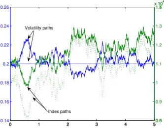
Index paths Volatility paths
Figure 1: Two paths for the index level and volatility. The same noise was used for both cases, and we took ¯I = 10000 andI0 = 10000. Case 1: constant volatilityγ = 0.2, the index process is the full
line. Case 2: stochastic volatility as in (11), the index process is the dotted line.
The ratio mmeasures how close or far away from the long-run trend value parameter, ¯I, the current value of the index I is. Intuitively, it seems reasonable to make all our functions dependent on some relative value of the index, instead on its absolute value. ¯I will be assumed to grow at the risk-free rate over time. A reasonable range form(I) is the interval [0.7,1.3].
We note that the higher the current level of the index the lower ism(I), i.e. ∂m
∂I =−
¯
I I2 <0 .
That is, a value of, say,m= 0.7 refers to a bull market whilem= 1.3 refers to a bear market.
4.1
The market index volatility
γ
Based on the ratiomwe define thevolatility of index,γ(I), in the following way,
γ(I) = ¯γ(m(I)) 1
2 ∀I,¯γ∈R
+ . (11)
Agreeing with Assumption 3.1, the higher the current value of the index the lower is the index volatilityγ,
∂γ(I)
∂I = ¯γ
1 2 |{z}
>0
[m(I)]−12
| {z }
>0
∂m(I)
∂I
| {z }
<0
<0 ∀I >0.
Figure 1 shows us two possible paths for the index process, one assumingγto be just a constant and the other where the index volatility depends on the index level as in (11).
4.2
The default intensity
λ
Having defined the index volatility we now define the intensity function
λ(I, ǫ) = ¯λ[m(I)]ǫ=λ¯ ¯
γ[m(I)]
ǫ−1
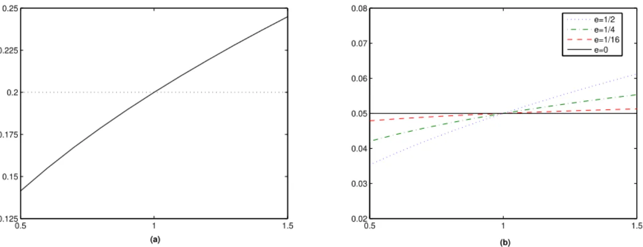
0.5 1 1.5 0.125
0.15 0.175 0.2 0.225 0.25
(a)
0.5 1 1.5
0.02 0.03 0.04 0.05 0.06 0.07 0.08
e=1/2 e=1/4 e=1/16 e=0
(b)
Figure 2: (a) : γ(I) for different levels of m(I) vs naive constant volatility ¯γ = 0.2. (b):λ(I), for different levels ofm(I) and differentǫ= 0,1/16,1/4,1/2, ¯λ= 0.05.
We note that we can interpret the intensity function as a function of the index level or, if we prefer, as a function of the index volatility. One can argue that the intensity should not be affected by index level, but instead by its volatility since it is the volatility that represents the “risk”. The above definition includes the two possibilities.
∂λ ∂I = ¯|{z}λǫ
>0
(m(I))ǫ−1
| {z }
>0
∂m(I)
∂I
| {z }
<0
<0 , ∂λ ∂γ =
¯
λ
¯
γ
|{z}
>0
[m(I)]ǫ−12
| {z }
>0
>0.
Figure 2 show the functionsλ(I) andγ(I) for different values ofm(I).
4.3
The loss quota
q
Finally, we need to decide on the loss quota distribution. As before, we make use of themratio for defining the of loss process distribution on the market indexI. We choose the Beta class of distributions. 9 We take
q∼Beta(2m(I),2) i.e. a= 2m(I) and b= 2, (12) which is consistent with the desired properties referred in Assumption 3.3. Thus,
˜
K(q, I) = 1
B(2m(I),2) Z q
0
x2m(I)−1(1−x)dx .
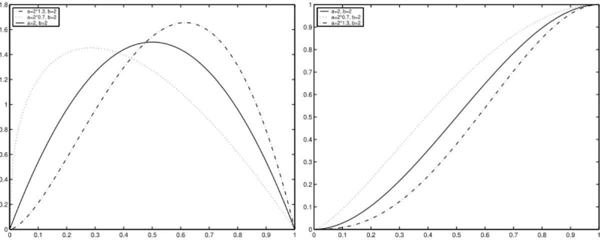
Figure 3 shows the loss quota density and its cumulative distribution function for three different values of m: m = 0.7 representing a bull market, m= 1 for the case where the market is at its long run level, and m= 1.3 representing a bear market. From the properties of the Beta
9Recall the beta density function is given byf(x) = 1 B(a,b)x
a−1(1−x)b−11
(0,1)(x) wherea >0,b >0 and B(a, b) =
Z1
0
xa−1(1−x)b−1ds (beta function). Useful properties of the beta distribution are
E[X] = a
a+b =µ , VarX=
ab
(a+b+ 1)(a+b)2 , E[(X−µ) r
] =B(r+a, b)
0 0.1 0.2 0.3 0.4 0.5 0.6 0.7 0.8 0.9 1 0
0.2 0.4 0.6 0.8 1 1.2 1.4 1.6 1.8
a=2*1.3, b=2 a=2*0.7, b=2 a=2, b=2
0 0.1 0.2 0.3 0.4 0.5 0.6 0.7 0.8 0.9 1 0
0.1 0.2 0.3 0.4 0.5 0.6 0.7 0.8 0.9 1
a=2, b=2 a=2*0.7, b=2 a=2*1.3, b=2
Figure 3: Density and Cumulative distribution functions of loss quota form= 1.3,m= 1,m= 0.7
distribution we get that the expected loss is given by
qe(I) =E[q(I)] = m(I)
1 +m(I), and
∂qe(I)
∂I =
∂m(I)
∂I
(1 +m(I))2 <0. (13)
Furthermore
• if default occurs exactly at the long-run level the loss expected quota is exactly 1/2;
• if default occurs when the index level is “high” (m < 1) one expects to recover more, expected loss quota decreases;
• if default occurs when the index level is “low” (m > 1) one expects to recover less, expected loss quota increases.
0 0.5 1 1.5 2
0 0.1 0.2 0.3 0.4 0.5 0.6 0.7 0.8 0.9 1
0 0.01 0.02 0.03 0.04 0.05 0.06 0.07 0.08 0
0.1 0.2 0.3 0.4 0.5 0.6 0.7 0.8 0.9 1
Intensity
Recovery corr =−0,6638
Figure 4: Left: Loss quota possible realizations and expected value for different values ofm. Dotted line is the naiveq= 1
2. Right: Scatter plot of intensity versus a recovery realization for different values
ofm.
4.4
Simulation Results
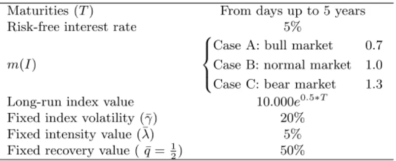
In simulations we use the Monte Carlo method where the step size is equivalent to one trading day (we do 250 steps per year) and all simulations concern 5,000 paths. The same noise matrix is used for all scenarios and cases so that the values obtained can actually be compared (discretization errors would be in the same direction for all scenarios). The spreads with zero maturity correspond to the short spread; all other maturities correspond to the forward spread. Table 1 tells us the reference parameters, while Table 2 characterizes all possible scenarios.
REFERENCE PARAMETERS
Maturities (T) From days up to 5 years
Risk-free interest rate 5%
m(I)
Case A: bull market 0.7
Case B: normal market 1.0
Case C: bear market 1.3
Long-run index value 10.000e0.5∗T
Fixed index volatility (¯γ) 20%
Fixed intensity value (¯λ) 5%
Fixed recovery value ( ¯q=1
2) 50%
Table 1: Reference values for the parameters in the model.
DIFFERENT SCENARIOS
Scenario Index Volatility Intensity Recovery
(1) F F F
(2) S F F
(3) F F S
(4) S F S
(5) F S F
(6) S S F
(7) F S S
(8) S S S
Table 2: Basic reference scenarios for simulations. F= Fixed, S= Stochastic.
4.4.1 Impacts on the term structure of forward credit spreads
( a )
0 .0 % 1 .0 % 2 .0 % 3 .0 % 4 .0 % 5 .0 % 6 .0 % 7 .0 %
0 0 .5 1 1 .5 2 2 .5 3 3 .5 4 4 .5 5 ( 1 ) ( 2 )
( 4 ) ( 3 ) ( 5 ) ( 6 ) ( 7 ) ( 8 )
( b )
0 .0 % 0 .5 % 1 .0 % 1 .5 % 2 .0 % 2 .5 % 3 .0 % 3 .5 % 4 .0 % 4 .5 %
0 0 .5 1 1 .5 2 2 .5 3 3 .5 4 4 .5 5
( 8 )
( 7 )
( 1 ) ( 2 ) ( 5 )
( 3 ) ( 6 )
( 4 )
( c )
0 .0 % 0 .5 % 1 .0 % 1 .5 % 2 .0 % 2 .5 % 3 .0 % 3 .5 % 4 .0 % 4 .5 %
0 0 .5 1 1 .5 2 2 .5 3 3 .5 4 4 .5 5 ( 8 ) ( 7 ) ( 6 ) ( 5 )
( 4 )( 3 ) ( 1 ) ( 2 )
C a se C : B e a r M a rke t
2.0% 2.5% 3.0% 3.5% 4.0% 4.5% 5.0%
0 2.5 5 7.5 10 12.5 15 17.5 20
(1)(2) (4) (3) (5) (6) (7) (8) C a se A : B ull M a rke t
1.8% 2.0% 2.2% 2.4% 2.6% 2.8% 3.0% 3.2%
0 2.5 5 7.5 10 12.5 15 17.5 20
(8) (7)
(6) (5)
(3)
(4) (1)(2)
C a se B : N orma l M a rke t
2.0% 2.2% 2.4% 2.6% 2.8% 3.0% 3.2% 3.4% 3.6% 3.8% 4.0%
0 2.5 5 7.5 10 12.5 15 17.5 20
(1)(2) (3) (4) (5) (6) (7) (8)
the dependence of both PD and LGD and the negative relation the index level and volatility (scenario (8)), the TS seems to converge faster to its long-run level. In fact, for maturities higher than 15 years the TS of this scenario is relatively flat. Thus, the forward credit spreads are most sensitive to the influence of the market index at the relatively shorter maturities, and around the 15 years maturity, the credit spreads become relatively flatter and less sensitive to the market index, moving in fact closer to each other.
4.4.2 Impacts on pricing and survival probabilities
Tables 3 and 4 presents forward spreads and defaultable bonds prices (non-zero recovery) for several maturities, low and high maturities respectively. The first point that should be high-lighted is that even for low maturities there is a difference in the prices produces by naive scenario (scenarios (1) and (2)), scenarios where either the PD or LGD is dependent on the index level (scenarios (3),(4),(5),(6)), and scenarios where we consider the combined effect. For the bull and bear markets the pricing difference in clear already atT = 0.1. At 5 year ma-turities the under pricing of the naive model can be of up to 5% in a bull market, and up to 10% in a bear market. When we consider longer horizons, from 5 to 15 years, in the stochastic volatility scenario, the survival probability decreases by almost 40% for the bull market and up to 50% for the bear market. In our opinion, this is a realistic feature of the model since at the longer horizons when the market is in recession and firms are known to be sensitive to the fluctuations of the market, the probability of default is quite high. Moreover, it is interesting to note that in a bull market, although a stochastic volatility scenario yields higher survival probabilities at all the maturities, the difference in survival probabilities is much smaller at the higher maturities. In a bear market, on the other hand, survival probabilities are lower for the stochastic volatility case, and the difference in survival probabilities between the stochastic volatility and naive scenarios is more pronounced. In contrast to the bull market, the difference increases by approximately 5% when the investment horizon is extended from 5 to 15 years.
4.4.3 How to account for different ratings
We now take a closer look at the parameter ǫwhich we recall (Assumption 3.2) is a measure of the sensitivity of a firms PD to the market situation. The intuition comes from the fact the PD of firms with high credit worthiness should depend very little (or not depend at all) on the market oscillation while less credit worthy firms are more sensitive to business cycles. In this sense, differentǫ parameters could represent the term structure of firms with different credit ratings. In the following we consider three different values for epsilon: high ǫ = 1/2, medium ǫ = 1/4 and low ǫ= 1/16.10 Figure 7 and Tables 5 show the simulation results for
the different ǫvalues under normal market conditions. The key feature is that the TS of less sensitive (higher ratings) firms have a smaller slope. This is particularly obvious for scenarios (7) and (8) when the index influences both PD and LGD, and less obvious when it affects only one of them. Thus, from a practical point of view, it is more important to take into account the correlation with the market index, especially when considering a portfolio of securities with low credit ratings. The effect will be even more pronounced when we have stochastic index volatility.
T (1)(2) (3) (4) (5) (6) (7) (8)
0 2.500% 2.174% 2.174% 2.192% 2.192% 1.906% 1.906%
0.1 2.500% 2.177% 2.176% 2.196% 2.195% 1.914% 1.912% 0.5 2.500% 2.188% 2.185% 2.209% 2.206% 1.945% 1.937%
1 2.500% 2.201% 2.196% 2.226% 2.220% 1.983% 1.968%
1.5 2.500% 2.215% 2.208% 2.245% 2.236% 2.025% 2.006%
2 2.500% 2.228% 2.219% 2.262% 2.251% 2.063% 2.040%
3 2.500% 2.253% 2.241% 2.296% 2.284% 2.140% 2.112%
5 2.500% 2.299% 2.275% 2.355% 2.334% 2.264% 2.217%
T (1)(2) (3) (4) (5) (6) (7) (8) 0 2.5000% 2.5000% 2.5000% 2.5000% 2.5000% 2.5000% 2.5000% 0.1 2.5000% 2.5025% 2.5025% 2.5038% 2.5038% 2.5088% 2.5088% 0.5 2.5000% 2.5124% 2.5126% 2.5189% 2.5193% 2.5440% 2.5450% 1 2.5000% 2.5246% 2.5247% 2.5376% 2.5386% 2.5869% 2.5894% 1.5 2.5000% 2.5362% 2.5378% 2.5573% 2.5612% 2.6327% 2.6416% 2 2.5000% 2.5479% 2.5492% 2.5755% 2.5816% 2.6736% 2.6875% 3 2.5000% 2.5700% 2.5736% 2.6142% 2.6300% 2.7606% 2.7953% 5 2.5000% 2.6121% 2.6145% 2.6836% 2.7178% 2.9082% 2.9769%
T (1)(2) (3) (4) (5) (6) (7) (8) 0 2.5000% 2.9413% 2.9411% 2.9881% 2.9880% 3.5157% 3.5155% 0.1 2.5000% 2.9433% 2.9439% 2.9925% 2.9941% 3.5258% 3.5296% 0.5 2.5000% 2.9512% 2.9551% 3.0103% 3.0199% 3.5672% 3.5897% 1 2.5000% 2.9608% 2.9687% 3.0324% 3.0533% 3.6182% 3.6666% 1.5 2.5000% 2.9704% 2.9822% 3.0544% 3.0882% 3.6686% 3.7458% 2 2.5000% 2.9803% 2.9940% 3.0742% 3.1167% 3.7121% 3.8084% 3 2.5000% 2.9982% 3.0201% 3.1189% 3.1985% 3.8114% 3.9857% 5 2.5000% 3.0303% 3.0688% 3.2088% 3.4289% 4.0014% 4.4276%
Case C : Bear Market Case B : Normal Market
(a) SPREADS
Case A : Bull Market
T (1)(2) (3) (4) (5) (6) (7) (8) 0.1 0.9925 0.9928 0.9928 0.9928 0.9928 0.9930 0.9930 0.5 0.9631 0.9647 0.9647 0.9646 0.9646 0.9659 0.9659
1 0.9277 0.9306 0.9306 0.9304 0.9304 0.9328 0.9329
1.5 0.8935 0.8976 0.8977 0.8973 0.8974 0.9007 0.9009
2 0.8606 0.8658 0.8659 0.8654 0.8655 0.8696 0.8698
3 0.7985 0.8053 0.8055 0.8046 0.8048 0.8100 0.8104
5 0.6872 0.6963 0.6966 0.6949 0.6953 0.7013 0.7021
T (1)(2) (3) (4) (5) (6) (7) (8) 0.1 0.9924 0.9924 0.9924 0.9924 0.9924 0.9924 0.9924 0.5 0.9631 0.9631 0.9631 0.9631 0.9631 0.9630 0.9630
1 0.9277 0.9275 0.9275 0.9275 0.9275 0.9272 0.9272
1.5 0.8935 0.8933 0.8933 0.8931 0.8931 0.8926 0.8926
2 0.8606 0.8602 0.8602 0.8600 0.8599 0.8591 0.8590
3 0.7984 0.7976 0.7975 0.7971 0.7970 0.7953 0.7950
5 0.6872 0.6852 0.6852 0.6840 0.6836 0.6800 0.6792
T (1)(2) (3) (4) (5) (6) (7) (8) 0.1 0.9924 0.9920 0.9920 0.9919 0.9919 0.9914 0.9914 0.5 0.9631 0.9609 0.9609 0.9607 0.9606 0.9581 0.9580
1 0.9276 0.9234 0.9234 0.9229 0.9228 0.9178 0.9176
1.5 0.8935 0.8874 0.8873 0.8865 0.8863 0.8789 0.8785
2 0.8606 0.8527 0.8526 0.8515 0.8511 0.8416 0.8407
3 0.7984 0.7872 0.7870 0.7853 0.7844 0.7710 0.7692
5 0.6872 0.6706 0.6700 0.6670 0.6644 0.6452 0.6400
(b) ZERO-COUPON DEFAULTABLE BONDS W/ RECOVERY
Case A : Bull Market
Case B : Normal Market
Case C : Bear Market
T
abl
e
3:
(a)
Cr
edit
Spr
eads
and
(b)
Pr
ice
of
default
able
b
ond
wit
h
reco
v
er
y,
for
sev
er
al
shor
t
mat
ur
it
ies
T (1)(2) (3) (4) (5) (6) (7) (8)
5 2.500% 2.299% 2.275% 2.355% 2.334% 2.264% 2.217%
6 2.5000% 2.3222% 2.2990% 2.3940% 2.3838% 2.3494% 2.3231% 7 2.5000% 2.3432% 2.3166% 2.4248% 2.4137% 2.4120% 2.3825% 8 2.5000% 2.3633% 2.3338% 2.4573% 2.4603% 2.4769% 2.4691% 10 2.5000% 2.4016% 2.3632% 2.5188% 2.5416% 2.5916% 2.6039% 12 2.5000% 2.4371% 2.3910% 2.5774% 2.6189% 2.6953% 2.7190% 15 2.5000% 2.4824% 2.4302% 2.6739% 2.7691% 2.8554% 2.8981% 20 2.5000% 2.5542% 2.4668% 2.7863% 2.8439% 2.9922% 2.8864%
T (1)(2) (3) (4) (5) (6) (7) (8) 5 2.5000% 2.6121% 2.6145% 2.6836% 2.7178% 2.9082% 2.9769% 6 2.5000% 2.6310% 2.6404% 2.7281% 2.8012% 3.0045% 3.1441% 7 2.5000% 2.6495% 2.6595% 2.7625% 2.8530% 3.0731% 3.2376% 8 2.5000% 2.6671% 2.6768% 2.7988% 2.9226% 3.1432% 3.3545% 10 2.5000% 2.7011% 2.7054% 2.8669% 3.0235% 3.2643% 3.4930% 12 2.5000% 2.7326% 2.7315% 2.9314% 3.1352% 3.3706% 3.6233% 15 2.5000% 2.7696% 2.7640% 3.0359% 3.2997% 3.5253% 3.7635% 20 2.5000% 2.8352% 2.7992% 3.1547% 3.3834% 3.6428% 3.7094%
T (1)(2) (3) (4) (5) (6) (7) (8) 5 2.5000% 3.0303% 3.0688% 3.2088% 3.4289% 4.0014% 4.4276% 6 2.5000% 3.0434% 3.0890% 3.2580% 3.5343% 4.0992% 4.6167% 7 2.5000% 3.0582% 3.1067% 3.2979% 3.6118% 4.1738% 4.7347% 8 2.5000% 3.0720% 3.1210% 3.3398% 3.7093% 4.2486% 4.8668% 10 2.5000% 3.0994% 3.1449% 3.4174% 3.8324% 4.3721% 4.9761% 12 2.5000% 3.1247% 3.1631% 3.4899% 3.9246% 4.4752% 5.0054% 15 2.5000% 3.1505% 3.1813% 3.6048% 4.1097% 4.6074% 5.0888% 20 2.5000% 3.2070% 3.2096% 3.7295% 4.2577% 4.6777% 4.9864%
Case C : Bear Market Case B : Normal Market
(a) SPREADS
Case A : Bull Market
T (1)(2) (3) (4) (5) (6) (7) (8)
5 0.6872 0.6963 0.6966 0.6949 0.6953 0.7013 0.7021
6 0.6374 0.6470 0.6475 0.6454 0.6459 0.6518 0.6529
7 0.5913 0.6012 0.6019 0.5993 0.5998 0.6054 0.6066
8 0.5486 0.5586 0.5594 0.5563 0.5568 0.5619 0.5632
10 0.4722 0.4819 0.4829 0.4789 0.4792 0.4832 0.4843
12 0.4064 0.4155 0.4167 0.4118 0.4118 0.4147 0.4155
15 0.3245 0.3321 0.3336 0.3275 0.3268 0.3283 0.3285
20 0.2231 0.2281 0.2299 0.2226 0.2215 0.2209 0.2217
T (1)(2) (3) (4) (5) (6) (7) (8)
5 0.6872 0.6852 0.6852 0.6840 0.6836 0.6800 0.6792
6 0.6373 0.6347 0.6346 0.6330 0.6322 0.6276 0.6261
7 0.5913 0.5880 0.5878 0.5858 0.5846 0.5791 0.5768
8 0.5485 0.5446 0.5444 0.5419 0.5402 0.5340 0.5308
10 0.4721 0.4670 0.4668 0.4633 0.4605 0.4531 0.4483
12 0.4064 0.4003 0.4000 0.3956 0.3917 0.3836 0.3776
15 0.3245 0.3172 0.3170 0.3113 0.3060 0.2976 0.2907
20 0.2230 0.2147 0.2148 0.2077 0.2020 0.1938 0.1882
T (1)(2) (3) (4) (5) (6) (7) (8)
5 0.6872 0.6706 0.6700 0.6670 0.6644 0.6452 0.6400
6 0.6372 0.6185 0.6176 0.6138 0.6098 0.5888 0.5811
7 0.5911 0.5707 0.5696 0.5650 0.5597 0.5373 0.5274
8 0.5484 0.5264 0.5252 0.5199 0.5132 0.4900 0.4781
10 0.4720 0.4478 0.4463 0.4397 0.4305 0.4067 0.3918
12 0.4063 0.3808 0.3792 0.3713 0.3604 0.3368 0.3207
15 0.3244 0.2983 0.2967 0.2872 0.2748 0.2529 0.2369
20 0.2230 0.1982 0.1969 0.1862 0.1741 0.1561 0.1438
Case C : Bear Market
(b) ZERO-COUPON DEFAULTABLE BONDS W/ RECOVERY
Case A : Bull Market
Case B : Normal Market
T
abl
e
4:
(a)
Cr
edit
Spr
eads
and
(b)
Pr
ice
of
default
able
b
ond
wit
h
reco
v
er
y,
for
sev
er
al
long
mat
ur
it
ies
H ig h S e n s it ivit y
2 .2 % 2 .3 % 2 .4 % 2 .5 % 2 .6 % 2 .7 % 2 .8 % 2 .9 % 3 .0 % 3 .1 %
0 0.5 1 1.5 2 2.5 3 3.5 4 4.5 5 ( 8)
( 7)
(6 ) ( 5)
( 3) ( 4)
( 1) ( 2)
M e d iu m S e n s it ivit y
2.2% 2.3% 2.4% 2.5% 2.6% 2.7% 2.8% 2.9% 3.0% 3.1%
0 0.5 1 1.5 2 2.5 3 3.5 4 4.5 5 ( 1) ( 2)
( 5) ( 6) ( 8)
( 7)
( 3) ( 4)
L o w s e n s it ivit y
2.2% 2.3% 2.4% 2.5% 2.6% 2.7% 2.8% 2.9% 3.0% 3.1%
0 0.5 1 1.5 2 2.5 3 3.5 4 4.5 5 ( 1) ( 2)
( 8) ( 7) ( 4) ( 3)
( 5)( 6)
T (1)(2) (3) (4) (5) (6) (7) (8) 0 2.5000% 2.5000% 2.5000% 2.5000% 2.5000% 2.5000% 2.5000% 0.1 2.5000% 2.5025% 2.5025% 2.5038% 2.5038% 2.5088% 2.5088% 0.5 2.5000% 2.5124% 2.5126% 2.5189% 2.5193% 2.5440% 2.5450% 1 2.5000% 2.5246% 2.5247% 2.5376% 2.5386% 2.5869% 2.5894% 1.5 2.5000% 2.5362% 2.5378% 2.5573% 2.5612% 2.6327% 2.6416% 2 2.5000% 2.5479% 2.5492% 2.5755% 2.5816% 2.6736% 2.6875% 3 2.5000% 2.5700% 2.5736% 2.6142% 2.6300% 2.7606% 2.7953% 5 2.5000% 2.6121% 2.6145% 2.6836% 2.7178% 2.9082% 2.9769%
T (1)(2) (3) (4) (5) (6) (7) (8) 0 2.5000% 2.5000% 2.5000% 2.5000% 2.5000% 2.5000% 2.5000% 0.1 2.5000% 2.5025% 2.5025% 2.5016% 2.5016% 2.5054% 2.5053% 0.5 2.5000% 2.5124% 2.5126% 2.5079% 2.5080% 2.5266% 2.5271% 1 2.5000% 2.5246% 2.5247% 2.5157% 2.5160% 2.5525% 2.5535% 1.5 2.5000% 2.5362% 2.5378% 2.5236% 2.5252% 2.5792% 2.5837% 2 2.5000% 2.5479% 2.5492% 2.5313% 2.5335% 2.6038% 2.6099% 3 2.5000% 2.5700% 2.5736% 2.5471% 2.5527% 2.6544% 2.6697% 5 2.5000% 2.6121% 2.6145% 2.5768% 2.5879% 2.7433% 2.7701%
T (1)(2) (3) (4) (5) (6) (7) (8) 0 2.5000% 2.5000% 2.5000% 2.5000% 2.5000% 2.5000% 2.5000% 0.1 2.5000% 2.5025% 2.5025% 2.5003% 2.5003% 2.5032% 2.5032% 0.5 2.5000% 2.5124% 2.5126% 2.5017% 2.5017% 2.5156% 2.5159% 1 2.5000% 2.5246% 2.5247% 2.5033% 2.5034% 2.5310% 2.5313% 1.5 2.5000% 2.5362% 2.5378% 2.5050% 2.5053% 2.5460% 2.5482% 2 2.5000% 2.5479% 2.5492% 2.5067% 2.5070% 2.5606% 2.5629% 3 2.5000% 2.5700% 2.5736% 2.5100% 2.5110% 2.5891% 2.5951% 5 2.5000% 2.6121% 2.6145% 2.5165% 2.5184% 2.6419% 2.6491%
Low (a) SPREADS
High
Medium
T (1)(2) (3) (4) (5) (6) (7) (8) 0.1 0.9924 0.9924 0.9924 0.9924 0.9924 0.9924 0.9924 0.5 0.9631 0.9631 0.9631 0.9631 0.9631 0.9630 0.9630
1 0.9277 0.9275 0.9275 0.9275 0.9275 0.9272 0.9272
1.5 0.8935 0.8933 0.8933 0.8931 0.8931 0.8926 0.8926
2 0.8606 0.8602 0.8602 0.8600 0.8599 0.8591 0.8590
3 0.7984 0.7976 0.7975 0.7971 0.7970 0.7953 0.7950
5 0.6872 0.6852 0.6852 0.6840 0.6836 0.6800 0.6792
T (1)(2) (3) (4) (5) (6) (7) (8) 0.1 0.9924 0.9924 0.9924 0.9924 0.9924 0.9924 0.9924 0.5 0.9631 0.9631 0.9631 0.9631 0.9631 0.9630 0.9630
1 0.9277 0.9275 0.9275 0.9276 0.9276 0.9274 0.9274
1.5 0.8935 0.8933 0.8933 0.8934 0.8933 0.8930 0.8930
2 0.8606 0.8602 0.8602 0.8604 0.8603 0.8597 0.8597
3 0.7984 0.7976 0.7975 0.7979 0.7978 0.7966 0.7964
5 0.6872 0.6852 0.6852 0.6859 0.6858 0.6829 0.6826
T (1)(2) (3) (4) (5) (6) (7) (8) 0.1 0.9924 0.9924 0.9924 0.9924 0.9924 0.9924 0.9924 0.5 0.9631 0.9631 0.9631 0.9631 0.9631 0.9631 0.9631
1 0.9277 0.9275 0.9275 0.9276 0.9276 0.9275 0.9275
1.5 0.8935 0.8933 0.8933 0.8935 0.8935 0.8932 0.8932
2 0.8606 0.8602 0.8602 0.8606 0.8606 0.8601 0.8601
3 0.7984 0.7976 0.7975 0.7983 0.7983 0.7974 0.7973
5 0.6872 0.6852 0.6852 0.6869 0.6869 0.6847 0.6846
(b) ZERO-COUPON DEFAULTABLE BONDS W/ RECOVERY
15% 17% 19% 21% 23% 25% 27% 29% 31% 33% 35%
0 0.5 1 1.5 2 2.5 3 3.5 4 4.5 5
(a)
(b)
(c)
Figure 8: Volatility paths corresponding to the spot spread paths.
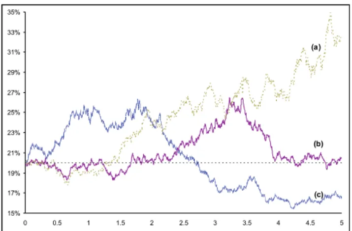
4.4.4 Using implied ATM volatilities as credit spread trackers
An interesting side effect of our concrete model is that, when we take the index volatility to be stochastic and negatively related to the index level, the short spread dynamics can be tracked quite well by observing the index volatility. See Figure 8 with three possible volatility paths and compare with the short spread evolution in Figure 5. An interesting conjecture arises: since the (spot) volatility seems to be a good tracker of the short spread, then implied volatilities of options with longer maturities may be good trackers of the forward spread TS. This is all due to the negative correlation between the index level and its volatility. Still, it provides a fundamental reason for using implied volatilities of options on indices as predictors of forward credit spread term structures, which seems to be common practice among traders (who use ATM volatility term structures as predictors). Collin-Dufresne, Goldstein, and Martin (2001) also investigated the determinants of credit spread and showed that credit spreads are mostly driven by a single common factor and that implied volatilities of index options contain important information for credit spreads11.
4.5
Calibration of the model to market data
Lack of the closed form solutions complicates the calibration procedure. In order to calibrate our concrete model to the observed credit spreads, we specify its intensity and expected loss quota as a perturbation of the naive model. We thenlinearizethe observed bond prices in the perturbation parameter around the value k= 0. Concretely, we specify the intensity and the loss quota as follows
λ(m(I)) =λ{1 +km(I)}ǫ qe(m(I)) = a(1 +km(I))
a(1 +km(I)) +b, (14)
11Recent papers (see e.g. Cremers, Dreissen, and Weinbaum (2004)) start using measures of volatility and
Estimation results
Default intensityλ 0.0105 (0.0039)
SensitivityǫAaa 0.0737 (1.0555)
SensitivityǫBbb 0.9001 (3.7663)
Volatility of indexγ 0.35 (0.0017)
Beta-distribution param. a 1.8587 (0.0984) Beta-distribution param. b 11.5947 (0.2286)
Perturbation param. k 1.6738 (0.1594)
Table 6: Least-square estimates of the model parameters (standard deviations in brackets).
where we assume that the Beta distribution, for the loss quota, has parametersa(1 +km(I)) andb.
We observe that if k = 0 the model reduces to the naive model (constant intensity λ and constant expected loss quotaqe= a
a+b).
Our data consists of daily data from august 2004 to march 2007, on benchmark yields of Moody’s Aaa and Bbb rated long term US corporate bonds. We use long term US government yields as a proxy to the risk-free short rate the S&P 500 as our market index. Since the data comes in
yields we note that the yield spread between the defaultable and non-defaultable bonds can be computed as follows
¯
y(t, T)−y(t, T) =− 1
T−t
Z T
t
s(t, u, k)du, (15)
wheres(t, T, k) can be found as in (7).
In order to be able to calibrate our model to the observed credit yield spreads we linearize
s(t, T, k) around the value k = 0, that is we find the linear perturbation of the benchmark model in the parameterk.
¯
y(t, T)−y(t, T) =− 1
T−t
Z T
t
s(t, u,0) +∂s(t, u,0)
∂k k
du
= λa
a+b+ λa
(a+b)2
(1 +ǫ)(a+b)−a T−t
1
γ2
2 −r
e(T−t)(γ
2 2−r)−1
¯
I It
∆k (16)
We use our model to create model-consistent time series of yields of corporate bond and find the set of parameters which minimizes the difference (in the least square sense) to the observed term structure. We present the estimation results in Table 6. Figure 9 shows theestimatedloss quota density function for three different values ofm(I): m= 0.7 representing a bull market,
m= 1 for the case where the market is at its long run level, andm= 1.3 representing a bear market.
5
Conclusions and future research
0 0.2 0.4 0.6 0.8 1 0
0.5 1 1.5 2 2.5 3 3.5 4
normal market bull market beer market
Figure 9: Estimated beta-distribution for loss quotas
qualitative properties of both the intensity and the loss quota distribution. Finally, we discuss (in) existence of tractable models that would that into account all the required properties.
We then use a concrete (simple) instance of our class of model and use simulations to compute survival probabilities, defaultable bond prices, and forward spread term structures and show that it is possible to account for many empirically observed features, such as:
• the difference between short spreads in bull versus bear markets can be up to three times more than the difference produced by models that consider the market influence in the PD or LGD only;
• the convergence to long-run levels is faster, originating flat TS for maturities higher than 15 years;
• market volatility tracks the short credit spread dynamics quite well, suggesting that the TS of ATM implied volatilities of index options may do the same for forward credit spreads.
Given the simplicity of the proposed concrete model we found this extremely encouraging. We also show how we can calibrate models with no closed-form solutions to market data and use US market data to calibrate our own concrete model.
A
Appendix
Proof of Theorem 2.5:
Proof. We fixΩ,F,P,(Ft)0≤t≤T
and a Marked Point Process ˆµwith the compensator
ˆ
ν(dt, dq) =mt(dq)dt
and, as before,GW
t =GW ∨ F µ
t. Since Mt(x, dq) is absolutely continuous w.r.t mt(dq) onE,
then according to the Radon-Nikodym Theorem for everyt there exists aE × GW-measurable
nonnegative function ϕt(q, x),ϕ:E×R+→R+, such that
M(t, Ax) = Z
A
ϕ(t, q, x)m(t, dq), for all A∈ E
or
M(t, dq, x) =ϕ(t, q, x)m(t, dq).
We define the processLt as
(
dLt = Lt− R
E{ϕ(t, q, Xt)−1} {µˆ(dt, dq)−mt(dq)dt}
L0 = 1.
We notice thatϕ(t, q, Xt)∈ GW0 . Define the new measure on GtW, 0≤t ≤T as dQ=LtdP.
According to the Girsanov transformation theQ-compensator of the new process is exactly
ν(dt, dq) = ˆν(dt, dq)(1 +ϕt(q, Xt)−1) =ϕt(q, Xt)mt(dq)dt=Mt(dq, Xt)dt.
First, we would like to show that theQ-distribution ofν is the same as theP-distribution. We note thatGW
0 =GW and that
dQ
dP GW
0 =L0= 1, thus,P=QonGW
0 . Second, we would like to show that
P µ((s, t]×B) =kGsW
= (ν((s, t]×B))
k
k! e
−ν((s,t]×B), a.s., B∈E. (17)
We prove (17) using characteristic functions. Define the stochastic process
Yt=
Z t
0
Z
E
qµˆ(ds, dq).
Changing the measure we obtain that
EQeiuYtGW
0
=EPLteiuYt
GW
0
.
DefineZt =LteiuYt, then the dynamics ofZt is
dZt = Lt
Z
E
n
eiu(Yt−+q)−eiuYt−
o
µ(dt, dq)
+Lt−eiuYt Z
E
(ϕ(t, q, Xt)−1){µˆ(dt, dq)−mt(dq)dt}
+ Z
E
Lt−(ϕ(t, q, Xt)−1)
n
eiu(Yt−+q)−eiuYt−
o ˆ
µ(dt, dq)
= Z
E
Zt−ϕ(t, q, Xt)mt(dq)(eiuq−1)dt+
Z
E
Zt−(eiuq−1)ϕ(t, q, Xt)˜µ(dt, dq)
+ Z
E
where ˜µ(dt, dq) = ˆµ(dt, dq)−mt(dq). We notice also thatZ0= 1, then
Zt = 1 +
Z t
0
Z
E
Zs−ϕ(s, q, Xs)mt(dq)(eiuq−1)ds+
Z t
0
. . .µ˜(ds, dq)
= 1 +
Z t
0
Z
E
Zs−(eiuq−1)Ms(dq, Xs)ds+
Z t
0
. . .µ˜(ds, dq).
Denoteξt=EPZt| G0W
, then
ξt= 1 +
Z t
0
Z
E
ξs(eiuq−1)Ms(dq, Xs)ds.
thus sinceξt does not depend onqandMs(dq, Xs) isG0W-measurable
ξt =e
Rt
0
R
E(e iuq−1)M
s(dq,Xs)ds.
Note thatν(dt, dq, Xt) =Mt(dq, Xt)dtisGW measurable. The final result follows from the fact
that the characteristic function of the process
¯
Yt=
Z t
0
Z
E
qµ¯(ds, dq)
where ¯µis a Marked Poisson Process with compensator ¯ν(t, dq) is given by
EheiuY¯t
i = exp
Z t
0
Z
E
(eiuq−1)¯ν(s, dq)
.
Lemma A.1. Consider a T-defaultable claimX. For the purpose of computing expectations,
and in particular its price at timet≤T
EQt heRtTrsdsV(T)X
i
,
it is equivalent to use the following two dynamics for the remaining value process
dV(t)
V(t−) =− Z 1
0
qµ(dt, dq), V(t) =v (18)
and
dV(t)
V(t−) =−q
e(t−, X
t−)dNt, V(t) =v (19)
where µ is a DSMPP with compensator ν(t, Xt) =λ(t, Xt)K(t, dq, Xt)dt, N is a Cox process
with intensityλ(t, Xt), and we define
qe(t, X t) =
Z 1
0
Proof. Using theV dynamics in (18) we get,
EQhe−RT
t rsdsV(T)X
Ft
i =
=V(t)EQhe−RtTrsdsX
Ft
i
| {z }
π(t,X)
−EQ "
e−RtTrsds
Z T
t
Z 1
0
qVs−µ(dq, ds)X Ft #
=V(t)π(t,X)−EQ "
EQ "
e−RtTrsds
Z T
t
Z 1
0
qVs−µ(dq, ds)X GW t # Ft #
=V(t)π(t,X)−EQ "
e−RtTrsds
Z T
t
Vs−
Z 1
0
qK(s, dq, Xs)
λ(s, Xs)dsX
Ft #
=V(t)π(t,X)−EQ "
e−RtTrsds
Z T
t
Vs−qe(s, Xs)λ(s, Xs)dsX
Ft #
Using theV dynamics in (19) we get,
EQhe−RtTrsdsV(T)X
Ft
i =
=V(t)EQ h
e−RtTrsdsX
Ft
i
| {z }
π(t,X)
−EQ "
e−RtTrsds
Z T
t
Vs−qe(s, Xs)dN(s)X
Ft #
=V(t)π(t,X)−EQ "
EQ "
e−RtTrsds
Z T
t
Vs−qe(s, Xs)dN(s)X
GtW
# Ft #
=V(t)π(t,X)−EQ "
e−RtTrsdsEQ
" Z T
t
Vs−qe(s, Xs)dN(s)X
GWt
# Ft #
=V(t)π(t,X)−EQ "
e−RtTrsds
Z T
t
Vs−qe(s, Xs)λ(s, Xs)dsX
Ft #
The results follow from comparing the final expressions on both cases.
Proof of Proposition 2.7:
Proof. The timet price of the defaultable zero-coupon bond with maturityT is equal to
¯
p(t, T) =EQhe−RT
t rsdsV(T)
Ft
i
, (20)
whereV(T) is the residual of the face value after multiple defaults up to time T. Making use of Lemma A.1, instead of VdV(t(−t)) =−R01qµ(dt, dq) with our DSMPPµ(these dynamics follow directly from (3)), we use
dV(t)
V(t−)=−q
e(t−, X t−)dNt
whereN is the Cox process with intensityλ(t, Xt). For every fixedt, defineZ(u) as follows
Z(u) =eRtuq e(s,X
We note that then the dynamics ofZ(u) take the form
dZ(u) =−Zu−qe(u−, Xu−){dNu−λ(u, Xu)du} , u≥t, t-fixed
andZ(u) is aQ-martingale conditional on the filtrationFW t . Thus,
EQZ(T)| FtW
=Z(t).
The price of a defaultable bond is then can be found as
¯
p(t, T) = EQhe−RtTrsdsV(T)
Ft
i
=EQhe−RtTrsdse−
RT
t q e(s,X
s)λ(s,Xs)dsZ(T)
Ft
i
= EQhEQhe−RtTrsdse−
RT
t q e(s,X
s)λ(s,Xs)dsZ(T)
GtW
i Ft
i
= EQhe−RtTrsdse−
RT
t q e(
s,Xs)λ(s,Xs)dsEQZ(T)| GW
t Ft
i
= EQhe−RtTrsdse−
RT
t q e(s,X
s)λ(s,Xs)dsZ(t)
Ft
i
= V(t)EQhe−RT t {r(s)+q
e(s,X
s)λ(s,Xs)}ds
Ft
i
.
Using the basic relations between defaultable bond prices and defaultable forward rates in (??) we can, thus, write
¯
f(t, T) =
EQt h{r(T) +λ(T, XT)qe(T, XT)}e−
RT
t {r(s)+λ(s,Xs)qe(s,Xs)}ds
i
EQt he−RT
t {r(s)+λ(s,Xs)qe(s,Xs)}ds
i . (21)
Finally using that ¯f(t, t) = ¯r(t) in the above expression we obtain
¯
r(t, rt, Xt) =r(t) +qe(t, Xt)λ(t, Xt).
The result follow froms(t) = ¯r(t)−r(t) ands(t, T) = ¯f(t, T)−f(t, T).
References
Allen, L. and A. Saunders (2003). A survey of cyclical effects in credit risk measurement models. BIS Working papers N.126.
Altman, E., B. Braddy, A. Resti, and A. Sironi (2005). The link between default and recovery rates: theory, empirical evidence and implications.Journal of Bussiness 78, 2203–2228. Altman, E. B., A. Resti, and A. Sironi (2004). Default recovery rates in credit risk modelling:
a review of the literature and empirical evidence. Economic Notes by Banca Monte dei Paschi di Siena SpA 33(2), 183–308.
Basel Committee (2003).The new Basel capital Accord. Basel Comittee on Banking Super-vision.
Chen, L., D. Filipovi´c, and H. V. Poor (2004). Quadratic term structure models for risk-free and defaultable rates.Mathematical Finance 14(4), 515–536.
Collin-Dufresne, P., R. S. Goldstein, and J. S. Martin (2001). Individual stock-option prices and credit spreads.Journal of Finance 56(6), 2177–2207.
D¨ullmann, K. and M. Trapp (2000). Systematic risk in recovery rates - an empirical analy-sis of us corporate credit expousures. Discussion Paper Serie 2: Banking and Financial Supervision.
Elton, E. and M. J. Gruber (2004). Factors affecting the valuation of corporate bonds.Journal of Business and Finance 28(11), 31–53.
Frye, J. (2000a). Collateral damage.Risk 13(4), 91–94.
Frye, J. (2000b). Depressing recoveries.Risk Magazine November, 108–111. Frye, J. (2003). A false sense of security.Risk 16(8), 63–67.
Gaspar, R. M. (2001).Sobre o efeito da correla¸c˜ao entre rendibilidade e volatilidade do activo subjacente na valoriza¸c˜ao de op¸c˜oes. Serie Moderna Finan¸ca n.25, Euronext.
Gaspar, R. M. and T. Schmidt (2007). Shot-noise quadratic term structure models.submitted. Giese, G. (2005). The impact of PD/LGD correlations on credit risk capital. Risk
Maga-zine 8(4), 79–84.
Gordy, M. (2000). A comparative anatomy of credit risk models. Journal of Banking and Finance 24, 119–149.
Hu, Y. and W. Perrandin (2002). The dependence of recovery rates and default. Birbeck College and Bank of England working paper.
Jiang, G. and P. Sluis (1995). Index option pricing models with stochastic volatility and stochastic interest rates.Review of Finance 3, 273–310.
JP Morgan (1997). Creditmetrics. Technical Document.
Last, G. and A. Brandt (1995). Probability and its applications-Marked point processes on the real line. Spring verlag.
Saunders, A. (1999).Credit Risk measurement. John Wiley & Sons.
Sch¨onbucher, P. (2001). Factors models: portfolio credit risk when defaults are correlated.
Journal of Risk Finance 3(1), 31–53.
Sch¨onbucher, P. (2003).Credit derivatives pricing models - models, pricing and implementa-tion. JWS.
Selcuk, F. (2005). Asymmetric stochastic volatility models in emerging stock markets.Applied
Financial Economics 15, 867–874.
Wilde, T. (2001). IRB approach explained.Risk 14(5), 87–90.