ECONOMIC PERFORMANCE AND GOVERNMENT SIZE

W O R K I N G PA P E R S E R I E S

N O 1 3 9 9 / N O V E M B E R 2 011

by António Afonso

and João Tovar Jalles

ECONOMIC

PERFORMANCE AND

1 We are grateful to comments from an ECB WPs anonymous referee and to Roberta De Stefani for research assistance. Part of the research was conducted while João Tovar Jalles was visiting the Fiscal Policies Division at the ECB whose hospitality was greatly appreciated. The opinions expressed herein are those of the authors and do not necessarily reflect those of the ECB or the Eurosystem. 2 ISEG/UTL – Technical University of Lisbon, Department of Economics; UECE – Research Unit on Complexity and Economics. UECE is supported

by FCT (Fundação para a Ciência e a Tecnologia, Portugal); e-mail: aafonso@iseg.utl.pt and European Central Bank, Directorate

This paper can be downloaded without charge from http://www.ecb.europa.eu or from the Social Science Research Network electronic library at http://ssrn.com/abstract_id=1950570.

NOTE: This Working Paper should not be reported as representing the views of the European Central Bank (ECB). The views expressed are those of the authors and do not necessarily reflect those of the ECB.

W O R K I N G P A P E R S E R I E S

N O 13 9 9 / N O V E M B E R 2 011

ECONOMIC PERFORMANCE

AND GOVERNMENT SIZE

by António Afonso

_{and João Tovar Jalles}

© European Central Bank, 2011

Address

Kaiserstrasse 29

60311 Frankfurt am Main, Germany

Postal address

Postfach 16 03 19

60066 Frankfurt am Main, Germany

Telephone

+49 69 1344 0

Internet

http://www.ecb.europa.eu

Fax

+49 69 1344 6000 All rights reserved.

Any reproduction, publication and reprint in the form of a different publication, whether printed or produced electronically, in whole or in part, is permitted only with the explicit written authorisation of the ECB or the authors.

Information on all of the papers published in the ECB Working Paper Series can be found on the ECB’s website, http://www. ecb.europa.eu/pub/scientific/wps/date/ html/index.en.html

Abstract 4 Non-technical summary 5

1 Introduction 6

2 Model and econometric specifi cation 8

3 Data 11

4 Methodology and results 14 4.1 Baseline results 14 4.2 Endogeneity issues and dynamic

panel estimation 15

4.3 Fiscal rules 19

4.4 Robustness checks 20

5 Conclusion 24

References 25

Appendices 29

Abstract

We construct a growth model with an explicit government role, where more government resources reduce the optimal level of private consumption and of output per worker. In the empirical analysis, for a panel of 108 countries from 1970-2008, we use different proxies for government size and institutional quality. Our results, consistent with the presented growth model, show a negative effect of the size of government on growth. Similarly, institutional quality has a positive impact on real growth, and government consumption is consistently detrimental to growth. Moreover, the negative effect of government size on growth is stronger the lower institutional quality, and the positive effect of institutional quality on growth increases with smaller governments. The negative effect on growth of the government size variables is more mitigated for Scandinavian legal origins, and stronger at lower levels of civil liberties and political rights. Finally, for the EU, better overall fiscal and expenditure rules improve growth.

JEL: C10, C23, H11, H30, O40

Governments tend to absorb a sizeable share of society’s resources and, therefore, they affect economic development and growth in many countries. However, despite necessary, government intervention is not a sufficient condition for prosperity, if it leads to the monopolization of the allocation of resources and other important economic decisions, and societies do not succeeded in attaining higher levels of income.

The existing literature presents mixed results as to the relationship between government size and economic development. On the one hand, the former may impact economic growth negatively due to government inefficiencies, crowding-out effects, excess burden of taxation, distortion of the incentives systems and interventions to free markets. On the other hand, government activities may also have positive effects due to beneficial externalities, the development of a legal, administrative and economic infrastructure and interventions to offset market failures.

Our paper includes several contributions: i) we construct a growth model allowing for an explicit government role, we characterize the conditions underlying the optimal path of the economy and determine the steady-state solutions for the main aggregates; ii) we analyse a wide set of 108 countries composed of both developed and emerging and developing countries, using a long time span running from 1970-2008, and employing different proxies for government size and institutional quality to increase robustness; iii) we build new measures of extreme-type political regimes which are then interacted with appropriate government size proxies in non-linear econometric specifications; iv) we make use of recent panel data techniques that allow for the possibility of heterogeneous dynamic adjustment around the long-run equilibrium relationship as well as heterogeneous unobserved parameters and cross-sectional dependence; vi) we also deal with potentially relevant endogeneity issues; and vii) for an EU sub-sample we assess the relevance of numerical fiscal rules in explaining differentiated GDP and growth patterns.

Our results show a significant negative effect of the size of government on growth. Similarly, institutional quality has a significant positive impact on the level of real GDP per capita. Interestingly, government consumption is consistently detrimental to output growth irrespective of the country sample considered (OECD, emerging and developing countries). Moreover, i) the negative effect of government size on GDP per capita is stronger at lower levels of institutional quality, and ii) the positive effect of institutional quality on GDP per capita is stronger at smaller levels of government size.

On the other hand, the negative effect on growth of the government size variables is more attenuated for the case of Scandinavian legal origins, while the negative effect of government size on GDP per capita growth is stronger at lower levels of civil liberties and political rights. Finally, and for the EU countries, we find statistically significant positive coefficients on overall fiscal rule and expenditure rule indices, meaning that having stronger fiscal numerical rules in place improves GDP growth.

1. Introduction

Governments tend to absorb a sizeable share of society’s resources and, therefore, they

affect economic development and growth in many countries.1 Throughout history high

levels of economic development have been attained with government intervention. Where

it did not exist, little wealth was accumulated by productivity economic activity. However,

despite necessary, government intervention is not a sufficient condition for prosperity, if it

leads to the monopolization of the allocation of resources and other important economic

decisions, and societies do not succeeded in attaining higher levels of income.

In addition, economic progress is limited when government is zero percent of the

economy (absence of rule of law, property rights, etc.), but also when it is closer to 100

percent (the law of diminishing returns operates in addition to, e.g., increased taxation

required to finance the government’s growing burden – which has adverse effects on

human economic behaviour, namely on consumption decisions). This idea is related to the

so-called “Armey Curve”, after Richard Armey, who borrowed a graphical technique

popularized by Arthur Laffer, whose crucial underpinnings were already present in Dupuit

(1844). Friedman (1997) suggested that the threshold where government’s role in

economic growth is between 15-50% of the national income.

The existing literature also presents mixed results as to the relationship between

government size and economic development. On the one hand, the former may impact

economic growth negatively due to government inefficiencies, crowding-out effects,

excess burden of taxation, distortion of the incentives systems and interventions to free

markets (Barro, 1991; Bajo-Rubio, 2000). Indeed, several studies report that the efficiency

of government spending can increase, either by delivering the same amount of services

with fewer resources or by using more efficiently existing spending levels (see Afonso et

al., 2005, 2011). Moreover, Slemrod (1995) and Tanzi and Zee (1997) find a negative

impact if the size of government exceeds a certain threshold. The rationale behind this

argument is that in countries with big governments the share of public expenditures

designed to promote private sector productivity is typically smaller than in countries with

small governments (Folster and Henrekson, 2001). On the other hand, government

activities may also have positive effects due to beneficial externalities, the development of

_____________________________ 1

a legal, administrative and economic infrastructure and interventions to offset market

failures (Ghali, 1998; Dalagamas, 2000).

Our motivation also comes from Guseh (1997) who presents a model that differentiates

the effects of government size on economic growth across political systems in developing

countries. Growth in government size has negative effects on economic growth, but the

negative effects are three times as great in non-democratic systems as in democratic

systems.

Our paper includes several novel contributions: i) we construct a growth model

allowing for an explicit government role, we characterize the conditions underlying the

optimal path of the economy and determine the steady-state solutions for the main

aggregates; ii) we analyse a wide set of 108 countries composed of both developed and

emerging and developing countries, using a long time span running from 1970-2008, and

employing different proxies for government size and institutional quality to increase

robustness; iii) we build new measures of extreme-type political regimes which are then

interacted with appropriate government size proxies in non-linear econometric

specifications; iv) we make use of recent panel data techniques that allow for the

possibility of heterogeneous dynamic adjustment around the long-run equilibrium

relationship as well as heterogeneous unobserved parameters and cross-sectional

dependence (e.g. Pooled Mean Group, Mean Group, Common Correlated Pooled

estimators, inter alia); vi) we also deal with potentially relevant endogeneity issues; and

vii) for an EU sub-sample we assess the relevance of numerical fiscal rules in explaining

differentiated GDP and growth patterns.

Our results show a significant negative effect of the size of government on growth.

Similarly, institutional quality has a significant positive impact on the level of real GDP

per capita. Interestingly, government consumption is consistently detrimental to output

growth irrespective of the country sample considered (OECD, emerging and developing

countries). Moreover, i) the negative effect of government size on GDP per capita is

stronger at lower levels of institutional quality, and ii) the positive effect of institutional

quality on GDP per capita is stronger at smaller levels of government size.

On the other hand, the negative effect on growth of the government size variables is

more attenuated for the case of Scandinavian legal origins, while the negative effect of

government size on GDP per capita growth is stronger at lower levels of civil liberties and

coefficients on overall fiscal rule and expenditure rule indices, meaning that having

stronger fiscal numerical rules in place improves GDP growth.

The remainder of the paper is organised as follows. Section two presents the theoretical

model, which underlies and motivates the empirical specifications. Section three addresses

data-related issues. Section four elaborates on the econometric methodology and presents

and discusses our main results. Section five concludes the paper.

2. Model and Econometric Specification

In this section we present a growth model that relates output and government size and

it will provide the theoretical motivation for our empirical (panel) analysis in Section 3.

We consider a typical economy with a constant elasticity of substitution utility function of

the representative agent given by:

dt c

e U

³

f

0

1

1 1 T T

J ₍₁₎

where c is per capita consumption, T is the intertemporal substitution and J is the

(subjective) time discount rate or rate of time preference (a higher J implies a smaller

desirability of future consumption in terms of utility compared to utility obtained by

current consumption. Population (which we assume identical to labour force, L) grows at

the constant rate n, that is, it i nt

i

e L

L ₀ . Output in each country i at time tis determined by

the following Cobb-Douglas production function:

1

( ) , 0 1, 0 1, 0 1

it it it it it

Y K GD E A L D E D E D E . (2)

Yis the final good, used for private consumption, G is public consumption

expenditure, which proxies for government size, and K is the stock of physical capital. We

consider the case of no depreciation of physical capital. The output used to produce G

equals qG (which one can think of as being equivalent to a crowding-out effect in private

sector’s resources). A is the level of technology and grows at the exogenous constant rate

P, that is, we have

i it it I

i

it A e

A ₀ P U (3)

with I_it being a vector of institutional quality, political regime, legal origin and other

related factors that may affect the level of technology and efficiency in country i at time t,

and U_i is a vector of (unknown) coefficients related to these variables. In this framework,

technological improvements determined byP, but also on the level of institutional quality

(such as the rule of law), the degree of democratic political foundations, etc. Institutions

may be critical in facilitating technological breakthroughs, which may not occur without

appropriate sound institutional environments. The presence of efficient and effective

institutions ensures that labour can be used for productive purposes, instead of being

wasted with red tape or rent seeking activities (North, 1990; Nelson and Sampat, 2001).

We begin by writing down the resource constraint for this economy in per worker

terms, given by:

i t t t t t t t

t Y C qG k y c qg nk

K œ (4)

where K_t is the time derivative of physical capital and small letters represent per worker

terms (after scaling down by L).

We now write the conditions that characterize the optimal path for the economy and

determine the steady-state solution for private and public consumption and income per

worker. The optimal path is the solution of:

i t t t t t t t t g c nk qg c A g k k t s dt c e t t f

³

Solving the Hamiltonian’s corresponding first order conditions and after some

manipulations yields (in per capita terms): 2

* * * * 1 * * * 1 * 1 1 1 1 * 1 1 1 1 * ) (n k qg y c A g k y k q A g q n A k ¸¸ ¹ · ¨¨ © § ¸¸ ¹ · ¨¨ © § ¸¸ ¹ · ¨¨ © § P E E J TP D E D E D E D E D E E E D E D E E D E (6)

A special case occurs when D E 1 and n P 0 in which there is no transition

dynamics and the economy is always in the balanced growth path.

We refrain from making full considerations on the model’s solution, but one, in

particular, is worth making:3 an increase in q (which implicitly proxies the overall size of

the public sector translating the fact that more resources are needed/required to finance G)

reduces both the optimal level of private consumption per worker (and physical capital per

_____________________________ 2

See the Appendix B for full derivation.

3

worker) and, more importantly, the optimal level of output per worker in this model

economy.

We now bridge the theoretical model with an appropriate regression equation that will

serve that basis for our econometric analysis. Therefore, and in line with the empirical

growth literature, assume the economy is in the steady state. Then output per effective

worker (yˆ_it Y_it /A_itL_it) is constant while output per worker (y_it Y_it/L_it) grows at the

exogenous rateP. In general, output in effective worker terms evolves as

E D

) ( ) (

ˆ_it k_it g_it

y and in (raw) worker terms, output evolves according

toy_it A_it(k_it)D(g_it)E. Taking logs on both sides we get lny_it lnA_it Dlnk_itElng_it,

and using (3) and the fact that in (2) we have (A_itL_it)1DEentering the utility function, we

obtain,

it it

it i i

it A t I k g

y (1 ) (1 ) ln ln

ln ₀ D E P DE U D E . (7)

Equation (7) describes the evolution of output per worker (or labour productivity), as a

function of a vector of institutional and political related variables, which may change over

time, the size of the public sector or government, the level of physical capital and the

exogenous growth rate of output. In terms of the theoretical model’s predictions previously

discussed, one would then expect E to be negative if larger governments do have a

detrimental effect on economic performance. Given the production function relationship,

(7) is valid both within and outside the steady-state and this is important, particularly, if

one makes use of static panel data techniques for estimation purposes. Moreover, it is not

dependent on assumptions on the behaviour of savings, hence offering a reasonable basis

for estimation. Based on (7), we will use both a linear and non-linear specification (in

which interaction or multiplicative terms are included), as follows:

it it it

it

it b bt b I b k b g

y ln ln H

ln _{0 1 3 4 5} (8)

it it it it

it it

i

it b bt b I b k b g b I g

y ln ln ( )K

ln _{0 1 3 4 5 6} (9)

where the b’s are (unknown) parameters to be estimated, Iit and git denote the proxies for

institutional quality and government size, respectively, and H_it and K_it are model specific

error terms satisfying the usual assumptions of zero mean and constant variance. Equations

3. Data

The dataset consists of a panel of observations for 108 countries for the period

1970-2008. The sample countries are grouped into developed (OECD) and emerging and

developing based on the World Bank classification. Annual data on real GDP per capita (y)

and gross fixed capital formation (inv) are retrieved from the World Bank’ World

Development Indicators. We estimate the capital stock (Ky) using the perpetual inventory

method, that is, Ky_t I_t (1G)Ky_t1, where It is the investment and G is the

depreciation rate. Data on I_t comes from Summers and Heston’s PWT 6.3 as real

aggregate investment in PPP. We estimate the initial value of the capital stock (Ky₀), in

year 1950 as I1950/(gG) where g is the average compound growth rate between 1950 and 1960, and G is the depreciation rate (set to 7% for all countries and years).

Our proxies of government size (g) will be the respective Gwartney and Lawson’s

(2008) composite variable (govsize). This variable includes government consumption

expenditures (as a percentage of total consumption), transfers and subsidies (as a

percentage of GDP), the underlying tax system (proxied by top marginal tax rates) and the

number of government enterprises. We also make use of total government expenditures

(totgovexp_gdp), government consumption (govcons_gdp) – as in our theoretical model -

and, finally, total government debt (govdebt_gdp). The first two variables come from a

merger between WDI, the IMF’s International Financial Statistics (IFS) and Easterly’s

(2001) datasets.4 The latter was retrieved from the recent IMF’s historical debt series due

to Abas et al. (2010).

For institutional-related variables (our I) we rely on: i) the Polity 2 (polity) measure and

regime durability in years (durable) (from Marshall and Jaegger’s Polity’s 4 database), ii)

Freedom House’s Political Rights (pr), Civil Liberties (cl) and composite index (fh)5, iii)

the corruption perception index (cpi) (from the Transparency International database), iv) an

index of democratization (demo) due to Vanhanen (2005), v) a governance index

(governance)6 from Kaufman et al. (2009) (World Bank project), vi) the political system

(ps), a dummy variable that takes a value zero for presidential regime, the value one for the

assembly-elected presidential regime and two for parliamentary regime (from the Database

_____________________________ 4

The classification of the data is described in IMF (2001).

5

Constructed by simply averaging Political Rights and Civil Liberties.

6

of Political Institutions), and vii) countries’ legal origins, English (bri), French (fre),

German (ger) or Scandinavian (sca)7 (from La Porta et al., 1999).8

For robustness purposes we will also make use of factor analysis and combine different

sets of institutional-related variables (in particular, pr, cl, polity, demo and cpi) and then

look at the first common factor. However, the sampling technique is unfortunately

restricted to the fact that cross-country data are limited in the country coverage and vary

widely across different data sources. This limitation creates an incomplete data issue and

poses a problem for the Principal Component Analysis (PCA) that we wish to employ.

Indeed, PCA is based on an initial reduction of the data to the sample mean vector and

sample covariance matrix of the variables, and this cannot be estimated from datasets with

a large proportion of missing values (Little and Rubin, 1987).9 Hence, imputation is

required prior to extracting the first principal component.10 The Expectation-Maximization

Algorithm (EMA) as suggested by Dempster et al. (1977) is used to fill in missing data.

This algorithm is based on iterating the process of regression imputation and maximum

likelihood and it consists of two steps: the first step, the “E (expectation)-step” computes

expected values (conditional on the observed data) and the current estimates of the

parameters. Using the estimated “complete data”, in the second step or “M-step”, the EMA

re-estimates the means, variances and covariances using a formula that compensates for the

lack of residual variation in the imputed values.11

The first principal component is normalized in such a way that high values indicate

higher institutional quality. Our standardized index, EMA_PCA, can be written as:12

_ 0.78 0.89 0.92 0.69 0.34

EMA CA cl pr polity demo cpi

In addition, the first principal component explains 73.6% of the total variance in the

standardized data.13 This aggregate index will be used in some of the regressions discussed

in Section 3.3.

_____________________________ 7

There is no risk of multicollinearity since “socialist” legal origin is not included explicitly on the right-hand-side as an explanatory variable.

8

Data sources and definitions are provided in the Appendix.

9

Moreover, the lack of data also increases the degree of uncertainty and influences the ability of draw accurate conclusions.

10

The varimax rotation method, which is an ortogonal rotation of the factor axes to maximize the variance of the squared loadings of a factor on all variables in a factor matrix, is chosen.

11

The EMA assumes that the data are missing at random (MAR) and in order to check that the MAR assumption can be applied to the measures of institutional quality, a test analysis called “separate variance t-test”, in which rows are all variables which have 1% missing or more, and columns are all variables, is carried out. The p-values are more than 5% meaning that missing cases in teh row variable are not significantly correlated with the column variable and this, can be considered as MAR.

12

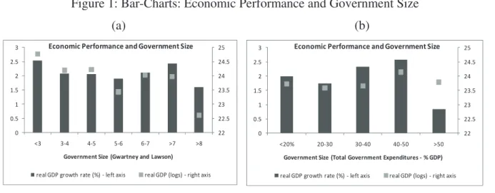
For illustration purposes, Figures 1.a-b and 2.a-b present evidence for a sample of 108

countries supporting the unclear relationship between real GDP (in levels and growth rates)

and two different proxies of government size (the Gwartney and Lawson’s (2008)

composite variable and total government expenditures as share of GDP – see Section 3.1

for details). Hence, there is a need to shed light on this relationship with appropriate

empirical methods.

Figure 1: Bar-Charts: Economic Performance and Government Size

(a) 22 22.5 23 23.5 24 24.5 25 0 0.5 1 1.5 2 2.5 3

<3 3Ͳ4 4Ͳ5 5Ͳ6 6Ͳ7 >7 >8

GovernmentSize(GwartneyandLawson)

EconomicPerformanceandGovernmentSize

realGDPgrowthrate(%)Ͳleftaxis realGDP(logs)Ͳrightaxis

(b) 22 22.5 23 23.5 24 24.5 25 0 0.5 1 1.5 2 2.5 3

<20% 20Ͳ30 30Ͳ40 40Ͳ50 >50

GovernmentSize(TotalGovernmentExpendituresͲ%GDP)

EconomicPerformanceandGovernmentSize

realGDPgrowthrate(%)Ͳleftaxis realGDP(logs)Ͳrightaxis

Source: Authors’ calculations

Figure 2: Scatter-Plots: Economic Performance and Government Size

(a) 0 2 4 6 8 10

Ͳ4 Ͳ2 0 2 4 6 8

G o v e rn m e n t S iz e (G w a rt ne y an d La ws o n )

realGDPgrowth(%)

EconomicPerformanceandGovernmentSize (fullsample)

(b) 0 10 20 30 40 50 60 70

Ͳ4 Ͳ2 0 2 4 6 8

T o ta l G o v e rn m e n t E x p e n d it u re s (% G D P )

realGDPgrowth(%)

EconomicPerformanceandGovernmentSize (fullsample)

Source: Authors’ calculations

The variation of causality between government size and growth detected in

cross-section and time-series papers suggests that there are important differences in the way in

13

which governments influence economic performance across countries. We argue that it

may reflect, lato sensu, institutional differences across countries and, while this is a

plausible conjecture, there is as yet little direct evidence to confirm that institutions and

political regimes make a difference to the way in which governments affect economic

outcomes.

4. Methodology and Results

4.1 Baseline Results

Equations (8) and (9) can be estimated directly using panel data techniques which

allow for both cross-section and time-series variation in all variables and present a number

of advantages vis-à-vis standard Barro-type pooled cross-section estimation approaches

(see Greene, 2003).

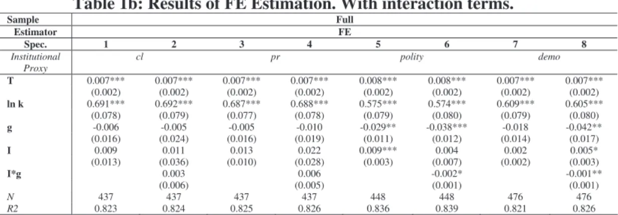
Table 1.a and 1.b present our first set of results for the pooled OLS and fixed-effects

specifications, respectively (the former is presented for completeness). Both tables are

divided into two panels (A and B) covering different proxies for institutional quality (eight

in total). At this point, we use Gwartney and Lawson’s government size measure only and

discuss its individual inclusion in our regression of interest as well as its interaction with a

variable I_it.

[Tables 1.a, 1.b]

A few remarks are worth mentioning. There is a positive effect of the capital stock on

the level of real GDP per capita throughout the different specifications regardless of the

institutional variable employed. One also finds a consistent and statistically significant

negative coefficient on the government size (less so when fixed-effects are used – Table

1.b). Similarly, institutional quality has a consistent and statistically significant positive

impact on the level of real GDP per capita (more mitigated with fixed-effects). Finally,

when statistically significant the interaction term is negative, meaning that i) the negative

effect of government size on GDP per capita is stronger at lower levels of institutional

quality, and ii) the positive effect of institutional quality on GDP per capita is stronger at

smaller levels of government size. The interaction term means that the marginal effect of

government size will differ at different levels of institutional quality. However, this result

depends on the proxy used forI_it. Nevertheless, we obtain in most regressions

considerably high R-squares. Moreover, when regional dummies are included, coefficients

If we redo the exercise with the EMA_PCA variable instead, for both pooled OLS and

fixed-effects estimators, Table 2 shows meaningful results for the size of the government

and for the institutional quality index, when OLS is considered.

[Table 2]

4.2 Endogeneity Issues and Dynamic Panel Estimation

In the analysis of empirical production functions, the issue of variable endogeneity is

generally of concern. Moreover, instead of estimating static equations, we now allow for

dynamics to play a role. Hence, we reformulate our regression equation(s) and take real

GDP growth per capita as our dependent variable being a function of lagged real GDP per

capita, investment (gross fixed capital formation as percentage of GDP), a government-size

proxy and an interaction term (with an institutional quality proxy) – as common practice in

the empirical growth literature. We estimate this new specification by means of the

Arellano-Bover system-GMM estimator14 which jointly estimates the equations in first

differences, using as instruments lagged levels of the dependent and independent variables,

and in levels, using as instruments the first differences of the regressors.15 Intuitively, the

system-GMM estimator does not rely exclusively on the first-differenced equations, but

exploits also information contained in the original equations in levels.

Another novelty of this paper is the construction of new (and more meaningful)

democracy measures based on the variable polity (presented in Section 3 and described in

the Appendix A). The role of political systems and democracy in particular, on the

government size-growth relationship is assessed by regressing three structural aspects of

democracy (to be defined below) on 5-year averages of real GDP per capita growth rates.16

Indeed,politydoes not capture two important dimensions of political regimes - either their

_____________________________ 14

The GMM approach estimates parameters directly from moment conditions imposed by the model. To enable identification the number of moment conditions should be at least as large as the number of unknown parameters. Moreover, the mechanics of the GMM approach relates to a standard instrumental variable estimator and also to issues such as instrumental validity and informativeness.

15

As far as information on the choice of lagged levels (differences) used as instruments in the differences (levels) equation, as work by Bowsher (2002) and, more recently Roddman (2009) has indicated, when it comes to moment conditions (as thus to instruments) more is not always better. The GMM estimators are likely to suffer from “overfitting bias” once the number of instruments approaches (or exceeds) the number of groups/countries (as a simple rule of thumb). In the present case, the choice of lags was directed by checking the validity of different sets of instruments and we rely on comparisons of first stage R-squares.

16

newness (following, for example, democratization or a return to authoritarian rule) or their

more established (consolidated) nature.

Therefore, Rodrik and Wacziarg (2005) define a major political regime change to have

occurred when there is a shift of at least three points in a country’s score on polity over

three years or less. Using this criterion we define new democracies (ND=1) in the initial

year (and subsequent four years) in which a country’s polity score is positive and increases

by at least three points and is sustained, ND=0 otherwise. Established democracies (ED=1)

are those new democratic regimes that have been sustained following the 5 years of a new

democracy (ND). In any subsequent year, if established democracies (ED) fail to sustain

the status of ND, ED=0. Using these criteria, they define sustained democratic transitions

(SDT) as the sum of ND and ED. They use the same procedure, mutatis mutandis, to

define new autocracies (NA), established autocracies (ES) and sustained autocratic

transition (SAT).

This yields six distinct binary-type measures of the character of political regimes - ND,

ED, NA, EA, SDT, and SAT - for most years during 1970-2008. Finally, Rodrik and

Wacziarg (2005) define small regime changes (SM) as changes in polityfrom one year to

the next that are less than three points.17 A recent empirical application of these measures

to explain the impact of extreme-type political regimes on economic performance can be

found in Jalles (2010). There are several advantages from creating these new measures,

which allow us to distinguish the impact of new and established electoral democracies and

autocracies on economic development, and also to assess the impact of sustained

democratic and autocratic transitions on economic growth.

Endogeneity18 between right-hand side measures of democracy and autocracy and a

standard set of control variables is corrected for by taking a system-GMM (SYS-GMM)

approach – as detailed above. As suggested in Mauro (1995), La Porta et al. (1997), Hall

and Jones (1999), Acemoglu et al. (2001) and Dollar and Kraay (2003), the democracy

measures are instrumented by:

1. the durability (age in years) of the political regime type (durable) retrieved from

Marshall and Jaeggers’ database.19

_____________________________ 17

Thus SM = 1 for a small regime change and SM = 0 otherwise.

18

And also the existence of possible measurement errors when accounting for democracy.

19

2. latitude (from La Porta et al., 1999): Hall and Jones (1999) launched the general

idea that societies are more likely to pursue growth-promoting policies, the more

strongly they have been exposed to Western European influence, for historical or

geographical reasons. In this context, other two possible instruments could be

common and civil law, translating the type of legal origin of each different country

(see La Porta et al., 1998).

3. ethnic fragmentation (ethnic) (from Alesina et al., 2003): on a broad level, the role

of ethnic fragmentation in explaining the (possible) growth effect of democracy can

be derived from the literature on the economic consequences of ethnic conflict. It

has been shown that the level of trust is low in an ethnically divided society

(Alesina and La Ferrara, 2000). Moreover, the lack of co-operative behaviour

between diverse ethnic groups, leads to the tragedy of the commons as each group

fights to divert common resources to non-productive activities (e.g. Mauro, 1995).20

Table 3 reports the results with the four proxies for government size defined in Section

3 and splitting the sample into OECD, emerging and developing countries groups.

Focusing on the full sample first we observe that the Gwartney and Lawson’s government

size measure appears with a statistically significant negative coefficient. When interacted

with SAT it has a negative and statistically significant coefficient, meaning that in

autocratic countries increased government size has greater negative effect on output

growth. The reverse is true for democratic countries, whose negative impact of government

size is mitigated but remains mostly negative. The remaining proxies keep the statistically

negative coefficient, but interaction terms lose economic and statistical relevance. For the

OECD sub-group the individual effects of the different proxies of government size are

similar but interaction terms are never statistically significant. Developing countries report

a statistically negative coefficient on government consumption expenditure and

debt-to-GDP ratio, with the latter having a lesser detrimental effect in democratic countries. All in

all, government consumption is the proxy that is more consistently and clearly detrimental

to output growth.

[Table 3]

_____________________________ 20

More stringent empirical tests on the role of democracy on the government size-growth

relation were carried out, for robustness purposes (similarly to Rock, 2009). We defined

“extreme” democratic transitions as those where the polity variable is greater than 5. In

these instances, a new sustainable democratic transitions variable, SDT1 = 1 when polity >

5, otherwise SDT1 = 0. Similarly, a new sustainable autocratic transitions variable was

created, SAT1 = 1 when polity < -5, otherwise SAT1 = 0. The logic behind this

construction is to test for the impact of democracy and autocracy on growth in cases where

countries’ governments are closer to either pure democracies or pure autocracies.21 Results

(not shown) using the new SAT1 and SDT1 variables do not qualitatively change the

results presented in Table 3 and discussed above.

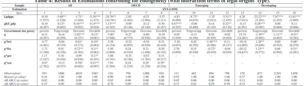
We also assessed the importance of political-institutional measures, specifically legal

origins. From Table 4 a first general conclusion is that interaction terms with a

Scandinavian legal origin dummy yields the higher (in absolute value) estimated

coefficients (when significant), compared with other legal origins. More particularly, in

specification 4 and 5, for the full sample and OECD respectively, the government

debt-to-GDP ratio and government size appear with a (statistically) negative coefficient; however,

this effect on growth is mitigated particularly if a country has a Scandinavian legal origin.

For developing countries, both French and British legal origins appear with statistically

significant positive interaction term coefficients when the government size proxy is total

government expenditures.

[Table 4]

As suggested by Ram (1986) another possible specification is the use of the growth rate

of the government size proxy. We also test this specification to determine its impact on

growth across political systems or levels of institutional quality. All variables are retained

except G_it that is now replaced by dG_it /G_ittogether with the corresponding interaction

term. The results are presented in Table A1 in the Annex. Comparing with our previous

results the coefficients of the linear term of government size proxies (apart from the

debt-to-GDP ratio) are positive and statistically significant in two specifications (2 and 5).

According to Conte and Darrat (1988) Ram’s specification is suitable for testing short-term

growth effects, while the specification used in this paper assesses the effects of government

size on the underlying growth rate. Growth and development are long-run concepts

whereas management of aggregate demand, a Keynesian prescription, is basically a

short-_____________________________ 21

term concept. Hence, while short-term measures of government may have a positive

impact on an economy, the impact of government on the underlying growth rate generally

differs between political regimes and legal origins as found in this paper (a comparable

robustness analysis is reported in Annex Table A2).

Further in our inspection similar regressions, where the I_it variable is now replaced

with the composite Freedom House index, were estimated.22 Two main results are worth

mentioning: i) government size keeps its statistically significant negative sign, but its

interaction with the Freedom House index yields a statistically negative coefficient (for the

full sample), suggesting that the negative effect of government size on GDP per capita

growth is stronger at lower levels of civil liberties and political rights; and ii) for the

OECD sub-group debt has a statistically significant negative coefficient estimate and its

interaction with the Freedom House index results in a negative estimate significant at 5

percent level.

4.3 Fiscal Rules

In the context of the EU, Member States face a fiscal framework that asks for the

implementation of sound fiscal policies, notably within the Stability and Growth Pact

(SGP) guidelines put forward in 1997. In fact, institutional restrictions to budgetary

decision-making are a common feature of fiscal governance in advanced countries (see

Hallerberg et al., 2007 for an overview). In addition to excess spending in the absence of

such rules, previous literature also suggests that the so-called “common pool problem”

may induce a pro-cyclical bias in fiscal policy (Tornell and Lane, 1999). Yet another

rational for the implementation of such fiscal rules is to prevent policymakers from

exacerbating macroeconomic volatility which is known to be detrimental to output growth.

However, the Member States’ track records of effectively implementing fiscal rules have

been mixed.23 Therefore, it is relevant to assess whether such fiscal rules, while aiming at

improving fiscal positions, also play a role in fostering growth, particularly when

interacted with different levels of government size. To our best knowledge such an

empirical exercise has never been conducted.

_____________________________ 22

See Annex Table A3.

23

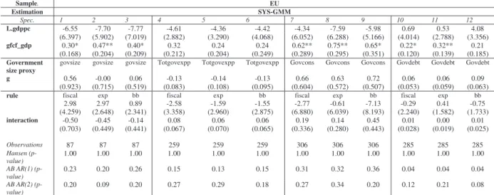
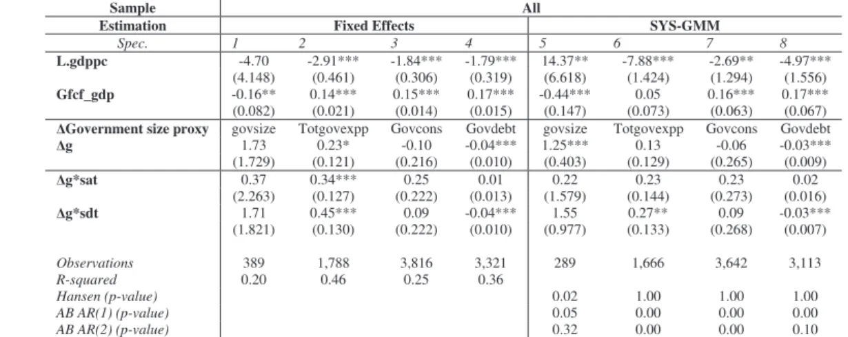
Therefore, we use three indices constructed by the European Commission (overall rule

index, expenditure rule index, and budget balance and debt rule index).24 Tables 5a and 5b

report our findings between 1990-2008 using fixed-effects and system-GMM approaches,

respectively. The former incorporates each index individually whereas the latter includes

interacted terms between fiscal rules and government size proxies.

[Tables 5a, 5b]

Particularly under the total government expenditure and government spending

specifications (4,5, 7, 8) we find statistically significant positive coefficients on the overall

rule index and the expenditure rule index, meaning that having these fiscal numerical rules

improves GDP growth for these set of EU countries. However, the government size proxy

is never significant when these rules are included as additional regressors. When these

rules are interacted with a relevant government size proxy, Table 5b, no coefficient is

statistically significant.

Finally, we also tested specifications with and without interaction terms, and with a

simple splitting rule based on the country-average debt-to-GDP ratio over the entire time

period being higher or lower than 60% (in line with the SGP threshold level). Such

alternative does not change the statistical (in-)significance of our variables of interest

(results not shown).

4.4 Robustness Checks

One concern when working with time-series data is the possibility of spurious

correlation between the variables of interest (Granger and Newbold, 1974). This situation

arises when series are not stationary, that is, they contain stochastic trends as it is largely

the case with GDP and investment series. The advantage of panel data integration is

threefold: firstly, enables to by-pass the difficulty related to short spanned time series;

secondly, the tests are more powerful than the conventional ones: thirdly, cross-section

information reduces the probability of a spurious regression (Barnerjee, 1999).25 Results of

first (Im-Pesaran-Shin, 1997; Maddala-Wu, 1999) and second generation (Pesaran CIPS,

_____________________________ 24

These indices are normalized to have a zero mean and unit variance. They are based on a survey conducted by the Working Group on the Quality of Public Finances among practitioners and researchers in the field of fiscal policy. These measures bear strong appeal for empirical implementations as they translate a broad set of institutional provisions into a country-specific cardinal ranking (see Deburn at al., 2008, and Afonso and Hauptmeier, 2009 for details).

25

2007) panel integration tests are presented in the Annex (Tables A4 and A5).26 We can

accept most conservatively that nonstationarity cannot be ruled out in our dataset.

In face of this finding, it seems that the time-series properties of the data play an

important role: we suggest that the bias in our models is the result of nonstationary errors,

which are introduced into the fixed-effects and GMM equations by the imposition of

parameter homogeneity. Hence, careful modelling of short-run dynamics requires a slightly

different econometric approach. We assume that (8), or (9), represents the equilibrium

which holds in the long-run, but that the dependent variable may deviate from its path in

the short-run (due, e.g., to shocks that may be persistent). There are often good reasons to

expect the long-run equilibrium relationships between variables to be similar across groups

of countries, due e.g. to budget constraints or common technologies (unobserved TFP)

influencing them in a similar way. In fact, in line with discussions in the empirical growth

literature for modelling the “measure of our ignorance” we shall assume that the long-run

relationship is composed of a country-specific level and a set of common factors with

country-specific factor loadings.

The parameters of (8) and (9) can be obtained via recent panel data methods. Indeed, at

the other extreme of panel procedures, based on the mean of the estimates (but not taking

into account that certain parameters may be the same across groups), we have the Mean

Group (MG)27 estimator (Pesaran and Smith, 1995) and as an intermediate approach the

Pooled Mean Group (PMG)28 estimator, which involves both pooling and averaging

(Pesaran et al., 1999). These estimators are appropriate for the analysis of dynamic panels

with both large time and cross-section dimensions, and they have the advantage of

accommodating both the long-run equilibrium and the possibly heterogeneous dynamic

adjustment process.

Therefore, a second step in our empirical approach is to make use of the Common

Correlated Effects Pooled (CCEP) estimator that accounts for the presence of unobserved

common factors by including cross-section averages of the dependent and independent

variables in the regression equation and where averages are interacted with

country-dummies to allow for country-specific parameters. In the heterogeneous version, the

_____________________________ 26

For further details on these tests, the interested reader should refer to the original sources.

27

The MG approach consists of estimating separate regressions for each country and computing averages of the country-specific coefficients (Evans, 1997; Lee et al., 1997). This allows for heterogeneity of all the parameters.

28

Common Correlated Effects Mean Group (CCEMG), the presence of unobserved common

factors is achieved by construction and the estimates are obtained as averages of the

individual estimates (Pesaran, 2006). A related and recently developed approach due to

Eberhardt and Teal (2010) was termed Augmented Mean Group (AMG) estimator and it

accounts for cross-sectional dependence by inclusion of a “common dynamic process”.29

We base our panel analysis on the unrestricted error correction ARDL(p,q)

representation: T t N i u x y x y

y i it

q q j it ij p j j it ij it i it i

it ' ' , 1,2,..., ; 1,2,...,

1

1 1

1 1

1 ' '

' I E

¦

¦

where y_itis a scalar dependent variable, x_it is the ku1 vector of regressors for group i,

i

P represents the fixed effects, I_iis a scalar coefficient on the lagged dependent variable.

i

'

E ’s is the ku1vector of coefficients on explanatory variables, O_ij’s are scalar

coefficients on lagged first-differences of dependent variables, and J_ij’s are ku1

coefficient vectors on first-differences of explanatory variables and their lagged values. We

assume that the disturbances u_it’s in the ARDL model are independently distributed across

i and t, with zero means and constant variances. Assuming that I_i 0for all i, there exists

a long-run relationship between yitand xit defined as:

T t

N i

y

y_it T'_{i it1}K_it, 1,2,..., ; 1,2,..., (11)

where T'_i E_i'/I_iis the ku1 vector of the long-run coefficients, and K_it’s are stationary with possible non-zero means (including fixed effects). Equation (10) can be rewritten as:

T t N i u x y

y _{i it}

q q j it ij p j j it ij it i

it ' , 1,2,..., ; 1,2,...,

1

1 1

1

1 ' '

' IK

¦

¦

where K_it1is the error correction term given by (11), hence I_i is the error correction

coefficient measuring the speed of adjustment towards the long-run equilibrium.

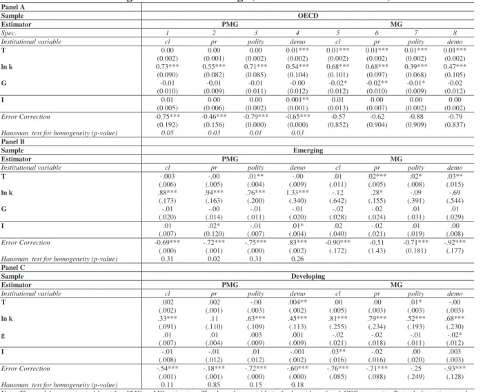
Table 6.a presents our first set of robustness results, and it includes for each sub-sample

both the PMG and MG estimates using different proxies for institutional quality entering in

linear form together with the Gwartney and Lawson government size variable. For the

OECD sub-group we get a positive and statistically significant coefficient on democracy in

specification 4 and three statistically negative coefficients of government size when using

the MG estimator. For both emerging and developing countries (Panels B and C) statistical

_____________________________ 29

significance of government size is hard to find, but the institutional proxy is statistically

significant for emerging countries (pr, political rights, and democracy), and for developing

countries (cl, civil liberties).

[Table 6.a]

The MG estimator provides consistent estimates of the mean of the long-run

coefficients, though these will be inefficient if slope homogeneity holds. Under long-run

slope homogeneity, the pooled estimators are consistent and efficient. The hypothesis of

homogeneity is tested empirically in all specifications using a Hausman-type test applied to

the difference between MG and PMG. Under the null hypothesis the difference in the

estimated coefficients between the MG and the PMG estimators is not significant and the

PMG is more efficient. The p-value of such a test is also present in Table 6.a, and only for

the OECD the null is rejected, being the MG estimator more efficient, and the long-run

slope homogeneity rejected.

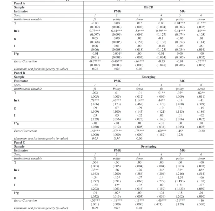
In Table 6.b an equivalent set of results is presented but now with the integration term

between government size and an institutional proxy of interest. In the case of the OECD

the interaction term is negative and statistically significant for the polity indicator instance.

However, the government size is not significant. In the case of developing countries, with

the polity variable, government size negatively affects the level of per capita GDP,

institutional quality appears with positive and statistically significant estimate and, we get

a negative interaction coefficient. All in all, results using either PMG or MG estimators do

not present extremely consistent evidence on the interactive effect of our variables of

interest on the output level.

[Table 6.b]

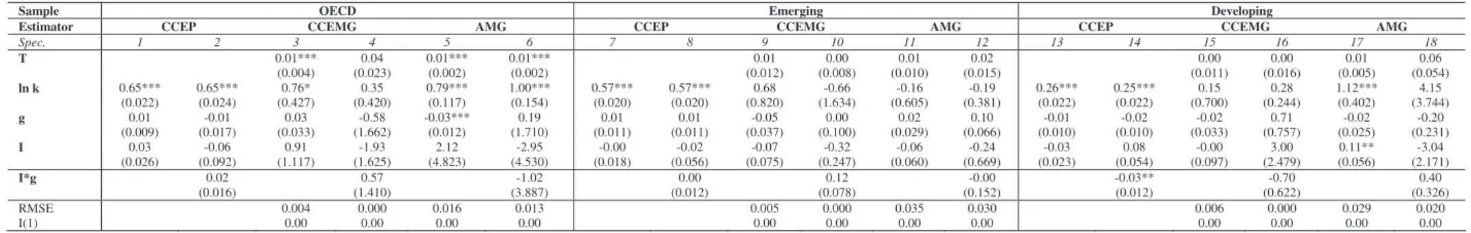
In Table 7 we allow for both heterogeneous technology parameters and factor loadings

as explained above, by running the CCEP, CCEMG and AMG estimators with and without

interaction terms (where the institutional proxy variable is now given by the EMA_PCA

variable as explained in Section 3). When running the AMG estimator for the OECD group

we find some evidence of a statistically significant negative coefficient on the government

size variable; while for the developing countries group we uncover only one statistically

significant positive coefficient on the EMA-PCA variable, across methods.

[Table 7]

We redo the exercise but similarly to Tables 3 and 4 allow for other proxies of

government size to play a role (see Table 8). Only estimated coefficients of the

term are reported for reasons of parsimony (full results are available upon request). We

present different econometric specifications mainly for robustness and completeness. All in

all, we get negative and statistically significant coefficients on total government

expenditure, government consumption and public debt-to-GDP ratio irrespectively of the

sample under scrutiny. We refrain from making a detailed analysis. Still, for instance,

specifications 7 and 11 for the emerging and developing countries groups and with the

government consumption as a proxy for government size show a negative effect of

government consumption, and a positive effect of the PCA-based institutional measure.

Finally, there is a negative interaction term: i) the negative effect of government

consumption on GDP per capita is stronger at lower levels of institutional quality, and ii)

the positive effect of institutional quality on GDP per capita increases at smaller levels of

government consumption.

[Table 8]

5. Conclusion

We constructed a growth model with an explicit government role showing that more

resources required to finance government spending reduce both the optimal level of private

consumption and of output per worker. Following up on that theoretical motivation we

perform an empirical panel analysis with 108 countries from 1970-2008, employing

different proxies for government size and institutional quality.

This paper adds to the literature in providing evidence on the issue of whether “too

much” government is good or bad for economic progress and macroeconomic

performance, particularly when associated with differentiated levels of (underlying)

institutional quality and alternative political regimes.

Moreover, we make use of recent panel data techniques that allow for the possibility of

heterogeneous dynamic adjustment around the long-run equilibrium relationship as well as

heterogeneous unobserved parameters and cross-sectional dependence (e.g. Pooled Mean

Group, Mean Group, Common Correlated Pooled estimators, inter alia); vi) we also deal

with potentially relevant endogeneity issues.

Our results allow us to draw several conclusions regarding the effects on economic

growth of the size of the government: i) there is a significant negative effect of the size of

government on growth; ii) institutional quality has a significant positive impact on the

level of real GDP per capita; iii) government consumption is consistently detrimental to

developing countries); iv) moreover, the negative effect of government size on GDP per

capita is stronger at lower levels of institutional quality, and the positive effect of

institutional quality on GDP per capita is stronger at smaller levels of government size.

Therefore, our empirical results are consistent with the growth model presented in the

paper.

In addition, the negative effect on growth stemming from the government size

variables is more attenuated for the case of Scandinavian legal origins, while the negative

effect of government size on GDP per capita growth is stronger at lower levels of civil

liberties and political rights.

Finally, and for the EU countries, we find statistically significant positive coefficients

on overall fiscal rule and expenditure rule indices, meaning that having better fiscal rules

in place improves GDP growth.

References

1. Abas, A., Belhocine, N., El Ganainy, A., Horton, M. (2010), “A Historical Public Debt

Database”, IMF Working Paper No. 10/245.

2. Acemoglu, D. and Robinson, J. (2005), "Economic Origins of Dictatorship and

Democracy", Cambridge University Press.

3. Acemoglu, D., Johnson, S. and Robinson, J.A. (2001),"The colonial origins of

comparative development: an empirical investigation", American Economic Review,

91, 1369.1401.

4. Afonso, A.; Schuknecht, L., Tanzi, V. (2005). “Public Sector Efficiency: an

International Comparison,” Public Choice, 123 (3-4), 321-347.

5. Afonso, A., Schuknecht, L. Tanzi, V. (2011). “Income Distribution Determinants and

Public Spending Efficiency”, Journal of Economic Inequality, 8 (3), 367-389.

6. Afonso, A. and Hauptmeier, S. (2009). “Fiscal behaviour in the EU: rules, fiscal

decentralization and government indebtedness”, ECB WP 1054.

7. Alesina, A. and La Ferrara, E. (2000), "The Determinants of Trust", NBER Working

Papers 7621.

8. Alesina, A., Devleeschauwer, A., Easterly, W., Kurlat, S., and Wacziarg, R. (2003),

“Fractionalization.” Journal of Economic Growth, 8, 155-194.

9. Bajo-Rubio, O. (1991), “A further generalization of the Solow growth model: the role

of the public sector”, Economic Letters, 68, 79-84.

10. Banerjee, A. (1999), “Panel data, unit roots and cointegration: an overview”, Oxford

Bulletin of Economics and Statistics, Special Issue on Testing Unit Roots and Cointegration using Panel Data, Theory and Applications, 61, November, 607-629.

11. Barro, R. (1991), “Economic growth in a cross section of countries”, Quarterly

Journal of Economics, 106, 407-443.

12. Barro, R. and Sala-i-Martin, X. (1992), “Convergence”, Journal of Political Economy,

13. Beck, T., Clarke, G., Groff, A., Keefer, P. and Walsh, P. (2001), “New tools and new

tests in comparative political economy: the Database of Political Institutions”, World

Bank Economic Review 15, 165-176.

14. Bockstette, V, Chanda, A. and Putterman, L. (2002), " States and Markets: The Advantage of an Early Start", Journal of Economic Growth, 7(4), 347-69.

15. Browsher, C. G. (2002), “On testing overidentifying restrictions in dynamic panel data models”, CEPR Discussion Paper No. 3048, CEPR London.

16. Coakley, J., Fuertes, A.M. and Smith, R. (2006), “Unobserved heterogeneity in panel

time series models”, Computational Statistics and Data Analysis 50(9), 2361–2380.

17. Conte, M.A., and A.F. Darrat (1988), “Economic Growth and the Expanding Public Sector”, Review of Economics and Statistics, 322-330.

18. Dalamagas, B. (2000), “Public sector and economic growth: the Greek experience”,

Applied Economics, 32, 277-288.

19. Debrun, X., Moulin, L., Turrini, A., Ayuso-i-Casals, J. And Kumar, M. (2008). “Tied to the mast? National Fiscal rules in the EU”, Economic Policy, 23(54), 297-362. 20. Dempster, A. P., N. M. Laird, and D. B. Rubin (1977), “Maximum likelihood from

incomplete data via the EM algorithm”, Journal Royal Statistical Society B, 39, 1–22, 1977.

21. Dollar, D. and Kraay, A. (2003), "Institutions, trade and growth", Journal of Monetary Economics, 50, 133.162.

22. Dupuit, Jules (1844). “De la Mesure de l’Utilité des Travaux Publiques”, Annales des

Ponts et Chaussées. 8. Translated and reprinted in: Kenneth Arrow and Tibor Scitovski (eds.), 1969, AEA Readings in Welfare Economics, AEA: 255-283.

23. Easterly, W. R. (2001), “The Lost Decades: Developing Countries Stagnation in Spite

of Policy Reform 1980-1998”, Journal of Economic Growth, 6(2), 135-157.

24. Eberhardt, M., and Teal, F. (2010), “Productivity Analysis in Global Manufacturing Production”, Oxford University, Department of Economics Discussion Paper Series #515, November 2010.

25. European Commission (2006). “Public Finances in EMU”, European Economy, 3.

26. Evans, P. (1997), “How fast do economies converge”, Review of Economics and

Statistics, 46, 1251-1271.

27. Fölster, Stefan; and Magnus Henrekson. 2001. "Growth effects of government

expenditure and taxation in rich countries", European Economic Review 45,

1501-1520.

28. Friedman, M. (1997), “If only the US were as free as Hong Kong”, Wall Street Journal, July 8, A14.

29. Ghali, K. H. (1998), “Government size and economic growth: evidence from a multivariate cointegration analysis”, Applied Economics, 31, 975-987.

30. Granger, C. W. J. And Newbold, P. (1974), “Spurious regressions in econometrics”,

Journal of Econometrics, 2, 111-120.

31. Greene, W. (2003), “Econometric Analysis”, Pearson Education Inc., New Jersey 32. Guseh, J. S. (1997), “Government size and economic growth in developing countries: a

33. Gwartney, J., and Lawson, R.A. (2008), “Economic Freedom of the World: 2008 Annual Report” http://freetheworld.com/

34. Hall, R.E. and Jones, C. (1999), “Why do some countries produce so much more

output per worker than others?” Quarterly Journal of Economics, 114, 83.116.

35. Hallerberg, M., Strauch, R. and von Hagen, J. (2007). “The design of fiscal rules and

forms of governance in EU countries”, European Journal of Political Economy, 23,

338-359.

36. Im, K. S., Pesaran, M. H. and Shin, Y. (2003), “Testing for unit roots in heterogeneous

panels,”Journal of Econometrics 115, 53– 74..

37. IMF (2001), “A Manual on Government Finance Statistics 2001”, (GFSM 2001), http://www.imf.org/external/pubs/ft/gfs/manual/gfs.htm Washington DC: International Monetary Fund.

38. Jalles, J. T. (2010), “Does democracy foster or hinder growth? Extreme-type political regimes in a large panel," Economics Bulletin, 30(2), 1359-1372.

39. Kapetanios, G., Pesaran, M. H., & Yamagata, T. (2011), “Panels with Nonstationary Multifactor Error Structures”, Journal of Econometrics, 160 (2), 326-348.

40. Kaufmann, D., Kraay, A. and Mastruzzi, M. (2009),. “Governance Matters VIII: Aggregate and Individual Governance Indicators for 1996–2008”, World Bank Policy Research Paper No. 4978. http://ssrn.com/abstract=1424591

41. La Porta, R., Lopez-de-Silanes, F., Shleifer, A., and Vishny, R. (1997), "Legal determinants of external finance", Journal of Finance, 52, 1131-1150.

42. La Porta, R., Lopez-de-Silanes, F., Shleifer, A., and Vishny, R. (1998), "Law and finance",Journal of Political Economy, 106, 1113-1155.

43. La Porta, R., López-de-Silanes, F., Shleifer, A.. and Vishny, R. (1999), The Quality of

Government. Journal of Law, Economics and Organization, 15(1), 222-279.

44. Lee, K., Pesaran, M. H. And Smith, R. P. (1997), “Growth and convergence in a

multi-country empirical stochastic Solow model”, Journal of Applied Econometrics, 12,

357-392.

45. Little J.A., Rubin D.B. (1987), “Statistical Analysis with Missing Data”, John Wiley and Sons, New York

46. Maddala, G. S. and Wu, S. (1999), “A comparative study of unit root tests with panel

data and a new simple test”, Oxford Bulletin of Economics and Statistics, 61,

November, 631-652.

47. Mankiw, N. G., Romer, D. And Weil, D. N. (1992), “A contribution to the empirics of

economic growth”, Quarterly Journal of Economics, 107, 407-437.

48. Mauro, P. (1995), "Corruption and growth", Quarterly Journal of Economics, 110,

681.712.

49. Nelson, R. R. and Sampat, B.N. (2001), “Making sense of institutions as a factor

shaping economic performance”, Journal of Economic Behavior and Organization, 44,

31-54.

50. North, D. (1990), “Institutions, Institutional Change and Economic Performance”, Cambridge: Cambridge University Press.

52. Pesaran, M. H. (2007), “A simple panel unit root test in the presence of cross section dependence”, Journal of Applied Econometrics, 22(2), 265-312.

53. Pesaran, M. H. and Smith, R. P. (1995),“Estimating long-run relationship from

dynamic heterogeneous panels”, Journal of Econometrics, 68, 79-113.

54. Pesaran, M. H., Shin, Y. and Smith, R. P. (1999), “Pooled mean group estimation of

dynamic heterogeneous panels”, Journal of American Statistical Association, 94,

31-54.

55. Poterba, James M (1996), "Budget Institutions and Fiscal Policy in the U.S. States",

American Economic Review, 86(2), 395-400.

56. Przeworski, A., Alvarez, M., Cheibub, J., Limongi, F. (2000), "Democracy and Development: Political regimes and economic well-being in the World, 1950-1990", New York: Cambridge University Press.

57. Ram, R. (1986), “Government Size and Economic Growth: a New Framework and

Some Evidence from Cross-section and Time Series Data”, American Economic

Review, 76, 191-203.

58. Rock, M. (2009), "Has Democracy Slowed Growth in Asia?", World Development,

37(5), 941-952.

59. Rodrik, D., and R. Wacziarg (2005), “Do Democratic Transitions Produce Bad

Economic Outcomes?", American Economic Review, 95(3), 50-55.

60. Roodman, D. M. (2009), “A note on the theme of too many instruments”, Oxford

Bulletin of Economics and Statistics, 71(1), 135-58.

61. Rousseeuw, P.J. and K. Van Driessen (1999), “A fast algorithm for the minimum

covariance determinant estimator”, Technometrics, 41, 212–223.

62. Slemrod, J. (1995), “What do cross-country studies teach about government

involvement, prosperity, and economic growth?”, Brookings Papers on Economic

Activity, 2, 373-431.

63. Tanzi V. and H. Zee (1997), “Fiscal policy and long-run growth”, IMF Staff Papers,

44, 179-209.

64. Tornell, A. and Lane, P. R. (1999). “The voracity effect”, American Economic Review,

89, 22-46.