Bio-Measurements Estimation and Support in Knee Recovery through Machine Learning

F

E

U

P

Bio-Measurements Estimation and

Support in Knee Recovery through

Machine Learning

João Miguel Neves Bernardino

Mestrado Integrado em Engenharia Informática e Computação Supervisor: Hugo Sereno Ferreira, PhD

Second Supervisor: Luís Filipe Teixeira, PhD External Advisor: Fábio Rocha, Physical Therapist

c

João Miguel Neves Bernardino, 2018 All Rights Reserved

Bio-Measurements Estimation and Support in Knee

Recovery through Machine Learning

João Miguel Neves Bernardino

Mestrado Integrado em Engenharia Informática e Computação

Approved in oral examination by the committee:

External Examiner: Prof. Pedro Ribeiro Supervisor: Prof. Hugo Sereno Ferreira

Abstract

The knee is the most complex joint of the human body, having multiple ligaments and tendons in its composition. As a consequence, many distinct injuries can occur, often requiring the patient to undergo intensive rehabilitation during several months. Regardless of the exact nature of the injury, treatment protocols usually contemplate some recurrent measurements and evaluations that provide valuable information for enhancing the rehabilitation process. Unfortunately, due to the high cost of some required equipment or the fact that some of these procedures are complex and time-consuming, they are often neglected.

A deep learning based solution for performing measurements of knee range of motion using convolutional neural networks is presented, supported by the generation of a synthetic dataset. A 3D human-body model was used to generate realistic and varied images, perpendicular to the plane defined by the lower limb, simulating a patient lying pronate on a treatment table with the leg flexed at arbitrary angles. Such images were labeled, being registered the coordinates of three key points for the calculation of the flexion angle: the centers of the thigh, the knee and the lower leg. This data was used to train convolutional neural networks for performing regression and predicting these six coordinates. Transfer learning was used with the VGG16 and InceptionV3 models pre-trained on the ImageNet dataset. An additional custom model was trained from scratch. These networks were tested under various conditions using different combinations of image augmentation techniques on the training sets. Out of the three architectures, Eva achieved the best results, closely followed by InceptionV3. VGG16’s results were unsatisfactory. Posterior testing was performed using a few real images to test how well the network generalized, and the results were also favorable.

Future work would involve further improvement of the solution and its integration in a mobile application which could be used by physiatrists and physical therapists, providing a superior level of usability in comparison to current methods used for this type of measurement, ultimately optimizing the rehabilitation process.

CCS Concepts: Computing methodologies → Artificial intelligence → Computer vision → Computer vision problems → Object recognition

Keywords: knee, rehabilitation, measurements, goniometry, range of motion, physical therapy, computer vision, machine learning, deep learning, convolutional neural networks, smartphone, camera

“Whether you think you can or think you can’t, you’re right.”

Contents

2 State of the Art 5 2.1 Measurements in Knee Rehabilitation . . . 5

2.1.1 Goniometry . . . 5 2.2 Smartphone-based Solutions . . . 7 2.2.1 Inertial-based goniometry . . . 7 2.2.2 Photography-based goniometry . . . 8 2.3 Conclusion . . . 9 3 Background 11 3.1 Image Recognition . . . 11 3.1.1 Computer vision . . . 11 3.1.2 Machine learning . . . 12 3.1.3 Deep learning . . . 12

3.1.4 Convolutional neural networks . . . 12

3.2 Transfer Learning . . . 14

3.3 Deep Learning with Synthetic Data . . . 14

3.4 Supporting Frameworks and Software . . . 14

3.4.1 MakeHuman . . . 14 3.4.2 Blender . . . 15 3.4.3 Keras . . . 16 3.4.4 CoreML . . . 16 3.5 Conclusion . . . 16 4 Problem Statement 17 4.1 Requirements . . . 17 4.2 Solution Proposal . . . 18 4.3 Evaluation . . . 18 4.4 Conclusion . . . 18

5 Synthetic Dataset Generation 21 5.1 3D Model Creation . . . 21

CONTENTS

5.3 Automated Data Generation . . . 23

5.4 Conclusion . . . 25

6 Image Recognition 27 6.1 Supporting Libraries and Resources . . . 27

6.2 Image Augmentation . . . 28 6.3 CNN Architectures . . . 30 6.3.1 InceptionV3 . . . 31 6.3.2 VGG16 . . . 32 6.3.3 Eva . . . 32 6.4 Training . . . 33 6.4.1 Test #1: No augmentation . . . 35

6.4.2 Test #2: Horizontal flips . . . 36

6.4.3 Test #3: Translations . . . 37

6.4.4 Test #4: Background images . . . 38

6.4.5 Test #5: Rotations . . . 39

6.4.6 Test #6: Flips and translations . . . 40

6.4.7 Test #7: Flips, translations and rotations . . . 41

6.4.8 Test #8: Flips, translations, rotations and backgrounds . . . 42

6.5 Conclusion . . . 43

7 Conclusions 45 7.1 Difficulties . . . 46

7.2 Future Work . . . 46

7.2.1 Diversity of the dataset . . . 46

7.2.2 Different CNN architectures . . . 46

7.2.3 Predicting vectors instead of points . . . 47

7.2.4 Predicting the flexion angle directly . . . 47

7.2.5 Mobile application . . . 47 7.2.6 On-site validation . . . 47 7.2.7 Augmented reality . . . 47 7.2.8 Additional measurements . . . 48 7.3 Epilogue . . . 48 References 49 vi

List of Figures

1.1 Anatomy of the human knee . . . 2

2.1 Measurement of joint angle in x-ray . . . 6

2.2 Universal goniometer . . . 6

2.3 Digital protractor . . . 7

2.4 Knee goniometry using a gyroscope-based application . . . 8

2.5 Knee ROM measured with DrGoniometer . . . 9

3.1 Typical structure of a CNN . . . 13

3.2 MakeHuman’s main interface . . . 15

3.3 Blender’s main interface . . . 15

5.1 MakeHuman 3D models . . . 22

5.2 Different knee flexion angles in Blender . . . 23

5.3 Examples of different skin textures used . . . 23

5.4 Examples of synthesized data . . . 24

6.1 Examples of the transformations applied to the dataset . . . 28

6.2 Some of the photographs used as background . . . 29

6.3 Diagram representing the required CNN structure . . . 31

6.4 Samples from the validation sets . . . 34

6.5 Training curves for Test #1 . . . 35

6.6 Sample predictions after Test #1 . . . 35

6.7 Training curves for Test #2 . . . 36

6.8 Sample predictions after Test #2 . . . 36

6.9 Training curves for Test #3 . . . 37

6.10 Sample predictions after Test #3 . . . 37

6.11 Training curves for Test #4 . . . 38

6.12 Sample predictions after Test #4 . . . 38

6.13 Training curves for Test #5 . . . 39

6.14 Sample predictions after Test #5 . . . 39

6.15 Training curves for Test #6 . . . 40

6.16 Sample predictions after Test #6 . . . 40

6.17 Training curves for Test #7 . . . 41

6.18 Sample predictions after Test #7 . . . 41

6.19 Training curves for Test #8 . . . 42

6.20 Sample predictions after Test #8 . . . 42

6.21 InceptionV3 predictions on edited photographs (background removed) . . . 43

LIST OF FIGURES

List of Tables

5.1 Example of data stored in the CSV file . . . 24

6.1 InceptionV3 final fully-connected layers (modified) . . . 31

6.2 VGG16 final fully-connected layers (modified) . . . 32

6.3 Layers of the Eva CNN model . . . 33

6.4 Results of the 8 test scenarios. T and V columns represent the minimum loss values on the training and validation sets, respectively. Lower results are better. . . 43

LIST OF TABLES

Abbreviations

ACL Anterior cruciate ligament CNN Convolutional neural network CSA Cross-sectional area

DL Deep learning

IT Information technology ML Machine learning ROM Range of motion UG Universal goniometer

Chapter 1

Introduction

The main purpose of this first chapter is to provide some insight on the problem that is in the origin of this project. Section1.1contains a brief description of its context. Sections1.2and1.3

respectively explain the reasons for exploring a novel and different solution to the problem and the expected outcome of this work. Lastly, in section1.4, the structure of this document is reviewed in detail.

1.1

Context

The knee is the largest and most anatomically complex joint in the human body [GR03]. It is formed between three bones and contains multiple tendons and ligaments, as seen on figure 1.1. Its complicated structure, combined with the great amount of stress caused by the forces it is subject to, makes it one of the most frequently injured joints, especially among athletes. A study published in 2006 revealed that, from 19.530 sports injuries documented over a 10-year period, close to 40% were related to the knee [MSK06].

The most common types of injury usually involve ruptures, either partial or complete, of some structure of the knee, such as cartilage, ligaments or tendons. In a great number of cases, especially the ones involving complete ruptures, surgical intervention might be necessary. Since the soft structures of the knee are very delicate, post-operative recovery time is usually long. For instance, an athlete who suffers an anterior cruciate ligament (ACL) full tear, which is one of the most

Introduction

Figure 1.1: Anatomy of the human knee [Sin88]

frequent sports-related knee injuries, may be forced to halt his or her activity for six months or more. During this period, it is highly recommended that patients enroll in a physical therapy program, as a good rehabilitation is absolutely crucial for a successful recovery.

1.2

Motivation

It is the responsibility of the physiatrist to guide the physical therapy program, evaluating the patient’s condition and adjusting the exercises and procedures accordingly. When it comes to knee rehabilitation, the protocol is quite similar for most injury types, with great focus on restoring the joint’s full function, including range of motion (ROM), and regaining muscle mass [PB07]. Joint inflammation following the injury, or even the surgical intervention itself, may cause (and usually does) some limitation of the ROM. And since the patient has to temporarily refrain from exerting load on the injured leg, if not completely immobilize it, muscle atrophy is usually inevitable following a knee injury [KJR+07].

Given that not all patients have the same requirements or recover at the same pace, the reha-bilitation programs should be as adaptive as possible to their needs. That can only be achieved through frequent assessment and evaluation by the health care professional, mostly the physiatrist. Ideally, there should be a balance between both quantitative and qualitative evaluation. While the first is more detailed and provides more insight on the patient’s current status, it is generally harder to perform. Some accurate measurements are time-consuming or can only be performed using expensive specific equipment that not all clinics have available.

Introduction

Thus, in most cases, the evaluation is mainly qualitative, based on not-so-accurate visual estimations, and also not very frequent. This work is supported by the idea that an easier and quicker way to perform meaningful measurements would contribute to an increased amount of evaluations performed, as well as a deeper insight on the patient’s progress.

1.3

Goals

This project’s main goal is the creation of a mobile application capable of performing accurate measurement of the knee’s range of motion. It should be a low-cost solution that is simple and quick enough to operate, so that physical therapists, even more that physiatrists, can use it frequently, as they are the professionals that most closely follow and deal with the patient during the treatment.

Specifically, the app should be capable of estimating the joint’s flexion angle using a common smartphone’s camera. The estimations should be executed in real-time, without requiring photogra-phy or any interaction by the professional other than pointing the camera, and the obtained results should promptly be presented on the device’s screen.

1.4

Report Structure

This introduction is followed by seven more chapters. The next one consists of a detailed review of state of the art solutions currently aiding the rehabilitation process of knee injuries. Chapter3

presents a theoretical background relevant to this dissertation. Chapter4is the problem statement, where the proposed solution is described in detail, followed by a work plan. Chapters5and6go through the technical details of the implementation of the solution. And, lastly, chapter7concludes with a brief summary and a discussion of possible follow-up work in the future.

Introduction

Chapter 2

State of the Art

2.1 Measurements in Knee Rehabilitation . . . 5 2.2 Smartphone-based Solutions . . . 7 2.3 Conclusion . . . 9

This chapter is a detailed revision of state-of-the-art tools related to the problem being addressed in this report. It starts with a broad revision of the measurements described in section1.3and the techniques or tools used to perform them, followed by a more detailed analysis regarding low-cost alternatives based on smartphones.

2.1

Measurements in Knee Rehabilitation

While there is a wide variety of measurements and tests that are relevant to the treatment and recovery of knee injuries, the scope of this project is focused on goniometry — the medical term that refers to the measurement of range of motion of a joint.

2.1.1 Goniometry

The measurement of the range of motion of the knee is a recurrent task in knee rehabilitation which can be achieved using a variety of methods or tools. It is conducted by determining the angle described by two lines representing the axis of the femur and the axis of the fibula, respectively [GBRN87]. The technique generally accepted as reference consists of direct observation of the bones in a radiograph [EGD+04], as seen in figure2.1.

Since knee goniometry should be performed frequently during the rehabilitation, using the radiographic method is not feasible due to radiation exposure. Alternatively, multiple tools were

State of the Art

Figure 2.1: Measurement of joint angle in x-ray [NKA+11]

created in order to enable this procedure [HDM49]. Currently, the universal goniometer, depicted in figure2.2, is the one most commonly used. With more than 30 degrees of knee flexion, there is no significant difference between the results obtained using this method and the radiographic one [Enw86].

Figure 2.2: Universal goniometer [RSJSL13]

While using this tool is considered one of the most reliable methods, this approach has some disadvantages. First of all, it requires a specific device, which might not be available at every physical therapy clinic. Furthermore, its usage requires manual manipulation by the expert. On the one hand, this introduces some error to the estimation. Thus, it is advisable that all measurements on a patient be performed by the same person [HDM49]. On the other hand, this method can only be used while the patient’s injured leg is in a static position. It provides no way to measure the angles of the knee during motion, such as walking or running on the treadmill.

Another device that can be used to measure joint angles is a digital inclinometer, or protractor. This works in the same fashion as a common bubble inclinometer, but reports the actual value of the inclination in degrees. Unlike the universal goniometer, this tool doesn’t immediately reveal the angle of the joint. Instead, both the inclination of the thigh and the lower leg must be measured. Then, the desired value can be obtained by subtracting these two. As well as being a bit more complex to use, this device is also more expensive than a universal goniometer. However, in terms of reliability and validity, the two approaches are similar [KH12].

1_{Source:https://www.msi-viking.com/Mitutoyo-950-318-Pro-360-Digital-Protractor-Output_p_22350.html}

State of the Art

Figure 2.3: Digital protractor1

Furthermore, a study published in 1985 concluded that goniometry could be performed with greater accuracy using photography than with standard tools [FW85]. However, it was only a few years later that this approach was practical, thanks to the advances in digital photography. In order to establish the angle of the joint to be measured, two techniques are used. One uses adhesive skin markers that are manually placed on the patient’s leg, while the other requires the estimations of the lines of the femur and the fibula, much like in the radiographic approach. Both strategies yield similar consistency and accuracy when compared to using x-rays [NKA+11], even considering the estimations done by the expert regarding the angle described by the joint, either when placing the markers or drawing bone lines. One major disadvantage of photography-based goniometry is the necessity of using software to obtain the actual measurement from the captured image. While the results can indeed have great accuracy, errors can easily be introduced by using inappropriate procedures. For instance, the photography should be taken from a perpendicular viewpoint and centered in the angle being measured [DCG06].

2.2

Smartphone-based Solutions

Nowadays, information technology (IT) has advanced to a point where mobile communication and portable computation can be combined on a single device known as smartphone. Most of these are packed with a diverse set of sensors, including digital cameras, magnetometers and accelerometers. This makes these devices quite suitable for a huge variety of applications and purposes, including health care. Whether it aids the retrieval of information, supports diagnosis or provides any other kind of solution, the use of smartphones in medicine is growing at a quick pace [MYS12].

The following sections present recent smartphone-based solutions to the problems being approached in this project.

2.2.1 Inertial-based goniometry

An inertial sensor that is present in most smartphones is the gyroscope. This component relies on Earth’s gravity to determine the orientation, and it is usually calibrated to read a value of 0o when the device is on a horizontal position. Thus, a gyroscope-equipped smartphone can provide the same functionality as a digital inclinometer, making it suitable to perform goniometry. Again, this technique also requires the measurement of two inclinations (thigh and lower leg) before

State of the Art

determining the joint’s angle, as depicted in figure2.4. There are some applications developed specifically for the purpose of goniometry that simplify this process. One of the first apps to be scientifically evaluated is iGoniometer (which is no longer available). The study compared this application with a long arm goniometer2and concluded that the difference in accuracy was low enough so that it would not have a negative clinical impact [HSO12].

Figure 2.4: Knee goniometry using a gyroscope-based application [Jen13]

A study evaluating a different mobile application, performing knee goniometry at six different leg positions (full extension, 30o, 60o, 90o, 110oand maximal flexion), indicates a slightly higher accuracy of this measurement technique when compared to conventional ones [Jen13]. Previous research demonstrates that this approach is precise enough to be frequently used in a clinical environment. Moreover, there are multiple similar applications available for free, making this an inexpensive solution for performing knee goniometry (excluding the cost of the smartphone).

2.2.2 Photography-based goniometry

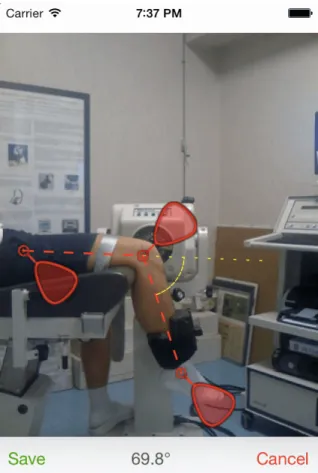
DrGoniometer is a mobile application that is capable of measuring the angles of the patient’s articulations. It uses a photography-based approach, thus being appropriate for static joint angle measurement only. As it was earlier mentioned, in order to get an accurate estimate the camera’s point of view should be parallel to the plane defined by the leg [FVS+13]. Doing so will avoid errors induced by perspective distortion. It’s worth noting that this rule is not specific to DrGoniometer, but rather any photography-based angle measurement system.

In this particular case, after taking a picture, three markers must be dragged to the appropriate positions. Recommended reference points are the center of the knee, the hip and the ankle [FVS+13]. Having these three markers positioned, the application presents two dashed lines representing the angle of the joint, and the measured value is visible on the bottom of the screen. Using the coordinates of the markers, the angle calculation is based on simple trigonometry.

Regarding this particular solution, studies have been published demonstrating its reliability and validity, not only for measuring knee range of motion, but also other joints of the human body [OAB+15]. The results reveal measurement errors similar to those of traditional measurement tools,

2_{A device similar to the universal goniometer}

State of the Art

Figure 2.5: Knee ROM measured with DrGoniometer

such as the Universal Goniometer, making it a perfectly valid solution to be used by professionals [FVS+13].

2.3

Conclusion

This chapter explained one of the most common measurement tasks when treating knee injuries — goniometry — and reviewed existing methods and tools to support it. It started with traditional approaches before moving to more technologically advanced smartphone-based ones, which closely relate to the presented solution. All methods are analyzed in terms of both accuracy and usability, which are the two main factors to considering when choosing one. The next chapter introduces some concepts that are relevant in the context of this dissertation.

State of the Art

Chapter 3

Background

3.1 Image Recognition . . . 11 3.2 Transfer Learning . . . 14 3.3 Deep Learning with Synthetic Data . . . 14 3.4 Supporting Frameworks and Software . . . 14 3.5 Conclusion . . . 16

This chapter contains a review of the literature and theoretical concepts that are relevant in the context of this dissertation.

3.1

Image Recognition

Computerized image recognition is essential in the context of this dissertation, as the proposed solution consists in using the smartphone’s camera to accurately perform body measurements. The following sections review the theoretical concepts on this topic that are related to the solution being proposed.

3.1.1 Computer vision

Computer Vision is the field of computer science that focuses on the task of enabling computers to process and understand digital images and videos, usually with the ultimate goal of automating human tasks. This involves automatic extraction and analysis of features from the digital data, such as patterns, and a consequent retrieval of relevant information from them. It is a scientific field with innumerous applications across many different areas, such as medicine, robotics, security, biometrics, autonomous vehicles, etc. Computer Vision, however, tries to solve inherently difficult

Background

problems, since the human visual system is excellent in many tasks (e.g. face recognition) and achieving equivalent performance is hard [Hua96]. Among the most typical problems Computer Vision tries to solve are image recognition, motion analysis, scene reconstruction and image restoration. While there are other approaches, many computer vision techniques used nowadays take advantage of machine learning algorithms.

3.1.2 Machine learning

Machine learning is a part of the artifial inteligence field which focuses on using techniques that allow the computers to automatically update their behavior in order to improve its performance on a given task, much like the way humans, and other living beings, learn. This is usually based on numerical and statistical algorithms that allow a computer to extract information from data. This is applied in situations where explicitly programming an algorithm to solve a given problem is hard or even impossible. Hence its relevance in the computer vision.

These algorithms can be grouped in two major categories: supervised learning and unsupervised learning. In the first case, by analyzing a given set of labeled data, commonly referred to as the learning datasetor training dataset, the machine should be able to perform accordingly on new examples it has never seen before. Thus, the learning dataset should be representative and of considerable dimension, which is not always easy to obtain [Lan88]. In the second case, the available data is not labeled and the algorithm itself must find structure in its input.

There are many distinct algorithms, with variable complexities and applications. When it comes to computer vision problems, deep learning has recently become one of the most popular and successful branches of machine learning.

3.1.3 Deep learning

It was just in recent years that the deep learning field had considerable advances and became a state-of-the-art solution for multiple digital image and video related problems. Thus, it is still a relatively young field of machine learning. Nevertheless, remarkable results have been achieved by resorting to this type of algorithm. It differs from other machine learning algorithms mainly for its use of hierarchical structures, representing data with multiple levels of abstraction [SPP18]. This projects aims to explore and develop a solution for the previously described problem using one of the main categories of deep learning techniques — convolutional neural networks (CNN).

3.1.4 Convolutional neural networks

CNNs were inspired by the animal visual system’s structure, consisting of multiple layers of connected neurons. They have been demonstrated to perfrom suprisingly well on image-related tasks. Each layer receives input data and passes a transformed output to the next layer, until the end is reached. These structures have achieved impressive results, especially in some computer vision tasks such as face recognition and object classification. A common CNN has three types of neural layers: convolutional layers, pooling layers and fully-connected layers [VDDP18]. In

Background

convolutional layers, multiple kernels are used to extract feature maps from parts of the image. The purpose of pooling layers is the reduction of the spatial dimensions. The output volume is smaller than the input volume. This is achieved by combining multiple adjacent values into a single one. The strategy used for this process is what differs between different types of pooling layers. The most often used are average pooling and max pooling, as research has shown these have the most positive impact on the CNN’s performance.

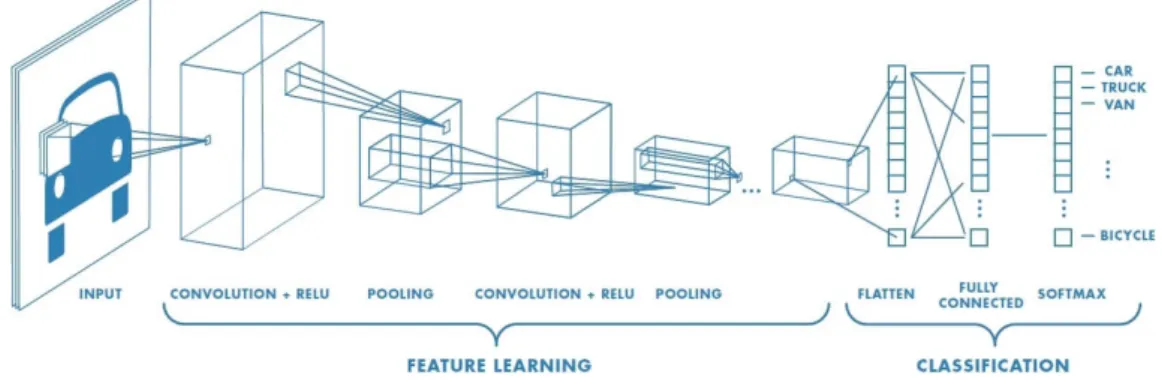
Convolutional and pooling layers account for most of a CNN’s structure and are responsible for extracting and learning relevant features from the images. At the end of the network, there are usually a few fully connected layers. In contrast to the other two kinds of layers, here every neuron of a layer is connected to all the neurons of the next layer. These are responsible for the CNN’s reasoning and producing the final output, or prediction. One of these layers converts the bidimensional feature map (extracted from the image by the previous layers) to a unidimensional vector which can then be mapped to a set of categories for classification, or serve for further processing. Figure3.1shows an example of the structure of a CNN.

Figure 3.1: Typical structure of a CNN1

The way each layer transforms its input to its output is dependent on a number of parameters, commonly called weights. As with any machine learning algorithm, CNNs need to be trained with labeled data, and in particularly high amounts. The training of a CNN consists of an interative process where, after running each image through all the layers, the weights are adjusted in an attempt to match the prediction with the expected outcome (the labels). To evaluate the quality of the predictions, CNNs use a loss function to compare them with the labels. On an untrained model, the initial weights are usually random, so it is expected that the results of the first iterations are not good. However, it is expected that the loss values progressively decrease, describing an exponential decay curve, as the weights become more properly tuned. Eventually, they should converge to a (preferably low) value, meaning that it’s no longer improving and the learning process should stop [CWMG18].

Background

3.2

Transfer Learning

The requirement for large amounts of training data is one of the main disadvantages of convolutional neural networks, and the reason why they are not a viable solution in many cases. There is, however, a strategy to help circumvent this issue, called transfer learning. This consists of, instead of training models from scratch, starting with a pre-trained model [PY10]. Some popular models, created and trained during machine learning competitions, are publicly available. Most were trained on the ImageNet dataset. Transfer learning not only makes the training process faster and less resource-hungry, it also helps achieving good results with smaller datasets. While training, some layers of the CNN can be frozen, which stops it’s weights from being adjusted. Alternatively, they can be left unfrozen and, thus, the weights will be adjusted. This is commonly known as fine tuning [SRG+16].

3.3

Deep Learning with Synthetic Data

Another workaround for the lack of large amounts of data, with which positive results have previously been demonstrated, is synthetic data generation. If using artificially generated images, dataset size should no longer be a problem. This, of course, is not the ideal approach and bring its own set of problems. Specifically, it might be tough to get the CNNs to generalize from what is learned on synthetic data to real data, which is the ultimate goal. The data generation algorithm must produce realistic samples that closely resemble reality in order to make this possible. Ekbatani et. al demonstrated a successful application of this strategy in a problem of counting the number of pedestrians in street photos [KEPS].

3.4

Supporting Frameworks and Software

This section provides an overview on some frameworks and software relevant for the solution being proposed.

3.4.1 MakeHuman

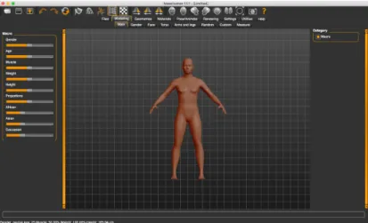
MakeHuman2is a free open-source 3D computing software designed for creating and prototyping realistic humanoid characters. The current version is developed in Python using OpenGL and the Qt framework, which enables it to run on all main operating systems. It has a very simple GUI, where most of the configurable parameters of the 3D models, such as height, weight, muscle volume, etc., are managed through sliders. This program is often used for producing virtual human characters for 3D games or animated motion pictures. It has a plugin-based architecture, but a lot of assets are built-in. Figure3.2shows a preview of its main interface.

2_{http://www.makehumancommunity.org}

Background

Figure 3.2: MakeHuman’s main interface

Nowadays it is a stand-alone application, but the project started of as a plugin for Blender (which is reviewed next), until it eventually grew too large to maintain with that architecture. During that period, it was awarded the Suzanne Award for the best Blender Python script in 2004.

3.4.2 Blender

Blender3is another open-source 3D software. However, unlinke MakeHuman, which is focused on the creation of 3D characters, Blender provides all the necessary tools to create animated films, visual effects, 3D applications and even video games, since it features an intergrated game engine. It’s been one of the state-of-the-art tools in 3D computing for several years. Instead of dealing with a single 3D object or model, in Blender the user is able to control the entire scene, with as many objects as desired, light sources, cameras, etc. Just like MakeHuman, Blender also has a modular architecture. With the appropriate plugin, it is possible to import 3D models created with MakeHuman, in order to pose or animate them.

Figure 3.3: Blender’s main interface

Background

Blender is a professional tool of great complexity, providing an enormous set of features. Hence, it also has a relatively steep learning curve associated with it, as the large amout of panels and options available can be overwhelming for unexperienced users. Figure3.3shows the initial interface of Blender’s current version.

3.4.3 Keras

Keras4is a Python open-source library developed for simplifying the use of deep learning. The creators describe it as a high-level neural network API, which runs on top of one of three other deep learning libraries: TensorFlow, CNTK or Theano. Keras makes it very simple and fast to set up and train neural networks, both recurrent and convolutional, and supports running from a GPU, which really boots performance when it comes to deep learning tasks. Besides providing a simple API for the user to create his own models, it also bundles some popular models, which can be loaded pre-trained, which really facilitates the use of transfer learning.

3.4.4 CoreML

CoreML5is a machine learning framework introduced by Apple, Inc. in 2017 with the release of the 11th version of the iOS mobile operating system. It allows the integration of previously trained machine learning models on mobile applications. This framework is the basis for other domain-specific frameworks, such as Metal Performance Shaders, which includes support for deep learning and convolutional neural networks, taking advantage of the processing power of the device’s integrated GPU.

3.5

Conclusion

This chapter briefly presented an approach to perform image recognition, one of the main computer vision problems, based on deep learning. It also reviewed a strategy to circumvent the lack of an abundant dataset, required by CNNs, which consists in the generation of artificial training data using 3D modeling software. Additionally, it reviews avaliable frameworks upon which the new solution is built. The following chapter provides a detailed description of the problem being targeted and summarizes both the proposed solution and the evaluation procedures.

4_{https://keras.io}

5_{https://developer.apple.com/documentation/coreml}

Chapter 4

Problem Statement

This chapter describes the planned approach for developing a low-cost smartphone-based solution to the presented problem. It starts with a summary of the goals and requirements, followed by an overview of the proposed solution, focusing on the main tasks, challenges and possible strategies to overcome them, taking advantage of the concepts and technologies reviewed in the previous chapter. It also presents a comparison with the existing solutions mentioned in chapter2, explaining the advantages of the one being proposed. Moreover, it describes how the new solution will be evaluated and validated.

4.1

Requirements

According to the context and problem described in chapter1, and as previously stated, the ultimate goal of this dissertation is the creation of a low-cost smartphone-based solution. Specifically, we aim to develop a mobile application that aids physiatrists and physical therapists during the usually long rehabilitation process that follows a knee injury, allowing them to estimate knee range of motion with nothing more than a smartphone.

Using the app should be simple: after selecting the desired type of measurement, the examiner will just have to point the device’s camera at the patient, immediately having the results presented on the screen. Unlike the existing photography-based solutions reviewed in chapter2, this approach

Problem Statement

should not require photographs or videos to be captured. Instead, the calculations shall be executed in real-time.

4.2

Solution Proposal

Considering the requirements explained above, the first and biggest challenge is performing accurate image recognition. The system must be able to detect when the camera is pointing at a human leg, recognizing the shape and retrieving the desired information, which are the coordinates of three key points in the image (the knee, the center of the thigh and the center of the lower leg) required for the calculation of the joint’s angle.

Existing literature describes multiple techniques for performing computerized image recog-nition. In this dissertation, we decided to explore an approach based on deep learning using convolutional neural networks. The usage of this machine learning technique for image recognition is increasing fast, as research has been revealing surprisingly positive results. Recently, this has become a very common approach in medical image analysis [LKB+17]. However, large datasets are required to adequately train convolutional neural networks. Since there is no suitable dataset available, we will synthesize one, taking advantage of 3D modeling software reviewed earlier. As a final step, the solution should be implemented as a smartphone application, taking advantage of Apple’s CoreML framework, reviewed in chapter3.

4.3

Evaluation

Since the neural networks will be trained using synthetic data, the main goal is two fold: (i) to achieve high accuracy in synthetic images, and (ii) to accurately transfer/generalize these capabilities for real images. A non-artificial validation set will be created after capturing images of the leg, simulating a treatment environment, and manually labeling them by marking the expected coordinates to be compared with the neural network’s predictions. At a more advanced stage, once the proposed solution is implemented and a functional mobile application is developed and ready to be used, it should be tested by actual physical therapists and physiatrists from a few local clinics, with the collaboration of Fábio Rocha, a physical therapist working as an external advisor in this dissertation. During the course of multiple therapy sessions with patients recovering from knee injuries, range of motion shall be measured using both the proposed solution and the traditional methods for comparison.

4.4

Conclusion

As explained in the previous sections, this novel solution has some key advantage points when compared to state of the art alternatives, especially in terms of usability. The strategy relies on recent developments in the field of image recognition, where the use of deep learning has been showing

Problem Statement

impressively positive results. The upcoming chapter is the first one covering the implementation details of this project, starting with synthetic data generation.

Problem Statement

Chapter 5

Synthetic Dataset Generation

5.1 3D Model Creation . . . 21 5.2 Manipulation and Posing . . . 22 5.3 Automated Data Generation . . . 23 5.4 Conclusion . . . 25

This chapter focuses on the generation of the synthetic image dataset with which the convolutional neural networks were trained. As previously stated, a 3D model of the human body was used in order to generate large amounts of realistic, anatomically accurate and varied image samples, as required by the deep learning technique that was applied.

5.1

3D Model Creation

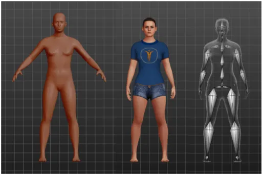
The first step of the data synthesis process was obtaining a 3D model of the human body. This was achieved using the open-source software MakeHuman1, a tool developed for the creation of three-dimensional characters. The program initially presents the user with a basic humanoid model, which was then manipulated to more accurately resemble an actual human being, since MakeHuman allows the user to tweak a large set of parameters regarding the shape and volume of body parts, textures, materials and even clothing. Not only does this model have a realistic human body shape, but it is also rigged, meaning the 3D mesh is bound to a digital skeleton consisting of bones and joints, which makes it possible to pose the character according to the requirements. Figure5.1shows both the initial and final characters, as well as the corresponding skeleton. This software, however, offers very limited options in terms of posing, only allowing the user to choose

Synthetic Dataset Generation

from a small set of predefined poses. Since the goal is to synthesize images similar to those a physical therapist would capture with the smartphone in order to measure the knee’s flexion angle, it is essential to manipulate the position of the character’s legs, especially the knee joints. This was achieved with a different software, as explained in the next section.

Figure 5.1: MakeHuman 3D models

5.2

Manipulation and Posing

In order to manipulate the 3D model created with MakeHuman, it was imported to another open-source software, Blender2, via the MHX2 format. This program provides all the necessary features to set up an appropriate scene for generating the image samples. It allows the user to select and manipulate individual bones of the character’s skeleton. Different angles of flexion were easily applied to the knee by simply rotating the lower leg bone. However, applying this single transformation generated, in many cases, unrealistic poses. When a patient is lying on their back on a treatment table, flexing the knee also requires a flexion of the hip. Thus, a 1:2 relation between the hip’s and the knee’s flexion angles was defined, ensuring the heel was permanently aligned with the torso, as if it was resting on the treatment table, as seen in figure5.2.

At this point, an image resolution of 200x150 pixels was established3, and the scene’s camera in Blender was configured accordingly. One important concern was making sure that the entire leg was captured by the camera, regardless of the angle of flexion. This was achieved using Constraints, a Blender feature that allows an object’s properties to be controlled using variables (such as the properties of a different object). Specifically, an invisible object, consisting of a single point in space, was inserted into the scene to serve as the target of the camera, which is always pointing in

2_{https://www.blender.org/}

3_{This decision is explained in §6.3(p.30)}

Synthetic Dataset Generation

Figure 5.2: Different knee flexion angles in Blender

its direction from a perpendicular perspective, according to its constraints. This point’s position is also controlled by constraints: it permanently matches the centroid of the triangle described by the knee, the hip and the ankle. This approach, combined with an appropriate distance of the camera, guarantees that the leg is always centered and fully captured.

Besides the camera and the character, the 3D scene also contains one light source positioned above the model to create appropriate lightning conditions. Additionally, in order to obtain more diverse data, multiple different-toned skin textures included with the MakeHuman software were used. Some examples are presented in figure5.3.

Figure 5.3: Examples of different skin textures used

5.3

Automated Data Generation

Having the scene set up, the dataset generation task was automated by taking advantage of Blender’s Python API. A simple script was developed to repeatedly render images from the scene’s camera, while randomly applying different flexion angles between each iteration. For every rendered image, the program also writes to a comma-separated values (CSV) file the coordinates of the three points of the leg necessary for determining the flexion angle: the centers of the thigh, the knee and the lower leg. Blender’s API provides methods to retrieve the bi-dimensional position of an object in the camera’s frame. The returned values are normalized, in the interval [0,1], and the origin corresponds to the image’s bottom-left corner. However, writing to the file, they are converted to absolute pixel values, by multiplying each coordinate by the corresponding image dimension

Synthetic Dataset Generation

(200x150 pixels), and also transposed to a coordinate system where the origin is the top-left corner of the image, as commonly observed in computer graphics.

x0= 200x y0= 150(1 − y)

(5.1)

In order to match each image with its set of coordinates, its filename, which is a numerical index (excluding extension), is also stored in the CSV file. Thus, the data is structured as shown in table5.1:

Table 5.1: Example of data stored in the CSV file img thigh_x thigh_y knee_x knee_y leg_x leg_y

0 62 74 98 71 137 73

1 64 69 98 61 132 73

2 85 62 99 30 114 64

3 70 67 98 45 129 67

... ... ... ... ... ... ...

At the top of the Python script, some parameters can be adjusted in order to configure the data generation process. These include the number of samples to be generated, the range of possible knee flexion angles and also a maximum rotation offset, relative to the patients leg, for the camera’s position. This offset is used because, in a real-case scenario, it is virtually impossible for the therapist to set the camera in an exact perpendicular direction to the plane defined by the patient’s leg. Thus, at each iteration, not only a random flexion angle is computed, but also a rotation for the camera. This rotational range should, however, be small, as significant rotations cause perspective distortion, making it impossible to accurately measure the real angle in the image.

Figure 5.4: Examples of synthesized data

Synthetic Dataset Generation

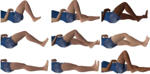
Figure5.4shows different types of samples that were obtained using this script: in the first column, only the front leg is visible (an attempt to simplify the deep learning process); in the middle one, both legs are visible. However, while the front leg is posed with random flexion angles, the other leg is straight in a resting position. And in the last column, also both legs are visible, but a different skin texture is randomly chosen for each sample. All images have a fully transparent background and were exported in Portable Network Graphic (PNG) format.

5.4

Conclusion

The presented process constitues an easy method of obtaining large amounts of data for training the neural networks. However, the size of the dataset is not the only relevant aspect. While the images look considerably realistic, they are all very similar: the only variations are the flexion angle, the camera angle and the skin tone. The next chapter explains additional approaches to improve the quality of these datasets in terms of diversity.

Synthetic Dataset Generation

Chapter 6

Image Recognition

6.1 Supporting Libraries and Resources . . . 27 6.2 Image Augmentation . . . 28 6.3 CNN Architectures . . . 30 6.4 Training . . . 33 6.5 Conclusion . . . 43

After going through the challenge of obtaining a suitable amount of data for the solution being presented, the following sections review the actual process of attempting to build a convolutional neural network that is capable of recognizing the three relevant coordinates mentioned earlier in real images, which ultimately allows the calculation of the knee’s flexion angle.

6.1

Supporting Libraries and Resources

This part of the project was implemented using the Python 3.6 programming language, along with some useful frameworks and libraries. The core of this solution is built using Keras 2.2.0, a popular deep learning Python library, running on top of Google’s TensorFlow 1.8.0. This stack provides simple and straightforward prototyping of convolutional neural networks, which greatly simplified the process of testing multiple different approaches. While it’s API allows the user to create custom CNN models, the framework has avaliable implementantions of a few popular architectures, such as MobileNet, DenseNet, VGG16 and InceptionV3, among others. Additionally, it is possible to load these models with weights pre-trained on ImageNet, a massive image dataset commonly used in visual object recognition research. The following sections explain how these features were used in the development of the solution. The management and manipulations of images and data structures

Image Recognition

was supported by NumPy and Pillow, two Python libraries widely used in scientific computing. All training tasks were executed on a dedicated nVidia GeForce GTX 1080 Graphics Processing Unit.

6.2

Image Augmentation

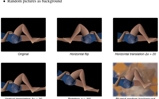
As stated earlier, synthesizing a dataset has the advantage of easily obtaining a large number of samples. However, introducing enough diversity to enable the neural networks to generalize what is learned from this data to real-life examples is a challenge. Adding to the strategies used during the generation step (flexion angle, camera position and skin texture), some image augmentation techniques were applied during the training process, which is commonly referred to as online augmentation. These are:

• Horizontal flipping, with probability of 50%

• Random horizontal translations, with ∆x ∈ [−20, 20] • Random vertical translations, with ∆y ∈ [−10, 30] • Random rotations, with α ∈ [−30◦, 30◦]

• Random pictures as background

Figure 6.1: Examples of the transformations applied to the dataset

For each image that was loaded from the dataset for training, any of these transformations would be randomly applied and the labels updated accordingly. Multiple tests have been executed, with different combinations of transformations being applied, and also with variable ranges of values for

Image Recognition

the translations and rotations. Figure6.1shows the results of applying these transformations to a sample of the dataset.

While all techniques aim at improving the quality and diversity of the dataset, each has a specific theoretical goal. While the original dataset only contains images of the right leg of the character, applying horizontal flips should help the network learn how to recognize images of both legs. Rotating should, for instance, improve the results in images where the patient is not lying down on the treatment table or the camera is not properly leveled. Translations should help the network generalize for cases where the leg is not exactly centered in the image.

Horizontal flips are a type transformation that requires special attention, since it changes the order of the labeled points. The original order is first the thigh, then the knee and lastly the lower leg. For the neural networks, however, this order has no meaning and we could easily encounter a situation where the results are terrible, even though the network did perform good predictions... but in the wrong order. For instance, if the expected output was [(1, 0), (0, 0), (−1, 0)] and the network predicted [(−1, 0), (0, 0), (1, 0)], the calculated loss would be 2, when it should actually be 0, since the three points match perfectly. Thus, it is important that the networks are trained to always predict in the same order. In all other samples, with the rest of the transformations, the labels are ordered from left to right (x values are in increasing order). This problem has a simple solution: when a horizontal flip is applied, the labels of the first and third points are swapped. This way we ensure the labels are always ordered from left to right, maintaining a pattern which will help during the training process.

Figure 6.2: Some of the photographs used as background

One of the aspects that make all the training samples so similar is the background. All images were generated with a transparent background, having 4 channels: red, green, blue and alpha (RGBA image). However, before they can be used for training, they must be converted to have only 3 channels: red, green and blue (RGB images). The Pillow library provides a method for this conversion, which by default sets the previously transparent pixels to full black. If a network is trained using these images, the performance on real images where the background is not uniform

Image Recognition

and black will certainly be poor. The network should be able to recognize which image pixels correspond to the patient’s leg and disregard the rest, as they have no meaning. Hence the last transformation mentioned — background change. To circumvent this issue, each time an image is loaded for training, it is pasted over a random photograph before the RGBA to RGB conversion. These photographs were provided by [JDS08], a dataset with 1491 personal holidays photos. Figure6.2shows some of these images.

This is the first technique to be applied, so, the background is also affected by all the following transformations. Before merging them with the leg samples, a gaussian blur filter with a 2px radius is applied to reduce the amount of detail of the pictures and making them smoother.

Again, multiple tests were executed in order to assess the impact of these transformations. We started by applying none, and progressively enabling them, one by one, while also experimenting with different combinations. While this should, in theory, improve the results, that’s not necessarily the case, as the results will demonstrate.

6.3

CNN Architectures

During the execution phase of this project, different CNN architectures were tested and compared, in an attempt to achieve the best results. Given the characteristics of the available dataset, it was decided to start by using transfer learning instead of training a network from scratch. That process was simplified by the Keras framework, which bundles some popular CNN models pretrained with the ImageNet dataset. Two of those were selected: InceptionV3[SVI+] and VGG16[SZ14]. A third, custom model, was also used. This is a much simpler model that the other two, and it was trained from scratch on the synthetic dataset. This custom model will be referred to as Eva.

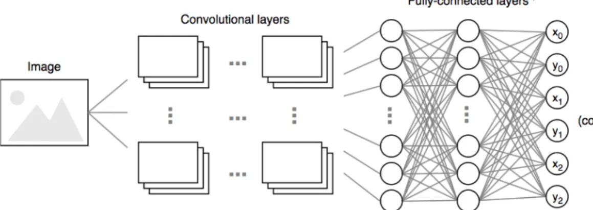
While the Eva model was designed for this particular situation, InceptionV3 and VGG16 had to be slightly modified in order to be used — specifically, the first and last layers. The first layer because they were trained on images with a different resolution than those in our dataset, which are 200x150 pixels. This resolution was decided taking into account the minimum size accepted by common CNN models such as the ones being used. For instance, while the minimum size suitable for VGG16 is 48x48 pixels, InceptionV3 requires, at least, 139x139 pixels. The chosen resolution should be large enough to be used with any model, while being, at the same time, small enough not to significantly slow down the training process. Thankfully, Keras is prepared for this situation, and allows the user to specify a custom input shape when loading pre-trained models. And also the last layer, since both VGG16 and InceptionV3 were designed for the ImageNet classification problem, which has 1000 distinct classes of images. Thus, both have a final layer with exactly 1000 neurons, which is innapropriate for the problem being solved here. Our problem is different in two aspects: first, instead of predictions on 1000 classes, we need only 6 predictions (the x and y coordinates for the centers of the thigh, knee and lower leg); second, this is a regression task, not classification. In order to match these requirements, the last layer must have exactly 6 neurons and no activation function, so the network outputs the untrasformed numerical values. Figure6.3represents this structure.

Image Recognition

Figure 6.3: Diagram representing the required CNN structure

When a Keras model is created or modified, it must then be compiled before being used. During this step, the user must specify a loss function and an optimizer to run during the training process. With all three models tested, the chosen optimizer was RMSProp[WMH+17], which comes bundled in Keras. As for the loss, a custom function was implementing for calculating the total euclidean distance between predicted (x0i, y0i) and the expected (xi, yi) three points, according to (6.1).

` = 2

∑

As explained earlier, after loading the InceptionV3 model with pre-trained weights, the final layer was changed in order to fit the current problem. Table6.1shows the last fully-connected layers after this change.

Table 6.1: InceptionV3 final fully-connected layers (modified) Layer Type Neurons Parameters

... ... ...

GlobalAveragePooling2D 2048 0

Dense 1024 2098176

Dense 6 6150

Since it was decided to use transfer learning in order to both get improved results and reduce training time, at first, only the last three fully-connected layers were set as trainable. This means only the weights of these layers will be fine-tuned for the synthetic dataset. Thus, here’s the summary of the network’s parameters:

• Total parameters: 23,907,110 • Trainable parameters: 2,104,326 • Non-trainable parameters: 21,802,784

Image Recognition

As shown here, most of InceptionV3’s parameters are on the convolutional layers, leaving only a small amount of parameters to be trained (roughly 9%). So, instead of training only the fully connected layers, this time the last 60 layers were set as trainable. This raised the percentage of trainable parameters to nearly 45%:

• Total parameters: 23,907,110 • Trainable parameters: 10,605,510 • Non-trainable parameters: 13,301,600

6.3.2 VGG16

A similar process was used for the VGG16 model. Table6.2shows the fully-connected layers after it was adapted to the problem:

Table 6.2: VGG16 final fully-connected layers (modified) Layer Type Neurons Parameters

... ... ...

Flatten 12288 0

Dense 4096 50335744 Dense 4096 16781312

Dense 6 24582

The convolutional layers on this model were equally frozen. However, a significant difference from InceptionV3 is evident when it comes to the trainable parameters:

• Total parameters: 81,856,326 • Trainable parameters: 67,141,638 • Non-trainable parameters: 14,714,688

Unlike the previous model, the majority of VGG16’s parameters are on the fully-connected layers. In this model, about 82% of the parameters are trainable. However, when using Transfer Learning, it is advisable to set all fully-connected layers as trainable, since they act as the classifier or, in this case, as the regressor, and are quite specific to the data domain.

6.3.3 Eva

Eva was the name given to the model that was created from scratch. It is much smaller and simpler in comparison to InceptionV3 and VGG16, having only 3 convolutional layers and a total of 11. Code block6.1shows the Python script responsible for the creation of this model, using built-in Keras’ methods:

Image Recognition

1 Eva = Sequential([

2 Conv2D( filters=32,kernel_size=(3,3), activation="relu", input_shape=(150,200,3) ), 3 MaxPooling2D( pool_size=(2,2), strides=(2,2) ),

4 Conv2D( filters=64,kernel_size=(4,4), activation="relu" ), 5 MaxPooling2D( pool_size=(2,2) ),

6 Conv2D( filters=4, kernel_size=(3,3), activation="relu" ), 7 MaxPooling2D( pool_size=(2,2) ),

8 Flatten( ),

9 Dropout( rate=0.2 ),

10 Dense( units=100, activation="relu" ), 11 Dense( units=50, activation="relu" ), 12 Dense( units=6 )

13 ])

Code Block 6.1: The script for generating the Eva model

As can be seen on table6.3, this produces a simpler and less deep model, with a much smaller set of parameters.

Table 6.3: Layers of the Eva CNN model Layer Type Output Shape Parameters Conv2D (None, 148, 198, 32) 896 MaxPooling2D (None, 74, 99, 32) 0 Conv2D (None, 71, 96, 64) 32832 MaxPooling2D (None, 35, 48, 64) 0 Conv2D (None, 33, 46, 4) 2308 MaxPooling2D (None, 16, 23, 4) 0 Flatten (None, 1472) 0 Dropout (None, 1472) 0 Dense (None, 100) 147300 Dense (None, 50) 5050 Dense (None, 6) 306

However, this model is not pre-trained on any dataset. Thus, all layers must be trained, since weights are randomly initialized. Even so, given the total number of parameters, training this model will be quite less time-consuming than the other two.

• Total params: 188,692 • Trainable params: 188,692 • Non-trainable params: 0

6.4

Training

In this phase of the project, the three CNN models will be tested with different combinations of image augmentation techniques applied to the dataset. The training set has 3000 samples and is the same in all tests (only differs by the transformations applied on the fly). The validation set, however, will not be exactly the same in each experiment. It will always be composed of a total

Image Recognition

of 500 samples: 25 synthetic images with the original skin texture and only one leg visible; 425 synthetic images with varied skin textures and both legs visible; and 50 real pictures (originally only 3, to which similar image augmentation was applied in advance). The only difference between the validation sets of each experiment is, again, the augmentation techniques applied. For each different combination in an experiment, a matching validation se, with the same transformations applied is used. Figure6.4shows some samples from the validation set.

Figure 6.4: Samples from the validation sets

In each of the experiments, the learning curves of the loss values (both on training and validation sets) are presented. The Eva model is represented by theorangeline, InceptionV3 by theblueand VGG16 by thedark redone. Along with these curves, a few sample predictions executed by these models are shown, providing a more visual outcome. Lastly, the minimum loss values reached by each model are also documented.

Image Recognition

6.4.1 Test #1: No augmentation

The first test consisted of training on the original dataset, without performing any image augmenta-tion procedures.

Figure 6.5: Training curves for Test #1. The left and right charts correspond to the training and validation sets, respectively.

Figure 6.6: Sample predictions after Test #1

The Eva model reached a minimum loss of 12.24 in the testing set and 7.318 in the validation set. The Inception V3 model reached a minimum loss of 8.023 in the testing set and 12.37 in the validation set. The VGG16 model reached a minimum loss of 13.60 in the testing set and 26.94 in the validation set.

Image Recognition

6.4.2 Test #2: Horizontal flips

In the second test, dataset images are horizontally flipped with a probability of 50%.

Figure 6.7: Training curves for Test #2. The left and right charts correspond to the training and validation sets, respectively.

Figure 6.8: Sample predictions after Test #2

The Eva model reached a minimum loss of 13.61 in the testing set and 11.05 in the validation set. The Inception V3 model reached a minimum loss of 7.790 in the testing set and 18.49 in the validation set. The VGG16 model reached a minimum loss of 13.90 in the testing set and 21.60 in the validation set.

Image Recognition

6.4.3 Test #3: Translations

On the third test, dataset images are horizontally translated a random value of the range [-20,20] and vertically translated a random value of the range [-10,30].

Figure 6.9: Training curves for Test #3. The left and right charts correspond to the training and validation sets, respectively.

Figure 6.10: Sample predictions after Test #3

The Eva model reached a minimum loss of 15.25 in the testing set and 10.54 in the validation set. The Inception V3 model reached a minimum loss of 8.236 in the testing set and 19.57 in the validation set. The VGG16 model reached a minimum loss of 13.90 in the testing set and 18.70 in the validation set.

Image Recognition

6.4.4 Test #4: Background images

On the fourth test, a random background selected from the previously mentioned dataset is added to each training sample.

Figure 6.11: Training curves for Test #4. The left and right charts correspond to the training and validation sets, respectively.

Figure 6.12: Sample predictions after Test #4

The Eva model reached a minimum loss of 11.97 in the testing set and 13.67 in the validation set. The Inception V3 model reached a minimum loss of 6.983 in the testing set and 14.36 in the validation set. The VGG16 model reached a minimum loss of 11.43 in the testing set and 25.69 in the validation set.

Image Recognition

6.4.5 Test #5: Rotations

On the fifth test, rotations are applied to the dataset samples, relative to their center, of random amplitude in the range [-15◦,15◦]

Figure 6.13: Training curves for Test #5. The left and right charts correspond to the training and validation sets, respectively.

Figure 6.14: Sample predictions after Test #5

The Eva model reached a minimum loss of 10.50 in the testing set and 17.15 in the validation set. The Inception V3 model reached a minimum loss of 6.609 in the testing set and 21.37 in the validation set. The VGG16 model reached a minimum loss of 13.69 in the testing set and 47.42 in the validation set.

Image Recognition

6.4.6 Test #6: Flips and translations

On the sixth test, both horizontal flips and translations are applied.

Figure 6.15: Training curves for Test #6. The left and right charts correspond to the training and validation sets, respectively.

Figure 6.16: Sample predictions after Test #6

The Eva model reached a minimum loss of 15.08 in the testing set and 12.36 in the validation set. The Inception V3 model reached a minimum loss of 8.314 in the testing set and 15.24 in the validation set. The VGG16 model reached a minimum loss of 15.23 in the testing set and 21.94 in the validation set.

Image Recognition

6.4.7 Test #7: Flips, translations and rotations

On the seventh test, samples get randomly flipped, translated and also rotated.

Figure 6.17: Training curves for Test #7. The left and right charts correspond to the training and validation sets, respectively.

Figure 6.18: Sample predictions after Test #7

The Eva model reached a minimum loss of 14.98 in the testing set and 17.16 in the validation set. The Inception V3 model reached a minimum loss of 8.384 in the testing set and 22.10 in the validation set. The VGG16 model reached a minimum loss of 14.07 in the testing set and 28.12 in the validation set.

Image Recognition

6.4.8 Test #8: Flips, translations, rotations and backgrounds

Lastly, on the eighth test, all four image augmentation techniques are used simultaneously.

Figure 6.19: Training curves for Test #8. The left and right charts correspond to the training and validation sets, respectively.

Figure 6.20: Sample predictions after Test #8

The Eva model reached a minimum loss of 15.53 in the testing set and 19.89 in the validation set. The Inception V3 model reached a minimum loss of 8.320 in the testing set and 22.64 in the validation set. The VGG16 model reached a minimum loss of 13.97 in the testing set and 32.22 in the validation set.

Image Recognition

6.5

Conclusion

As we can observe in table6.4, regardless of the image augmentation techniques used, InceptionV3 always achieves the best loss values in the training set, while Eva achieves the best results in the validation set. Hence, although the smoothed training lines presented in the previous section might cause a different impression, we can conclude that Eva seems to generalize better to unseen images. However, both these models achieved similarly good results. On the other hand, VGG16 results fell short to the expectations. In some test cases, the training curve did not even converge properly and the predictions hit significantly off target, evidencing difficulty in generalizing to real data. Table 6.4: Results of the 8 test scenarios. T and V columns represent the minimum loss values on the training and validation sets, respectively. Lower results are better.

Test I3 T I3 V VGG T VGG V Eva T Eva V #1 8.02 12.37 13.60 26.94 12.24 7.32 #2 7.79 18.49 13.90 21.60 13.61 11.05 #3 8.24 19.57 13.90 18.70 15.25 10.54 #4 6.98 14.36 11.43 25.69 11.97 13.67 #5 6.61 21.37 13.69 47.42 10.50 17.15 #6 8.31 15.24 15.23 21.94 15.08 12.36 #7 8.38 22.10 14.07 28.12 14.98 17.16 #8 8.32 22.64 13.97 32.22 15.53 19.89

Figure 6.21: InceptionV3 predictions on edited photographs (background removed)

Image Recognition

While there is certainly much room for further improvement, specifically in terms of the diversity of the synthetically generated dataset, this outcome indicates that some good progress has been made. Figures6.21and6.22are evidence that, while the background on real photographs does interfere with the network’s behavior, it seems to work around that fairly well.

While there might be many reasons for that, the fact that InceptionV3, which was pre-trained on ImageNet, achieved a good performance offers some significant indication of the positive impact transfer learning can have. The final results are also aligned with previous research indicating synthetic data generation as a valid alternative for training convolutional neural networks when an appropriate dataset is unavailable.