Vol.57, n.2: pp. 274-283, March-April 2014
ISSN 1516-8913 Printed in Brazil BRAZILIAN ARCHIVES OF
BIOLOGY AND TECHNOLOGY
A N I N T E R N A T I O N A L J O U R N A L
Generation of Intensity Duration Frequency Curves and
Intensity Temporal Variability Pattern of Intense Rainfall
for Lages/SC
Célio Orli Cardoso
1*, Idelgardis Bertol
2, Olívio José Soccol
1and Carlos Augusto de Paiva
Sampaio
11Departamento de Agronomia; Universidade do Estado de Santa Catarina; Lages - SC - Brasil. 2Departamento de
Solos e Recursos Naturais; Universidade do Estado de Santa Catarina; Lages - SC - Brasil
ABSTRACT
The objective of this work was to analyze the frequency distribution and intensity temporal variability of intense rainfall for Lages/SC from diary pluviograph data. Data on annual series of maximum rainfalls from rain gauges of the CAV-UDESC Weather Station in Lages/SC were used from 2000 to 2009. Gumbel statistic distribution was applied in order to obtain the rainfall height and intensity in the following return periods: 2, 5, 10, 15 and 20 years. Results showed intensity-duration-frequency curves (I-D-F) for those return periods, as well as I-D-F equations:
89 , 0 20
,
0 .( 30)
.
2050 + −
= Tr t
i , where i was the intensity, Tr was the rainfall return periods and t was the rainfall duration. For the intensity of temporal variability pattern along of the rainfall duration time, the convective, or advanced pattern was the predominant, with larger precipitate rainfalls in the first half of the duration. The same pattern presented larger occurrences in the spring and summer stations.
Key words: maximum rainfall, I-D-F curves, Gumbel distribution, intensity rainfall
*Author for correspondence: a2coc@cav.udesc.br
INTRODUCTION
Knowledge on intense rainfall characteristics is highly valued in Engineering and Agronomy for the dams dimensioning and hydraulic projects for irrigation, drainage and the control of water erosion, as well as facilitating the understanding of hydrological processes of river basins. Hence, it is desirable to know the magnitude and frequency of intense rainfall characterized by its duration, intensity and return period, using among other techniques, the probability principles. According to Pruski et al. (2002), the knowledge of the intense rainfall characteristics is scarce in most Brazilian's regions, and even at regions with satisfactory rainfall recording rain gauges, the
Parameters for equation of intense rainfall are obtained by a non-linear regression based on pluviograph data. According to Costa and Brito (1999) and Silva et al. (1999), the determination of intense rainfall equation shows greater difficulties due to the scarcity of rainfall records; significant barriers to obtain them, low density of rainfall pluviograph data, and the small observation period to get them. Furthermore, the methodology used to achieve the rainfall records demands an exhaustive work of data tabulation, analysis and interpretation of a large quantity of pluviograph data. For this reason, few studies in Brazil have been developed on this subject. In Brazil, according to Silva et al. (1999), rainfall recording rain gauges are more restrictive than pluviometric ones, because most of the recordings are still on the shelves of the office in charge, waiting for someone to scan the pluviograph records. Hence, some methodologies were developed in order to get rainfalls intensity from the pluviometric data, by scanning the pluviograph records and, to some extent, solving the matter highlighted before. Those methodologies apply the coefficients to transform “one day” (or 24 h) rainfalls in shorter duration rainfalls. Among those methodologies, one is the disaggregation of “one day” or 24 h rainfall data by CETESB (1986).
According to Genovez and Zuffo (2000), it is important to highlight that DNOS (National department of Sanitation Works) studies made in 1957 and used by CETESB (1986) to determine the relations between 24 h rainfalls and shorter duration rainfalls. Besides being late, they were based on a reduced number of pluviographs stations. However, rainfalls from different Brazilian regions can be provoked by different mechanisms. Accordingly, those relations do not substitute recording rain gauges data, but only indicate an approximate relation among rainfall durations. Because this is a medium relation, it is much more representative when more reliable is the region where it will be applied. Thus, those relations should be determined for smaller regions with water homogeneity.
According to Genovez and Zuffo (2000), the methods that are based in the relationships among intense rainfalls of different durations have regional validity, although the medium values of these relationships are very close of several parts of the world. For the estimates at different places, it is convenient to establish new coefficients,
related to the characteristics of the climatic places. When studying intense rainfall, it does not matter to know the maximum rainfall observed in a rainfall series, but mainly to predict what kind of rainfall can occur in certain region with determined frequency (Villela and Matos 1975). By correlating the rainfall intensity and duration for a specific return period, the more intense the rainfall, the shorter its duration, showing a hyperbolic-type curve (Huff 1967). According to Linsley and Franzini (1978), this relation can be represented by two types of equation; one for the rainfalls with duration between 5 to 120 min, and another one for rainfalls with duration higher than 120 min, known as Talbot’s equations. More complex I-D-F equation can just be established by the statistical examination of long series of local rains (Santos et al. 2009), and the results cannot be extended to other regions. These results can be showed graphically as curves relating the intensity and duration and defining one curve for each return period. After a number of previous observations, hydrologists have developed an equation, which fits in well within the experimental data, named “Equation of Intense Rains”, or “Intensity-Duration-Frequency Equation”. Cardoso et al. (1998), using a daily rain disaggregation model and the method of relations proposed by CETESB (1986), from “one-day rain” data, obtained I-D-F rainfall equation for Lages/SC as follow: i=2050Tr0,17(t+29,42)−0,89, where i was the intensity (mm h-1), Tr was the
return period (year) and t was the rainfall duration
(minute). In this study, authors used duration from 5 to 120 min and more than 120 min for return periods from 2 to 100 years.
variability, which was necessary, for example, for hidrographies analysis.
Back (2001) studying the daily data of maximum rainfalls of a hundred pluviometrics stations of Santa Catarina’ State observed that the Gumbel’s distribution presented the best adjustment to the data observed in 60% of the stations and in 93% of the stations with less than twenty years of data. Silva et al. (1999) adapted a theoretical model of probability distribution to rainfall data for Rio de Janeiro and Espírito Santo states and established the I-D-F relation of the rainfalls in this cites. A similar study was made by Damé et al. (1996) for the annual rainfall and monthly maximum and minimum precipitation for some regions in Rio Grande do Sul. In another study, Robaina (1996) developed a model to estimate the rainfalls shorter than 24 h in Rio Grande do Sul, which was more appropriate when estimated rainfalls were compared to observed ones. Other works using the similar methodologies were carried in this and another Brazilian’s states to obtain the I-D-F relationships in these places. These included by Eltz et al. (1992) in Rio Grande do Sul, Fendrich (1998) at Paraná’s State, Pinto et al. (1999) in Minas Gerais, Genovez and Zuffo (2000) in São Paulo, Oliveira et al. (2000) in Goias, Silva et al. (2002) in Bahia, Silva et al. (2003) in Tocantins, Oliveira et al. (2005) in Goias and Distrito Federal, Santos et al. (2009) in Mato Grosso do Sul, Moruzzi et al. (2009) in Rio Claro, SP, Castro et al. (2011) in Cuibá, MT, and Back (2002) e Nerilo et al. (2002) to Santa Catarina’s State. Other important aspect of intense rainfalls is the intensity variation pattern during the rainfalls duration time. Sentelhas et al. (1998) analyzed and characterized the rainfall time distribution with 4-h duration for Piracicaba, SP, showing an intensity distribution model with higher occurrence probability, from October to March. In 85% of these cases, the predominant model was a negative exponential distribution, with fractions of total precipitation of 69.3% (first hour), 16.3% (second hour), 9.4% (third hour) and 5% (fourth hour), typifying an advanced, frontal, or convective rainfall distribution.
There are very few studies in Brazil involved on the characterization of rainfall intensity variation during its occurrence, while this kind of study is very common in other countries (Huff 1967, Preul and Papadakis 1973; Olsson and Berndisson 1998; Evangelista et al. 2005). According to Cruciani (1986), the knowledge of the intensity makes the
temporal distribution model of intense rainfall in a specific region more realistic for the hydrological forecast for engineering projects in the rural and urban areas. He suggested the characterization and quantification of the run-off more precisely, which was possible by the application of hidrographies analysis methods, as Shemtan’s and Soil Conservation Service ones, among others. According to Machado et al. (2008), rainfall erosivity is calculated based on its physical characteristics, and according to Evangelista et al. (2005) the temporal variation pattern of the rainfall intensity is one of the most important factors in soil erosion, and its characterization is fundamental to conservationist planning. Despite studies on erosive potential of rainfalls in several Brazilian regions (Eltz et al. 2001; Bertol et al. 2002; Moreti et al. 2003; Albuquerque et al. 2005; Evangelista et al. 2005), there are few studies on the physical aspects of rainfall as those related to rainfall intensity variation during its occurrence, that is, with rainfall intensity temporal variation patterns.
Thus, the aim of this study was to describe the representative model of temporal distribution for intense rainfall with duration from 10 min to 18 h, and their occurrence probabilities in Lages/SC and, from these, the I-D-F equation to analyze the 1) frequency distribution of maximum rainfall values from recording rain gauges observations, 2) intensity temporal conducts of intense rainfalls, 3) to get the characteristics of intense rainfalls, such as the average intensity, duration and frequency and their relations, and 4) to draw the intensity-duration-frequency curves of the observed rainfalls and the equation of intense rainfalls.
MATERIALS AND METHODS
intervals of 10 min and typed (Excel spreadsheets), according to the corresponding rainfalls heights.
Intense rainfall events were selected according to criteria established by Cruciani et al. (2002), subdivided at four equal intervals (quarters) according to their duration and arranged in histograms, selecting the more frequent patterns of temporal distribution for analyzing. For statistical analysis of intense rainfall probability and return period by Gumbel distribution, in each historical observation, the maximum height for each selected duration (10, 20, 30, 40, 50 and 60 min, 2, 4, 6, 12 and 18 h) was obtained from the diary pluviograph data tabulation, constituting an annual maximum series for each duration.
Based on these values, the following systematic procedure was made: an annual maximum series was set in descending order for each durations, calculating the statistical elements of the sample: mean (µx) and standard deviation (Sx); the observed frequencies (Fi) was calculated according to the formula by Kimbal.
The reduced variable (yi) of Gumbel’s statistical distribution was calculated by the equation:
)] y y Sx. -x ( x .[ Sx y =
yi i
σ µ µ
σ − [1]
Where: yi was the reduced variable of Gumbel’s distribution; µy was the mean and σy was the standard deviation of the reduced variable; µx was the mean; Sx was the standard deviation of the sample; and xi was the random variable (maximum annual rainfall). The expected theoretical probability (Pi) was calculated according to Gumbel, by the equation:
i -y -e i =1-e
P [2] Where: Pi was the expected probability; e was the
basis of Nepierian logarithm and yi was the Gumbel’s reduced variable. The expected return period (Tri) was calculated by:
i i
P 1 =
Tr [3] Where: Pi was the expected theoretical probability. An analytical line for estimating rainfalls heights for each durations according to the expected return period without graphics was obtained through [1]
equation: z
y y Sx. -x e w Sx
y = =
σ µ µ
σ ; having:
z) -w.(x =
yi i [4]
Isolating the random variable xi, resulted an analytical line according to the reduced variable by the equation
z w y
xi= i + [5]
Setting the reduced variable according to the return period (Tri), resulted in the equation:
)] Tr 1 -ln.[-ln(1 -= y i i [6]
So, the analytical line according to the return period showed the following rating:
z w
Tr
xi i +
− − − = )] 1 1 ln( ln[ [7]
Where xi was the random hydrologic variable, that is, the maximum rainfall height expected for a given return period; Tri was the expected return period; ln was the natural logarithm; w e z were the parameters of linear equation obtained according to the statistical elements of the sample and the reduced Gumbel’s variable. Gumbel’s distribution adherence to the annual rainfall series was verified by Kolmogorov-Sminorv Test with 5% of significance.
From the equation [7], the analytical frequency lines of the maximum rainfalls for each duration was obtained, which allowed the determination of the expected maximum rainfall heights according to return period. The values of the analytical equations parameters are shown in Table 1.
Intension-Duration relationships for the rainfall duration until 120 min were obtained by Talbot equation, in order to express the relation between intensity and duration for a determined return period as follow:
td + b
a =
i [8]
For the durations larger than 120 min, the analytical expression for curves, which adjusted to the observed data was:
d td
c =
i [9]
Where: i was the rainfall intensity for an specific
return period; t was the rainfall duration; a, b, c
and d were the adjusted local parameters to determine statistically.
curves were obtained by a general equation, which described the relation among the intensity, duration and return period. It is called as “intense rainfall equation”, or “intensity-duration-frequency equation”, shown as below:
n m
) + (b
k. =
t Tr
i [10]
Where: i was the rainfall intensity; t was the
rainfall duration; Tr was the return period; k, m, n
and b were the adjusted local parameters to determine statistically.
Table 1 - Values of “w” and “z” from analytical equations of expected rainfall heights for duration periods considered to Lages/SC (eq. [5]).
Rainfall duration
Parameter
w z
10 min 0.3119 9.84
20 min 0.2753 16.72
30 min 0.1945 21.79
40 min 0.1420 25.03
50 min 0.1266 27.01
60 min 0.1211 28.65
2 h 0.1105 30.97
4 h 0.1065 33.09
6 h 0.0912 37.72
12 h 0.0695 40.71
18 h 0.0354 6.49
The parameters of an equation that provides, for any return period, the intensity for several duration periods observed were established. Parameter "b" was obtained through the arithmetic average of coefficients “b” from the Talbot equations over the selected return periods. For determining other
parameters from the rainfall equations, a non-linear regression procedure was applied on the basis of the information extracted from pluviograph data.
To analyze the temporal variation pattern, maximum rainfall events for each 10-day period of the year were subdivided at four equal intervals (1º, 2º, 3º and 4º “quarters”) and disposed in histograms. The rainfall temporal distributions was analyzed and characterized with four equal sub-periods of variable duration, selecting the distribution models most likely to occur in each season and totaling the rainfall volume (rainfall height) for each quarter.
RESULTS AND DISCUSSION
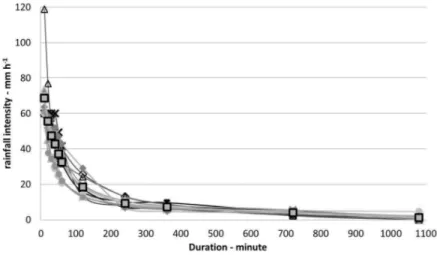
The maximum intensity of rainfall in 2002 was 118.8 mm h-1 (during 10 min), in 2003, it was 41.6 mm h-1 (for 1 h), and in 2005, it was 4.6 mm h-1 (during 18 h). In 2002, 2003, 2004 and 2009, intense rainfalls showed duration lower than 18 h (Fig. 1). With the increase of the rainfalls duration, their maximum average intensity was reduced as expected, because, according to Huff (1967), the average rainfall intensity decreased with the duration increase and, naturally, it increased with the diminution of the return period. This was because the rainfall intensity showed higher temporal variability for long-duration rainfalls, passing by low intensity and sometimes drought, which diminished the average intensity. This did not occur in short-duration rainfall, which resulted in larger average intensities of the rains.
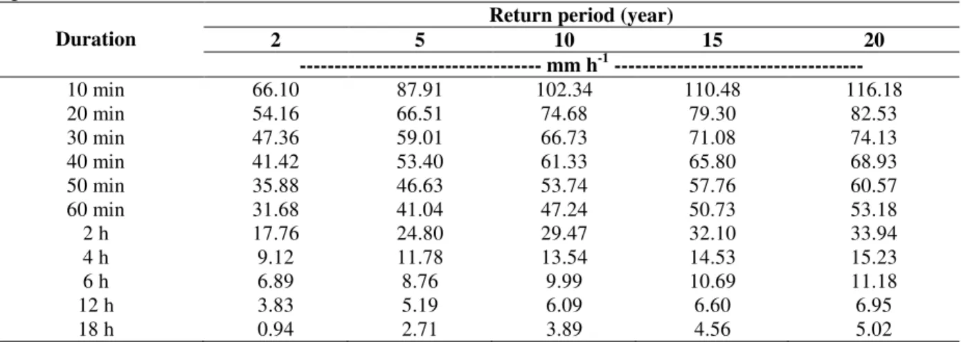
There was a gradual decrease in rainfall average intensity expected values as duration of the rainfalls increased (Table 2), in according to data obtained from other researchers (Huff 1967; Souza Pinto et al. 1973; Linsley and Franzini 1978; Righetto 1998; Pinto 1999; Soccol et al. 2010). According to Silveira (2000), it was probably due to higher intensity values, which were related to rainfall events from connective processes that by observation, passed from a condition in short-term, even in temperate climates and, sometimes, during
the winter. On the other side, lower intensity values could easily be associated to the rainfalls from the frontal processes in the displacement of air masses, which passed from a long-term scale. Intensity-duration relations allowed higher convenience and precision in obtaining maximum heights of the expected rainfalls, so facilitating the use of the rainfall data in the projects in which needed to size the hydraulic works of controlling the flow.
Table 2 - Values of rainfall average maximum intensity expected for return periods and durations selected for Lages/SC.
Duration
Return period (year)
2 5 10 15 20
--- mm h-1 ---
10 min 66.10 87.91 102.34 110.48 116.18
20 min 54.16 66.51 74.68 79.30 82.53
30 min 47.36 59.01 66.73 71.08 74.13
40 min 41.42 53.40 61.33 65.80 68.93
50 min 35.88 46.63 53.74 57.76 60.57
60 min 31.68 41.04 47.24 50.73 53.18
2 h 17.76 24.80 29.47 32.10 33.94
4 h 9.12 11.78 13.54 14.53 15.23
6 h 6.89 8.76 9.99 10.69 11.18
12 h 3.83 5.19 6.09 6.60 6.95
18 h 0.94 2.71 3.89 4.56 5.02
The values for “a” and “b” coefficients from the Intensity-Duration equations (I-D) shown in Table 3 were used in the equations for rainfall durations between 5 and 120 min (Talbot’s equation). The “c” and “d” coefficients were used in the rainfall duration equations longer than 120 min. High values of the determination coefficient showed a proper adjustment of the equations obtained from the data.
The intense rainfall equation was obtained, which
represented the Intensity-Duration-Frequency curves, predicting the average maximum intensity of the rainfalls from its duration and return period. Intense rainfall equation for Lages/SC from the analysis of diary pluviograph data was:
89 , 0 20
,
0 .( 30)
.
2050 + −
= Tr t
i [11]
where i was the intensity in mm h-1, Tr was the
return period in years and t was the rainfall
duration in min.
Table 3 - Values of the coefficients "a", "b", “c”, “d” from intensity-duration equations and from determination coefficients for the selected return periods (Tr), for Lages/SC.
Tr Duration between 5 to 120 min Duration longer than 120 min
a b r2 c d r2
2 3.179 38.09 0.82 2083 0.98 0.91
5 3.892 35.28 0.83 1014 0.81 0.88
10 4.364 34.12 0.83 834 0.75 0.89
15 4.630 33.45 0.85 779 0.72 0.88
20 4.817 33.09 0.81 751 0.71 0.87
The intense rainfall equation, or I-D-F equation obtained through the relations from the pluviograph data showed the values and shape
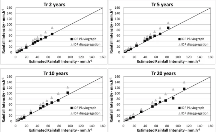
of diary rainfall and the relation proposed by CETESB (1986), whose methodologies were appropriated to estimate the short-duration rainfalls. It was observed that as the rainfalls duration increased and the gap between the estimate values increased as well in all the return periods analyzed (Fig. 2).
Therefore, a proper adjustment of the equation obtained in this study to the observed values from the pluviograph data in all the return periods was observed. Equation obtained from the pluviograph data estimated lower values than the equation obtained with the disaggregation model of one-day rainfalls from the pluviometers. Those differences were because the relations used in the disaggregation model between 24-h rainfall and lower-duration rainfalls, besides being very old, also had as basis a much reduced number of precipitation stations in Brazil as well as their bad
distribution, being quite generalized and not representing the variability and specificity of each Brazilian region. As the in different Brazilian’s regions could be provoked by different mechanisms, these relations did not replace the precipitation data registered in locu exactly, but
just indicated an approximate relationship among the precipitation durations. Thus, although they were average and generalized relations, they did not represent accurately the intense rainfall behavior in the specific region that gave better confidence in the relations obtained from the observed pluviograph data obtained in this study. Therefore, there is the need for periodic updating of those equations due to the influence of urbanization and global warming on rainfall pattern to re-evaluate and regionalizing the relationships used in disaggregation model.
Figure 2 - Observed rainfall intensity compared to the intensity estimated by IDF equation from pluviograph data (IDF pluviograph) and to the intensity estimated by IDF equation from disaggregation model (IDF disaggregation), for Lages/SC.
The I-D-F equation coefficients obtained in this work starting from the pluviograph data too were different from those obtained by Back for other cities in Santa Catarina, such as Florianópolis
characteristics of the rainfall in the respective regions. According to Genovez and Zuffo (2000), a possible physical explanation for this could also probably be the dimensions and properties of the common mechanisms of convective rainfall, responsible for the high intensity and short duration of heavy rains in different parts of the world. Thus, one should not ignore the differences that regional rainfall featured due to local characteristics. In the model of disaggregation of rainfall a day relationships are used whose values represent the national averages, which should be revised to consider the regional averages, gazing up, thus rainfall prevailing in each region. Diversity exists and cannot be ignored due to political boundaries, should prevail analysis of regional climate. According to Genovez and Zuffo (2000), the methods based on generalized equations and empirical coefficients may at any time replace the pluviograph information site under study, but may provide a reasonable estimate for regions where data are sparse rain gauges. In this aspect, this work could be enhanced when increasing the availability of observations of precipitation, demonstrating the importance of the continuity of hydrological data collection.
In respect of intensity values distribution over the intense rainfall duration, it was observed that the higher rainfall volume concentrated during the first quarter in all the seasons, showing higher percentage in the fall and summer. However, rainfall in its last quarter was less frequent, as shown in Table 4. In the summer in 46.8% of the intense precipitations, the higher rainfall volume was during the 1st quarter, but in the 4th quarter, the higher rainfall volume occurred in only 11.3% of the analyzed events. The higher concentration of rainfall volume during the 2nd quarter occurred in the winter (34% of the analyzed events). However, it did not overcome the rainfall concentrated during the same season but in the 1st quarter. In most of the analyzed events, the higher rainfall volume occurred in the first half of the rainfall duration time.
The predominant temporal distribution pattern for the rainfall was the advanced, or convective one (Table 5). This pattern characterized the short-duration and high-intensity rainfalls, with intensity peak mainly in the first half of the rainfall duration time and higher occurrence in the spring and summer, as found by Sentelhas et al. (1998) for Piracicaba, SP, in the period from October to
March. The predominant model for the fall and the winter was the intermediate pattern, concentrating higher rainfall volume in the 2nd quarter. Other patterns, in which the higher rainfall volume was concentrated in 1st and 4th quarters, or 1st and 3rd quarters, or even 2nd and 4th quarters, were found as well, but with lower frequency. This information is important when analyzing the erosive power of rainfall. According to Sentelhas et al. (1998), on the occasion of erosive precipitation occurrence with intermediate and late pattern, that is, with the peaks of precipitation volumes in the middle and at the end of the rainfall duration time, higher potential soil losses by water erosion could be expected considering the higher preceding humidity of the soil. In moist and uncovered soils, the surface sealing is intense (Reichert et al. 1994), infiltration capacity is smaller and surface runoff is higher, facilitating the detachment of the soil by the impact of raindrops and surface runoff.
Table 4 - Occurrence of greater rainfall volume in each quarter of maximum rainfall duration time, from 2000 to 2009, for Lages/SC.
Greater rainfall volume by
quarter
Seasons
Summer Fall Winter Spring %
1º 46.8 48.4 39.6 37.1
2º 17.7 22.6 34.0 22.6
3º 24.2 17.7 15.1 27.4
4º 11.3 11.3 11.3 12.9
Table 5 - Occurrence of temporal distribution pattern of predominant rainfall in each season, from 2000 to 2009, for Lages/SC.
Temporal Pattern
Season
Summer Fall Winter Spring %
Advanced 44.3 24.5 32.5 39.0 Intermediate (peak
on 2nd quarter) 25.8 36.5 37.1 19.4 Intermediate (peak
on 3rd quarter) 22.0 25.5 15.4 25.6
Late 4.7 7.8 7.9 10.3
Others 3.2 5.7 7.1 5.7
1978). According to Evangelista et al. (2005), most of the experiments using the simulated rainfall has used a single rainfall pattern (constant pattern), which is not coherent in the tropical regions where soil losses are more correlated to high-intensity and short-duration rainfalls. Those authors quantified the water and soil losses submitted to advanced, intermediate, late and constant patterns, using the simulated rainfall and they concluded that the soil loss rates were higher for the late pattern than for the other ones.
CONCLUSION
1. Based on the annual series of the selected rainfalls in a period of 10 years, an intensity-duration-frequency equation was obtained for Lages/SC, showing the following:
89 , 0 20
,
0 .( 30)
.
2050 + −
= Tr t
i , where i was the intensity
in mm h-1, Tr was the return period in years and t was the rainfall duration in min.
2. Temporal distribution pattern of the predominant rainfall for Lages/SC was an advanced, or convective one, with higher rainfall volume in the first half of its duration time.
3. The achievement of a new Intense Rainfall Equation represented an important contribution to Lages region, with the offering of updated estimates on maximum rainfall intensity, making possible a more rational work dimensioning in several subjects related to hydrology.
4. This work could be enhanced when increasing the availability of observations of precipitation, demonstrating the importance of the continuity of hydrological data collection.
REFERENCES
Albuquerque AW, Moura Filho G, Santos JR, Costa JPV, Souza JL. Determinação de fatores da equação universal de perda de solo nas condições de Sumé, PB. R Bras Eng Agríc Amb. 2005; 9: 180-188. Back AJ. Relações Intensidade-Duração-Frequência de
chuvas intensas de Florianópolis, SC. Eng San Amb. 2000; 5(3): 126-133.
Back AJ. Seleção de Distribuição de Probabilidade para Chuvas Diárias Extremas do Estado de Santa Catarina. R Bras Met. 2001; 16(12): 211-222. Back AJ. Relação intensidade–duração–frequência de
chuvas intensas de Chapecó, Estado de Santa Catarina. Acta Sci Agr. 2006; 28(4): 575-581.
Back AJ. Relações entre precipitações intensas de diferentes durações ocorridas no município de Urussanga, SC. R Bras Eng Agríc Amb. 2009; 13(2): 170-175.
Bertol I, Schick J, Batistela O, Leite D, Visentin D, Cogo NP. Erosividade das chuvas e sua distribuição entre 1989 e 1998 no município de Lages (SC). R Bras Ci Solo. 2002; 26: 455-464.
Cardoso CO, Ullmann MN, Bertol I. Análise de chuvas intensas a partir da desagregação das chuvas diárias de Lages e Campos Novos, SC. R Bras Ci Solo. 1998; 22: 131-140.
Castro ALP de, Silva CNP, Silveira A. Curvas Intensidade-Duração-Frequência das precipitações extremas para o município de Cuiabá (MT). Ambiência. 2011; 7(2): 305-315.
CETESB - Companhia de Tecnologia de Saneamento Ambiental e Drenagem Urbana: Manual de Projeto. 1ª ed. São Paulo; DAEE/Cetesb; 1986.
Costa AR, Brito VF. Equações de chuva intensa para Goiás e sul de Tocantins. In: Simpósio Brasileiro de Recursos Hídricos, 13; 1999; Belo Horizonte, Brasil; Anais da Associação Brasileira de Recursos Hídricos. [CD-Rom].
Cruciani DE. A drenagem na agricultura. 3ª ed. São Paulo: Ed. Nobel, 1986.
Cruciani DE, Machado RE, Sentelhas PC. Modelos da distribuição temporal de chuvas intensas em Piracicaba, SP. R Bras Eng Agr Amb. 2002; 6: 76-82. Damé RCF, Teixeira CEA, Souto MV. Análise de freqüência dos dados de precipitação pluvial de algumas estações agroclimatológicas da região Sul do Rio Grande do Sul. Ci. Rural. 1996; 26: 351-355. Eltz FL, Reichert JM, Cassol EA. Período de retorno
de chuvas em Santa Maria, RS. R Bras Ci Solo. 1992; 16: 265-269.
Eltz FLF, Mehl HU, Reichert JM. Perdas de solo e água em entressulcos em um Argissolo Vermelho-Amarelo submetido a quatro padrões de chuvas. R Bras Ci Solo. 2001; 25: 485-493.
Evangelista AWP, Carvalho LG, Bernardino DT. Caracterização do padrão das chuvas ocorrentes em Lavras, MG. Irriga. 2005; 10: 306-317.
Frederick RH, Myers VA, Auciello EP. Five to 60-minute precipitation frequency for eastern and central United States. NOAA Silver Spring, MA: National Weather Service, 1977. Technical Memo NWS HYDRO - 35.
Fendrich, R. Chuvas intensas para obras de drenagem no Estado do Paraná. 1ª ed. Curitiba: Champagnat, 1998.
Genovez AM, Zuffo AC. Chuvas intensas no Estado de São Paulo: Estudos existentes e análise comparativa. R Bras Rec Hídr. 2000; 5: 45-58.
Huff FA. Time distribution of rainfall in heavy storms. Water Res Res. 1967; 3(4): 1007-1019.
Hudson NW. Soil conservation. 2nd ed. Ames: Iowa State University Press, 1995.
Linsley RK, Franzini JB. Engenharia de Recursos Hídricos. São Paulo: McGraw-Hill / EDUSP, 1978. Machado RL, Carvalho DF, Costa JR, Neto DHO,
Pinto MF. Análise da erosividade das chuvas associada aos padrões de precipitação pluvial na região de Ribeirão das Lajes (RJ). R Bras Ci Solo. 2008; 32: 513-525.
Mello MHA, Arruda H, Ortolani AA. Probabilidade de ocorrência de totais pluviais máximos horários, em Campinas, São Paulo. R IG. 1994; 5: 59-67.
Miller JF, Frederick RH, Tracey RJ. Precipitation-frequency Atlas of the Conterminous Western United States. NOAA Atlas 2, Silver Spring, MA: National Weather Service, 1973.
Moreti D, Carvalho MP, Mannigel AR, Medeiros LR. Importantes características de chuva para a conservação do solo e da água no município de São Manuel (SP). R Bras Ci Solo. 2003; 27: 713-725. Moruzzi RB, Oliveira SC de. Relação entre
intensidade, duração e frequência de chuvas em Rio Claro (SP): métodos e aplicações. Teor Prát Eng Civil. 2009; 13: 59-68.
Nerilo N, Medeiros PA, Cordeiro A. Chuvas intensas no Estado de Santa Catarina. 1ª ed. Florianópolis: UFSC/Edifurb, 2002.
Oliveira LFC, Cortez FC, Wehr TR, Borges LB, Sarmento PHP, Griebeler NP. Estimativa das equações de chuvas intensas para algumas localidades do Estado de Goiás pelo método da desagregação de chuvas. Pesq Agropec Trop. 2000; 30(1): 23-27.
Oliveira LFC, Cortez FC, Wehr TR, Borges LB, Sarmento PHP, Griebeler NP. Intensidade-duração-frequência de chuvas intensas para algumas localidades no Estado de Goiás e Distrito Federal. Pesq Agropec Trop. 2005; 35(1): 13-18.
Olsson J, Berndtsson R. Temporal rainfall desegregation based on scaling properties. Water Sci Tech. 1998; 37: 73-79.
Pinto FA, Ferreira PA, Pruski FF, Alves AR, Cecon PR. Equações de chuvas intensas para algumas localidades do Estado de Minas Gerais. Eng Agric. 1999; 16(1): 91-104.
Pinto FRL. Equações de intensidade-duração-frequência da precipitação para os Estados do Rio de Janeiro e Espírito Santo: Estimativa e espacialização. [Dissertação Mestrado]. Viçosa, MG: UFV 1999. Preul HD, Papadakis CN. Development of design
storm hyetographs for Cincinnati, Ohio. Water Res Bull. 1973; 9: 291-300.
Pruski FF, Silva DD, Teixeira AF, Silva JMA, Cecílio R A, Silva DF. Chuvas intensas para o Brasil. In: Congresso Brasileiro de Engenharia Agrícola, 31,
2002, Salvador. Anais... Salvador: Sociedade Brasileira de Engenharia Agrícola, 2002. CD-Rom Reichert JM, Norton LD, Huang C. Sealing,
amendment, and rain intensity effects on erosion of High-Clay Soils. Soil Sci Soc Am J. 1994; 58: 1199-1205.
Righetto AM. Hidrologia e recursos hídricos. 1ª ed. São Carlos: Ed. EESC/ITSP 1998.
Robaina AD. Modelo para geração de chuvas intensas no Rio Grande do Sul. R Bras Agr. 1996; 4: 95-98. Santos GG, Figueiredo CC, Oliveira LFC, Griebeler
NP. Intensidade-duração-frequência de chuvas para o Estado de Mato Grosso do Sul. R Bras Eng Agríc Amb. 2009; 13: 899-905
Sentelhas PC, Cruciani DE, Pereira AS, Villa Nova NA. Distribuição horária de chuvas intensas de curta duração: um subsídio ao dimensionamento de projetos de drenagem superficial. R Bras Met. 1998; 13: 45-52.
Silva DD, Pinto FRL, Prusk FF, Pinto FA. Estimativa e espacialização dos parâmetros da equação de intensidade-duração-freqüência da precipitação para o Rio de Janeiro e o Espírito Santo. Eng Agric. 1999; 18: l l-21.
Silva DD, Gomes Filho RR, Prusky FF, Pereira SB, Novaes LF. Chuvas intensas no Estado da Bahia. R Bras Eng Agríc Amb. 2002; 6(2): 362-7.
Silva DD, Pereira SB, Pruski FF, Gomes Filho RR, Lana AMQ, Baena LGN. Equações de intensidade-duração-freqüência da precipitação pluvial para o Estado de Tocantins. Eng Agric. 2003; 11: 1-14. Silveira ALL da. Equação para os Coeficientes de
Desagregação de Chuva. R Bras Rec Hídr. 2000; 5(4): 143-147.
Sivapalan M, Blosch G. Transformation of point rainfall to areal rainfall: intensity-duration-frequency curves. J Hydrology. 1998; 204: 150-167.
Soccol OJ, Cardoso CO, Miquelluti DJ. Análise da precipitação mensal provável para o município de Lages, SC. R Bras Eng Agríc Amb. 2010; 14(6): 569-574.
Souza Pinto N, Holtz ACT, Martins JÁ, Gomide FLS. Hidrologia de superfície. São Paulo: Ed. Edgar Blucher. 1973.
Vieira DB, Souza CZ. Análise das relações intensidade-duração- freqüência das chuvas intensas para Ribeirão Preto. Item. 1983; 14: 20-29.
Villela SM, Mattos A. Hidrologia Aplicada. 1ª ed. São Paulo: Ed. Mcgraw-Hill do Brasil. 1975.
Wischmeier WH, Smith DD. Predicting rainfall erosion losses – a guide to conservation planning. Washington DC: USDA. Agricultural Research Service. Agriculture Handbook n. 537. 1978.