Age-period-cohort effects in the incidence of hip fractures: political and economic events are coincident with changes in risk

ORIGINAL ARTICLE

Age

–period–cohort effects in the incidence of hip fractures:

political and economic events are coincident

with changes in risk

S. Maria Alves&D. Castiglione&C. Maria Oliveira&

B. de Sousa&M. Fátima Pina

Received: 19 April 2013 / Accepted: 5 August 2013 / Published online: 28 August 2013 # International Osteoporosis Foundation and National Osteoporosis Foundation 2013 Abstract

Summary An age–period cohort model was fitted to analyse

time effects on hip fracture incidence rates by sex (Portugal, 2000–2008). Rates increased exponentially with age (age

effect). Incidence rates decreased after 2004 for women and were random for men (period effect). New but comprehensive fluctuations in risk were coincident with major political/ economic changes (cohort effect).

Introduction Healthcare improvements have allowed preven-tion but have also increased life expectancy, resulting in more people being at risk. Our aim was to analyse the separate effects of age, period and cohort on incidence rates by sex in Portugal, 2000–2008.

Methods From the National Hospital Discharge Register, we

selected admissions (aged≥49 years) with hip fractures

(ICD9-CM, codes 820.x) caused by low/moderate trauma (falls from standing height or less), readmissions and bone cancer cases. We calculated person-years at risk using population data from Statistics Portugal. To identify period and cohort effects for all ages, we used an age–period–cohort model (1-year in-tervals) followed by generalised additive models with a negative binomial distribution of the observed incidence rates of hip fractures.

Results There were 77,083 hospital admissions (77.4 % women). Incidence rates increased exponentially with age for both sexes (age effect). Incidence rates fell after 2004 for women and were random for men (period effect). There was a general cohort effect similar in both sexes; risk of hip fracture altered from an increas-ing trend for those born before 1930 to a decreasincreas-ing trend following that year. Risk alterations (not statistically significant) coincident with major political and economic change in the history of Portugal were observed around birth cohorts 1920

(stable–increasing), 1940 (decreasing–increasing) and 1950

(in-creasing–decreasing only among women).

Conclusions Hip fracture risk was higher for those born dur-ing major economically/politically unstable periods. Although bone quality reflects lifetime exposure, conditions at birth may determine future risk for hip fractures.

Keywords Age–period–cohort . Hip fractures .

Osteoporosis . Population-based study . Time trend

S. M. Alves

:

:

Instituto de Engenharia Biomédica (INEB), Rua do Campo Alegre, 823, 4150-180 Porto, Portugal C. M. Oliveira e-mail: carlaoliveir@gmail.com M. F. Pina e-mail: fpina@ineb.up.pt S. M. Alves

Escola Superior de Tecnologia da Saúde do Porto (ESTSP/IPP), Rua Valente Perfeito, 322, 4400-330 Vila Nova de Gaia, Portugal

S. M. Alves (*)

:

:

Instituto de Saúde Pública da Universidade do Porto (ISPUP), Rua das Taipas 135, 4050-600 Porto, Portugal

e-mail: smfa@ineb.up.pt D. Castiglione

Escola Nacional de Saúde Pública Sérgio Arouca, Fundação

Oswaldo Cruz–FIOCRUZ, Rua Leopoldo Bulhões, 1480,

21041-210 Manguinhos, Rio de Janeiro, Brazil e-mail: dpcastiglione@gmail.com

B. de Sousa

Faculdade de Psicologia e Ciências da Educação, Universidade de Coimbra, Rua do Colégio Novo, Apartado 6153, 3001-802 Coimbra, Portugal

e-mail: bruno.desousa@fpce.uc.pt B. de Sousa

Centro de Investigação do Núcleo de Estudos e Intervenção Cognitivo-Comportamental (CINEICC), Universidade de Coimbra, Rua do Colégio Novo, Apartado 6153, 3001-802 Coimbra, Portugal M. F. Pina

Departamento de Epidemiologia Clínica, Medicina Preditiva e Saúde Pública, Faculdade de Medicina da Universidade do Porto, Al. Prof. Hernâni Monteiro, 4200-319 Porto, Portugal

Introduction

Advances in medicine and healthcare have led to the development of medication for the prevention of hip

fractures [1] but also to an increase in life expectancy.

Therefore, more people are at risk of sustaining hip fractures. These fractures have a negative impact not only at an individual level but also at a societal level leading to heavy economic burdens due to immediate treatment and long-term

recovery [2].

Hip fracture is a consequence of osteoporosis, a skeletal

disorder characterised by compromised bone strength [3].

Bone, a highly metabolic tissue, is constantly in a process of formation/resorption. In the first decades of life, formation is superior to resorption, while the roles are reversed after the

third decade [4]. The focus on hip fracture prevention has been

one of slowing the rate of resorption [5] and in preventing

falls, which is the most common trigger mechanism. However, there have been suggestions regarding the impor-tance of adequate intrauterine development on the risk of hip

fracture [5,6].

The common approach to the study of age, period (date of diagnosis) and cohort (date of birth) effects on hip fracture incidence has failed in an understanding of the separate role of these time dimensions. Few studies have reported the use of combined analysis to untangle the age–period–cohort (APC)

effects [7–10]. The age effect in hip fracture incidence has

been well described showing that the risk of fracture increases

exponentially in the elderly [11]. However, period and cohort

effects are more difficult to understand separately and can lead to a bias in hypothesis formulation. Interventions such as anti-osteoporosis medication are seen as period effects, which can

modify the time trends of incidence rates [12–14]. In a

previ-ous study, we identified a period effect with a turning point in 2003 in hip fracture incidence rates among women. Following that year, a sharp decrease was observed compatible with an increase in sales of anti-osteoporotic medication packages. In

men, no such pattern was identified [15]. However, alterations

in the prevalence of risk factors such as nutrition, smoking,

alcohol or obesity can also be seen as period effects [16].

Cohort effects act differently on generations and can result from changes in wellbeing and quality of health care

through-out life [7]. To obtain a reliable explanation for the time trends

of hip fracture incidence, the APC dimensions should be addressed using a unique analysis that can provide a separa-tion of the individual effects.

Using a combined approach of estimating APC effects, the aim of this study is to report age, period and cohort effects on hip fracture incidence in Portugal by sex using national hos-pitalization data from 2000 to 2008.

Methods Data

Data from the National Hospital Discharge Register (NHDR) were selected. The use of this administrative database has been mandatory for all Portuguese public hospitals since 1997 and compiles information such as gender, age on all discharges together with the admission and discharge date, the main cause of admission (and up to 19 sec-ondary causes), and main diagnosis (and up to 19 second-ary diagnoses) both coded according to the International Classification of Diseases, version 9, Clinical Modification (ICD9-CM) among others.

In Portugal, access to the national healthcare system is universal and may be free of charge with costs being based

upon citizens’ social and economic conditions [17]. Due to the

high costs involved, hip fractures are primarily treated in public hospitals. Therefore, admissions registered in the NHDR represent almost the entire national total. The quality of the NHDR is assessed regularly by internal (hospitals) and external (Central Administration of the National System)

auditors [18].

We selected all discharges from 1 January 2000 to 31 December 2008 according to the epidemiological indicator of osteoporosis:

– Patients aged 50 or over

– Main diagnosis or first secondary diagnosis of hip frac-ture (codes ICD9-CM 820.x)

– Main cause of admission a low/moderate trauma [19]

(mainly falls from standing height or less, such as a fall after stumbling on the sidewalk or an uneven pavement or stairs, a fall after tripping over an obstacle, a fall after slipping on a slippery floor or when using slippery foot-wear, among others). We excluded cases of bone cancer and readmissions for orthopaedic after-care or complica-tions in surgical and medical care (codes ICD9-CM: 170.x, 171.x, V54.x and 996.4) as well as fractures caused by severe trauma such as motor accidents, recre-ational accidents and falls from a height

Data were grouped by sex, period of diagnosis (by each calendar year) and age (1-year intervals), from 50 to 99 years old. We limited the analysis to 99 years old to avoid statistical instability because from that age on, there were few cases and a smaller population.

We used population data from the 2001 Census and the official estimates for the remaining years of the study period

[20] to calculate person-years at risk using the approach

Statistical analysis

We calculated age-specific incidence rates per 100,000 per-son-years by sex. Exploratory analysis, prior to statistical modelling, was performed using 5-year age groups (except for the older age group), from ages 50 to 94; the last age group was 95–98 years old (due to the algorithm for calculating person–years). We calculated the 95 % confidence intervals

(95 % CI) for each incidence rate [22].

The incidence rates were modelled as functions of A (age), P (period) and C (cohort) using an underlying negative

bino-mial distribution to correct for overdispersion [23]. A

simplis-tic formulation for the models is:

cases∼f Að Þ þ g Pð Þ þ h Cð Þ þ person years

where, f , g and h are non-parametric smooth functions. The statistical analysis was developed using the apc.fit implemented on the epi package from software R version

2.15.2 (The R Foundation for Statistical Computing) [24].

The drift parameter, which represents the linear secular trend that cannot be exclusively explained as a period or a cohort effect was extracted using the weighted method.

The problem of separating the APC effects is well de-scribed in literature and several methods have been proposed to overcome the identifiability problem caused by the linear

dependency between the three variables (age–period–cohort)

[25,26]. To overcome this problem, we set the cohort function

at zero at 1920 (median of birth date for women; the same reference was used for men to allow comparisons) and constrained the period effects to be zero on average, with zero slope (this allowed for an assessment of nonlinear effects of period as the slope is held to be zero, but is flexible enough to allow fluctuations). Estimates can vary with different param-eterizations. However, curvature of the effect is an invariant. With this parameterization, the effects can be interpreted as follows: age effect as the incidence rate, cohort effect as the rate ratios relative to the reference cohort and the period effect as the residual rate ratios relative to the age–cohort estimation. This approach assessed whether period had the same effect (decreasing, increasing or stable incidence rates) on all age groups—the period effect and/or whether all birth cohorts had similar behaviour patterns (decreasing, increasing or stable incidence rates)—the cohort effect.

Following this exploratory analysis, an age, period and cohort analysis was also performed using generalised additive models (GAM). These models are more robust since they allow the identification of non-linear effects of the predictors (age, period and cohort) in the response variable (incidence

rate of hip fracture) through spline functions (smoothers) [27].

This approach was implemented using mgcv package of R, where restrictions to overcome the identifiability problem were implemented in GAM algorithm: constraining the

smooth functions to have zero mean [28]. This method allows

for a visualisation of the smoother functions in the mean incidence rate of hip fracture for all the effects—age, period and cohort—adjusted for the others. Interpretation of the resulting graphs shows increasing patterns are increasing risk regarding the mean incidence rate, decreasing patterns are decreasing risk regarding the mean incidence rate, if the CI contains zero then the effects are not statistically significant.

Results

During the study period, we identified 77,083 hip fractures, 77.4 % of which were among women with a mean age of 81.0 (standard deviation (SD), 8.5 years), which was higher than the mean age of men (78.0 years old (SD 10.1); p value<0.0001). We excluded 208 cases relating to patients over the age of 99 (26 men and 182 women).

Age-specific incidence rates by sex for each year in the period

are listed in Table1. In both genders, the incidence rates increased

with age. When one observes the evolution of the rates by period, in men, in all ages, the incidence rates fluctuated, whereas in women the incidence rates presented a stable-decreasing pattern.

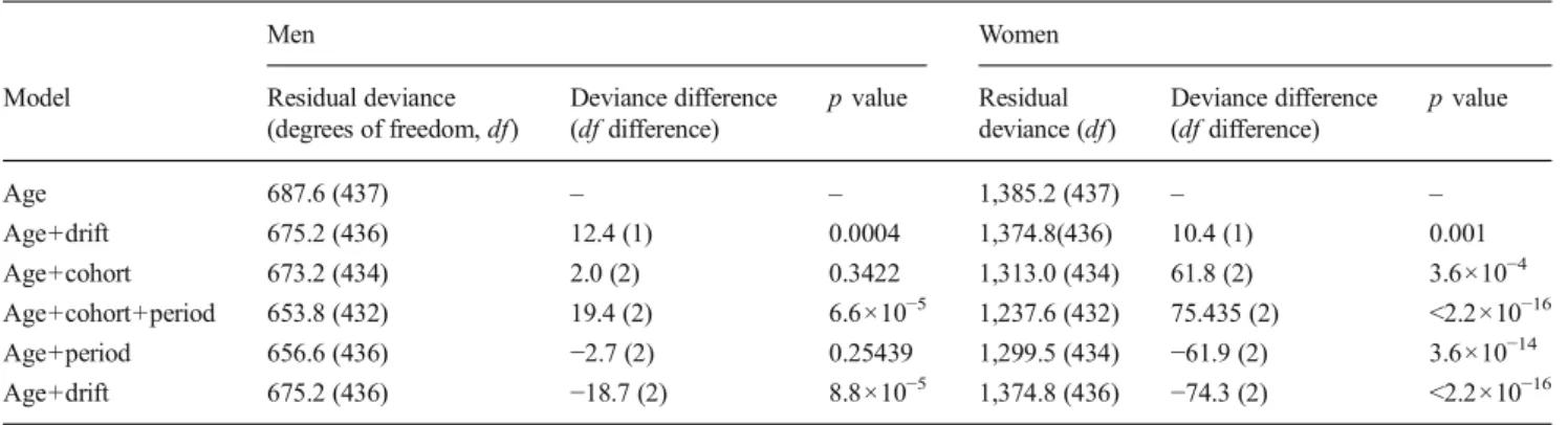
The results from the use of apc.fit are shown in Tables2and3

and Fig. 1; Table 2shows all possible models with the APC

effects. By comparing the deviance between adjacent lines (a lower p value indicates a better fit), it was possible to identify which model provided a better fit. For women, the best fit is achieved by use of the full APC model whereas in men, the best

fit is obtained by use of the age–period model. Table3shows the

estimated rate ratios relative to cohort 1920 for both men and women, using the APC model, for apc.fit. For the parameteriza-tion used, the rate ratios (RR) in women varied between an estimated decrease risk of 57 % in the 1958 birth cohort to an increased risk of 19 % in the 1934, 1935 and 1936 birth cohorts. In men, the estimated RR varied between a decreased risk of 5 % in 1904–1910 (although not statistically significant) to an

in-creased risk of 42 % in the 1956 birth cohorts. Figure1is divided

into three plots, where the effects are displayed for both genders (women in black and men in light grey). The left plot presents the age effect with the display of age-specific incidence rates for 100,000 person–years. The centre plot is the graphic display of

the cohort effect (numerically displayed in Table3). Finally, the

right plot presents the period effect as residual ratio rates. The effect of all parameters—age, period and cohort on hip

Ta b le 1 Age-specific crude inciden ce rates p er 100,000 pers on-years and 95 % confidence intervals, by sex, for each o f th e study period years 2000 –2 008 Sex A ge group s Pe ri od ye ar s 2 000 2 001 2002 2003 2004 2005 2006 2007 2008 Men 5 0– 54 13 .6 (9 .8 –18.2) 1 6 .5 (12.4 –21 .6) 14.2 (10.3 –19 .0) 19.6 (15.1 –2 5 .2) 17.0 (12.7 –2 2 .2) 15.5 (1 1 .4 –2 0 .5) 13.4 (9.6 –1 8 .2) 16.0 (1 1 .8 –2 1 .2) 19.7 (15.1 –25.2) 55 –59 22 .2 (1 7 .2 –28.1 ) 2 2 .0 (17.0 –28 .0) 17.9 (13.4 –23 .5) 25.6 (20.1 –3 2 .1) 25.9 (20.3 –3 2 .5) 29.1 (23.1 –36.3) 34.5 (27.8 –42.3) 32.7 (26.1 –40.4) 24.4 (19.0 0– 30.8) 60 –64 29 .9 (2 3 .7 –37.3 ) 4 7 .6 (30.5 –45 .8) 34.4 (27.5 –42 .4) 33.4 (26.6 –4 1 .4) 39.3 (31.8 –4 8 .0) 36.3 (29.2 –44.8) 33.9 (27.0 –42.1) 39.0 (31.5 –47.7) 36.3 (29.5 –44.3) 65-69 7 2 .1 (61.5 –84.0 ) 8 4 .9 (73.4 –97 .8) 68.8 (58.5 –80 .4) 65.9 (55.9 –7 7 .2) 61.7(52.1 –72.6) 67.3 (57.3 –78.7) 65.0 (55.1 –76.2) 66.1 (56.1 –77.4) 54.2 (45.2 –64.5) 70 –7 4 1 04.0 (90.6 –1 1 8.8) 1 31.8 (1 16.6 –1 48.3) 108.2 (94.5 –1 23.4) 137.5 (121.9 –154.5) 1 13.3 (99.1 –1 29.0) 120.4 (105 .6 –136.7) 127.6 (1 12.2 –144.5) 1 10.4 (96.0 –126.4) 108.4 (94 .6 –123.8) 75 –7 9 2 26.1 (203.4 –2 50.5) 2 31.6 (208.4 –256.7) 220.8 (197.8 –245.7) 259.4 (234.1 –286.7) 240.5 (216.0 –267.1) 237.4 (212 .9 –264.1) 280.7 (253 .8 –309.8) 228.2 (20 3.7 –254.8 ) 251.3 (22 6.9 –277.6 ) 80 –8 4 3 46.2 (310.3 –3 85.1) 4 05.3 (365.9 –447.7) 410.9 (370.8 –454.1) 463.9 (420.8 –510.3) 492.8 (447.5 –541.4) 527.4 (479 .4 –578.9) 583.7 (531 .9 –639.2) 598.5 (54 4.6 –656.3 ) 492.6 (44 7.4 –541.2 ) 85 –8 9 8 91.3 (795.3 –9 95.8) 8 96.3 (801.6 –999.2) 794.9 (707.5 –890.2) 932.1 (839.2 –1,032.6) 889.4 (800.4 –985.7) 805.8 (722 .6 –896.1) 783.9 (703 .3 –871.4) 702.5 (62 7.8 –783.6 ) 870.8 (78 9.1 –958.7 ) 90 –9 4 1 ,398.0 (1,173.7 – 1 ,653.0) 1 ,486.0 (1,259 .1 – 1 ,742.2) 1,414.2 (1,197 .6 – 1,658.9) 1,166.3 (974 .5 – 1,385.2) 1,632.9 (1,40 9.0 – 1,882.6) 1,457.1 (1,25 0.4 – 1,688.5) 1,529.8 (1,322.1 –1,761.0) 1,397.1 (1,203.1 –1,613.8) 1,200 .6 (1 ,024.9 – 1,398 .0 ) 95 –9 8 2 ,072.3 (1 ,353.7 –3,0 36.3) 2 ,106.8 (1,41 1.1 – 3 ,025.7) 2,382.5 (1,668 .7 – 3,298.4) 1,506.2 (974 .7 – 2,223.4) 2,358.3 (1,70 6.7 – 3,176.7) 1,995.8 (1,425.9 –2,717.8) 2,269.1 (1,6 84.2 – 2,991.6 ) 1,610.0 (1,148.9 –2,200.9) 1,426 .1 (1,009.2 –1,957.4) Wo m en 5 0– 54 13 .6 (1 0 .0 –18.1 ) 1 3 .8 (10.1 –18 .3) 15.1 (1 1 .2 –19.8 ) 18.4 (14.1 –2 3 .6) 1 1.7 (8.3 –16.0 ) 16.3 (12.3 –21.3) 13.4 (9.8 –1 8 .0) 13.4 (9.7 –1 8 .0) 13.5 (9.5 –18.0) 55 –59 27 .1 (2 1 .7 –33.3 ) 2 8 .5 (23.0 –34 .9) 23.3 (18.3 –29 .2) 32.7 (26.7 –3 9 .6) 24.9 (19.7 –3 1 .1) 30.3 (24.5 –37.1) 27.4 (21.8 –34.0) 21.6 (16.6 –27.6) 25.9 (20.6 –32.1) 60 –64 50 .5 (4 2 .8 –59.1 ) 5 7 .2 (48.9 –66 .5) 51.6 (43.7 –60 .5) 57.7 (49.2 –6 7 .2) 54.8 (46.5 –6 4 .3) 51.4 (43.3 –60.6) 62.6 (53.6 –72.7) 55.9 (47.5 –65.4) 50.4 (42.7 –59.1) 65 –6 9 1 27.0 (1 13.9 –1 41.2) 1 27.6 (1 14.5 –1 41.8) 127.8 (1 14.8 –1 42.0) 135.4 (122.1 –149.8) 1 18.5 (106.1 –132.0) 1 12.5 (100.5 –125.6) 109.8 (97.9 –122.8) 98.7 (87.4 –1 1 1.1) 86.7 (76.1 –98.3) 70 –7 4 2 95.2 (274.9 –3 16.6) 3 1 1.2 (290.4 –3 33.2) 248.9 (230.2 –268.6) 280.7 (260.8 –301.8) 279.3 (259.3 –300.4) 257.7 (238 .4 –278.2) 279.2 (258 .9 –300.7) 250.2 (23 0.8 –270.7 ) 236.4 (21 8.1 –255.8 ) 75 –7 9 5 32.9 (503.3 –5 36.7) 5 74.1 (543.1 –606.4) 567.8 (536.6 –600.3) 622.6 (589.6 –656.9) 605.3 (572.5 –639.5) 615.5 (582 .2 –650.3) 634.8 (600 .6 –670.4) 604.1(5 70.3 –639 .4) 567.8 (53 6.7 –600.2 ) 80 –8 4 8 23.5 (780.1 –8 68.8) 9 14.2 (867.8 –962.5) 932.5 (884.9 –982.1) 1,085.6 (1,033 .4 – 1,139.8) 1,189.2 (1,13 3.5 – 1,246.9) 1,294.8 (1,23 5.2 – 1,356.4) 1,340.0 (1,2 77.9 – 1,404.4 ) 1,380.4 (1,315.7 –1,447.4) 1,133 .3 (1,079.6 –1,188.9) 85 –8 9 1 ,871.7 (1 ,771.4 –1,9 76.3) 1 ,983.6 (1 ,882.1 –2,0 89.2) 1,900.5 (1,802.9 –2 ,0 02.1) 1,853.7 (1,759 .1 – 1,952.1) 1,687.4 (1,59 9.0 – 1,779.5) 1,721.2 (1,633.6 –1,812. 7) 1,683.8 (1,5 98.3 – 1,772.8 ) 1,642.4 (1,559.6 –1,728.4) 1,747 .9 (1,664.1 –1,834.7) 90 –9 4 2 ,728.5 (2 ,525.2 –2,9 43.9) 2 ,740.5 (2 ,540.7 –2,9 52.0) 2,736.0 (2,540.2 –2 ,9 43.0) 2,804.0 (2,609 .6 – 3,009.2) 3,198.1 (2,99 4.2 – 3,412.3) 2,929.0 (2,737.8 –3,130.1) 2,724.4 (2,5 43.7 – 2,914.7 ) 2,506.4 (2,336.6 –2,685.4) 2,524 .7 (2,357.5 –2,700.7) 95 –9 8 2 ,750.5 (2 ,284.1 –3,2 84.8) 3 ,481.9 (2 ,972.4 –4,0 54.3) 3,063.3 (2,602.9 –3 ,5 82.3) 3,139.8 (2,689 .4 – 3,644.7) 3,325.6 (2,87 7.4 – 3,824.2) 2,700.0 (2,31 1 .6 –3 ,135.5) 3,166.8 (2,7 59.5 – 3,617.7 ) 2,618.3 (2,2 61.9 – 3,015.2 ) 3,076 .6 (2,702.7 –3,488.2)

GAM analysis. Age effects are similar for both genders, whereas the period effect is different: a falling pattern in women after 2004 and a fluctuating pattern in men. The cohort effect between 1920 and 1940 presents a similar statistically significant pattern in both sexes: increasing risk until 1930 followed by a decreasing risk to about 1940. Even though the patterns are not statistically significant after 1940, both sexes present an increase, which in women is interrupted by another fall around 1950. The models explained 98 and 99.1 % of the deviance for men and women respectively and, for both, all smooth terms (A , P and C ) were statistically significant.

Discussion

A cohort effect on hip fracture incidence rates in Portugal was observed with risk fluctuations in men and women born at times of major political and economic changes as can be seen

in Fig.3, where the historical curve of consumer price index

and chronogram of political and economic changes in Portugal are displayed, together with the curves of cohort effect in men and women. Poor nutritional and health condi-tions in intrauterine life and childhood could be a plausible explanation for the increased risk in cohorts born in times of Table 2 Results from age-period-cohort effects modelling

Men Women

Model Residual deviance

(degrees of freedom, df) Deviance difference (df difference) p value Residual deviance (df) Deviance difference (df difference) p value Age 687.6 (437) – – 1,385.2 (437) – – Age+drift 675.2 (436) 12.4 (1) 0.0004 1,374.8(436) 10.4 (1) 0.001 Age+cohort 673.2 (434) 2.0 (2) 0.3422 1,313.0 (434) 61.8 (2) 3.6×10−4 Age+cohort+period 653.8 (432) 19.4 (2) 6.6×10−5 1,237.6 (432) 75.435 (2) <2.2×10−16 Age+period 656.6 (436) −2.7 (2) 0.25439 1,299.5 (434) −61.9 (2) 3.6×10−14 Age+drift 675.2 (436) −18.7 (2) 8.8×10−5 1,374.8 (436) −74.3 (2) <2.2×10−16

Table 3 Rate ratios (RR) of birth cohorts and 95 % CI relative to 1920 for men and women

Cohort Men Women Cohort Men Women Cohort Men Women

RR (95 % CI) RR (95 % CI) RR (95 % CI)

1902 0.96 (0.77–1.19) 1.02 (0.91–1.13) 1921 1.01 (1–1.02) 1.01 (1.01–1.01) 1940 1.33 (1.14–1.54) 1.12 (1.02–1.22) 1903 0.96 (0.78–1.17) 1.01 (0.92–1.11) 1922 1.02 (1.01–1.03) 1.02 (1.01–1.03) 1941 1.34 (1.15–1.56) 1.09 (0.99–1.19) 1904 0.95 (0.79–1.15) 1 (0.92–1.1) 1923 1.03 (1.01–1.05) 1.04 (1.02–1.05) 1942 1.35 (1.15–1.59) 1.05 (0.95–1.16) 1905 0.95 (0.8–1.13) 1 (0.92–1.09) 1924 1.05 (1.02–1.08) 1.05 (1.04–1.07) 1943 1.36 (1.15–1.61) 1.02 (0.91–1.13) 1906 0.95 (0.81–1.12) 0.99 (0.92–1.07) 1925 1.06 (1.03–1.1) 1.07 (1.05–1.09) 1944 1.37 (1.15–1.63) 0.98 (0.87–1.09) 1907 0.95 (0.83–1.1) 0.99 (0.92–1.06) 1926 1.08 (1.03–1.12) 1.08 (1.06–1.11) 1945 1.38 (1.15–1.65) 0.93 (0.83–1.06) 1908 0.95 (0.84–1.09) 0.98 (0.93–1.05) 1927 1.09 (1.04–1.15) 1.1 (1.07–1.13) 1946 1.38 (1.14–1.68) 0.89 (0.78–1.02) 1909 0.95 (0.85–1.07) 0.98 (0.93–1.04) 1928 1.11 (1.05–1.18) 1.12 (1.08–1.16) 1947 1.39 (1.14–1.7) 0.85 (0.73–0.98) 1910 0.95 (0.86–1.06) 0.98 (0.93–1.03) 1929 1.13 (1.06–1.21) 1.14 (1.1–1.18) 1948 1.4 (1.13–1.73) 0.8 (0.69–0.94) 1911 0.96 (0.87–1.04) 0.97 (0.93–1.02) 1930 1.15 (1.07–1.24) 1.15 (1.1–1.2) 1949 1.4 (1.12–1.75) 0.76 (0.64–0.9) 1912 0.96 (0.89–1.03) 0.97 (0.94–1.01) 1931 1.17 (1.08–1.27) 1.17 (1.11–1.22) 1950 1.4 (1.11–1.78) 0.72 (0.6–0.86) 1913 0.96 (0.9–1.02) 0.97 (0.94–1) 1932 1.19 (1.08–1.3) 1.18 (1.12–1.24) 1951 1.41 (1.09–1.81) 0.67 (0.55–0.82) 1914 0.96 (0.91–1.02) 0.97 (0.95–1) 1933 1.21 (1.09–1.33) 1.19 (1.12–1.25) 1952 1.41 (1.08–1.84) 0.63 (0.51–0.79) 1915 0.97 (0.93–1.01) 0.97 (0.95–0.99) 1934 1.23 (1.1–1.37) 1.19 (1.12–1.26) 1953 1.41 (1.06–1.87) 0.59 (0.47–0.75) 1916 0.97 (0.94–1) 0.98 (0.96–0.99) 1935 1.25 (1.11–1.4) 1.19 (1.12–1.27) 1954 1.41 (1.05–1.91) 0.56 (0.44–0.71) 1917 0.98 (0.95–1) 0.98 (0.97–0.99) 1936 1.26 (1.12–1.43) 1.19 (1.11–1.27) 1955 1.42 (1.03–1.94) 0.52 (0.4–0.68) 1918 0.98 (0.97–1) 0.99 (0.98–0.99) 1937 1.28 (1.13–1.46) 1.18 (1.1–1.27) 1956 1.42 (1.01–1.98) 0.49 (0.37–0.65) 1919 0.99 (0.98–1) 0.99 (0.99–1) 1938 1.3 (1.13–1.49) 1.16 (1.08–1.26) 1957 1.42 (0.99–2.02) 0.46 (0.34–0.61) 1920 Reference Reference 1939 1.31 (1.14–1.51) 1.14 (1.05–1.24) 1958 1.42 (0.98–2.06) 0.43 (0.31–0.58)

deprivation and similarly investments in health and wellbeing could explain the fall in risk in cohorts born in times of political stability. In women, the cohort effect was marked by a tendency of an increase in risk until 1930 followed by a

decrease in risk (Figs.1and2). Even though not statistically

significant, there were inflections in risk in 1920 (from stable to increasing), 1940 (from decreasing to increasing) and in

1950 (from increasing to decreasing; Fig.2). Similar results

were observed for men except for 1950, when the decreasing risk trend was not observed. Women in younger cohorts presented lower risk, while for men the estimated risk in

younger cohorts was higher (Table2).

Regardless of an existing cohort effect, there was a period effect in women with a marked turning point in 2004, where the incidence rate decreased. This decrease could be the result of one or several factors mentioned in other studies (medication, prevention, changes in risk factors or changes in the

codifica-tion system) [16]. However, the most plausible reason for the

different period effect for men and women has been discussed

in a previous study with the same population [15] where we

identified a relationship between the number of anti-osteoporotic medication sales with the pattern of age-standardised incidence rates in women—the target population of the prescriptions. The current results confirm the existence of period effects even after adjusting for age and cohort effects. The age effect was similar in both sexes, with an exponential-like age increase, as expected and reported in most of the studies.

Current literature is scarce on studies that analyse the effects of time on the three different scales (age, period and cohort) and comparisons must be carefully interpreted because of differences

in methodologies. Nevertheless, New Zealand [7] and Sweden

[8] have reported a continuous decrease in risk for younger

cohorts but contrasting period effects with New Zealand show-ing a continuous increase versus a continuous decrease in

Sweden. A recent study in Canada [10] also identified a

decreased risk in younger cohorts and a non-linear effect of cohort in men. However, unlike our study, no fluctuations in risk were identified for birth cohorts. All studies have pointed to possible changes in risk factors as drivers of the observed trends. Nevertheless, they also point to some aspects that follow our reasoning. The New Zealand study points out that the cohort effect can be different in countries with a different social history, while the Swedish study briefly describes the history of the country as a means of understanding the results observed. The age effects were consistent with established knowledge: risk increased exponentially with age. Two other studies attempt to report the time effects separately: one uses a methodology that

cannot produce comparable results with ours [29] while another

uses data from older periods 1968–1986 [9].

Hip fractures can be a consequence of balance between

formation and resorption in bone tissue throughout life [4].

Therefore, we can argue that hip fractures are a consequence of lifetime exposure rather than the result of short-period exposure. The quality of life in youth can be a particular determinant in the quality of bones, and osteoporosis was until a few years ago considered a paediatric disease with clinical

manifestation in the elderly [30]. Heaney et al. [30] described

the bone mass lifeline where the maximum bone mass poten-tial achieved by hereditary factors can be altered by several environmental factors. In addition, intrauterine development

is a determinant in adult bone mass pick [5,6]. Bone growth in

the uterus demands suitable nutrients supplied via maternal food intake. Periods of political and economic changes influ-ence population health; the twentieth century was replete with major conflicts, particularly in Portugal.

The first three decades of the twentieth century in Portugal were marked by internal and external causes of instability with an impact on the population’s quality of life. Portugal was still recovering from the political change from a Monarchy to a Republic (1908–1910) when, in 1914, the First World War Fig. 1 Estimated effects (and 95 % CI) for hip fracture incidence rate using the apc.fit (women black, men light grey). Age effect in the left plot, cohort effect in the centre plot and period effect in the right plot

(WWI, 1914–1918) was declared with Portugal playing an active part with the Allies. During the war, in 1917 and 1918, there was a food shortage in Portugal and after that the popula-tion had to face the Spanish flu (1918 and 1919). The post-WWI period in Portugal was marked by increasing inflation, among the highest in Europe, aggravated by political instability. Portugal was amongst the poorest and unhealthiest countries in

Europe [31]. See Fig. 2 (cohort effect) for compatible risk

alterations in the incidence of hip fractures during this period. From 1927 to 1933, a new major political change marked the history of the nation. The Republic was replaced by a provisional authority, led by the military, followed by a totali-tarian regime that lasted 41 years. In the 1930s, political stabil-ity was achieved, finances and economy were reorganised and

investments were made for the construction of thousands of elementary schools, hospitals, health centres and infrastructures such as roads, electricity and sewage. Portugal saw a

progres-sive improvement in the general quality of life. Figure2(cohort

effect) shows compatible risk alterations around this period. The decreasing risk of hip fractures observed in cohorts born in the 1930s turned to another period of risk increasing after 1940. In spite of the neutral part that Portugal played in the Second World War (WWII, 1939–1945), there were eco-nomic, social and political effects, mainly because Portugal

depended on warring countries’ imports of fuel, industrial

primary resources and food. After WWII, there was a boost in the European economy with the Marshall Plan (1948– 1951). Portugal received the funds in 1949, which were

mostly used for the purchase of food supplies. In 1952, Portugal implemented the 1st Foment Plan to improve living

conditions and productivity, reduce unemployment [31] and

speed up the industrialization of the country. At that time, Portugal was mainly a rural society and industrialization started a process of rural exodus. Nevertheless, Portugal was still among the poorest countries in Europe and the isolation of the totalitarian government prevented the country from fol-lowing the post-WWII development of other west European countries. The solution to escaping poverty, for many Portuguese, was to emigrate. The 1950s was a period of intense emigration, mainly of young men, especially to France and Germany. Their cash remittances helped not only to improve the wellbeing of their families in Portugal but also the industrialization of the country. Meanwhile the emigrants themselves were living in very poor conditions. This could be a possible explanation for the gender risk inequalities for cohorts born after 1950 observed in our results: for men, the risk continued to increase while for women, it started to decrease. However, data for a longer period need to be analysed in future studies in order to improve the estimates for younger cohorts.

Causal effect in epidemiology has been thoroughly

discussed and analysed [32]. Observational studies lack the

criteria of causality and therefore results are commonly overlooked. It is difficult to attribute causal effects on hip

fracture incidence due to the intrinsic nature of bone health, reflecting a lifetime of exposure. However, our results pinpointed a number of aspects that can be seen as indicators of causality. In addition, there was a reasonable match be-tween the cohort effect and historical data of the consumer

price index (Fig. 3, where the historical events were also

overlaid), which reflects the standard of living and measures the changing costs of purchasing goods and services, often

used as an indicator of living standards [33]. It is accepted that

conditions during the period where bone formation surpasses bone resorption, including intrauterine growth, have impacts

on bone health later in life [5,30]. Hence, the similar cohort

effect observed in both genders, with changes in each and every single period of time where a major historical event

occurs (Fig. 2 cohort effect and Fig. 3), should not be

overlooked on the basis of lack of strong association or of disregarding other causal factors. Nevertheless, we are not postulating causality nor that the cohort effect is a necessary

or a sufficient cause [32] in understanding trends in hip

fracture incidence, but it seems an important factor to be analysed in future studies. The fact that risk alterations and historical events are simultaneous backs up the hypothesis of the importance of nutrient availability during uterine growth as much as conditions during childhood and adolescence.

The mechanism that drives the secular trends of hip fractures

is complex [34] and therefore its understanding benefits from the

use of different and new approaches. The inherent limitations of studies using the APC models that are related to the identifiability problem and that invalidate any quantification of the different effects do not override the importance of the results obtained. We have chosen to fit a full APC GAM model for men as well, even though the apc.fit analysis showed that a more accurate fit would be the age–period model, because this was acknowledging an important aspect of the cohort effect that would otherwise have been disregarded. In addition, it allowed a gender comparison. The strength of our study relies on addressing age, period and cohort effects simultaneously from several methodology per-spectives and using nationwide population-based data.

In this study, an innovative perspective on the reasons that drive the trends of hip fracture incidence rates is presented, highlighting the considerable differences in the populations at risk of sustaining a hip fracture. There was a fluctuation in hip risk in both men and women born at times of major political and economic changes, regardless of period effects, which could be related to the nutritional and health conditions in Portugal at the time.

Acknowledgments This work was supported by FEDER funds through

the Programa Operacional Factores de Competitividade (COMPETE) and by Portuguese funds through Fundação para a Ciência e a Tecnologia (FCT) within the framework of the project PEst-C/SAU/LA0002/2011 and by PTDC/SAU-EPI/113424/2009 grant and SFRH/BD/40978/2007 fellowship. We like to acknowledge the Central Administration of Health Services (ACSS) for the data from the National Hospital Discharge Register. We also like to acknowledge Paulo Nossa for helping with the understanding of economic, social and political history of Portugal.

Conflict of Interests None.

References

1. Hopkins RB, Goeree R, Pullenayegum E, Adachi JD, Papaioannou A, Xie F, Thabane L (2011) The relative efficacy of nine osteoporosis medications for reducing the rate of fractures in post-menopausal

women. BMC Musculoskelet Disord 12:209. doi:

10.1186/1471-2474-12-209

2. Ioannidis G, Flahive J, Pickard L, Papaioannou A, Chapurlat RD, Saag KG, Silverman S, Anderson FA Jr, Gehlbach SH, Hooven FH, Boonen S, Compston JE, Cooper C, Diez-Perez A, Greenspan SL, Lacroix AZ, Lindsay R, Netelenbos JC, Pfeilschifter J, Rossini M, Roux C, Sambrook PN, Siris ES, Watts NB, Adachi JD (2012) Non-hip, non-spine fractures drive healthcare utilization following a frac-ture: the Global Longitudinal Study of Osteoporosis in Women

(GLOW). Osteoporos Int. doi:10.1007/s00198-012-1968-z

3. Kanis JA (2002) Diagnosis of osteoporosis and assessment of

frac-ture risk. Lancet 359(9321):1929–1936. doi:

10.1016/s0140-6736(02)08761-5

4. Hunter DJ, Sambrook PN (2000) Bone loss: epidemiology of bone

loss. Arthritis Res 2(6):441–445. doi:10.1186/ar125

5. Cooper C, Westlake S, Harvey N, Javaid K, Dennison E, Hanson M (2006) Review: developmental origins of osteoporotic fracture.

Osteoporos Int 17(3):337–347. doi:10.1007/s00198-005-2039-5

6. Baird J, Kurshid MA, Kim M, Harvey N, Dennison E, Cooper C (2011) Does birthweight predict bone mass in adulthood? A

systematic review and meta-analysis. Osteoporos Int 22(5):1323–

1334. doi:10.1007/s00198-010-1344-9

7. Langley J, Samaranayaka A, Davie G, Campbell AJ (2011) Age, cohort and period effects on hip fracture incidence: analysis and

predictions from New Zealand data 1974–2007. Osteoporos Int

22(1):105–111. doi:10.1007/s00198-010-1205-6

8. Rosengren B, Ahlborg H, Mellstrom D, Nilsson J, Bjork J, Karlsson

M (2012) Secular trends in Swedish hip fractures 1987–2002: birth

cohort and period effects. Epidemiology 23(4):623–630

9. Evans JG, Seagroatt V, Goldacre MJ (1997) Secular trends in prox-imal femoral fracture, Oxford record linkage study area and England

1968–86. J Epidemiol Commun Health 51(4):424–429

10. Jean S, O’Donnell S, Lagace C, Walsh P, Bancej C, Brown JP, Morin

S, Papaioannou A, Jaglal SB, Leslie WD (2013) Trends in hip

fracture rates in Canada: an age–period–cohort analysis. J Bone

Miner Res 28(6):1283–1289. doi:10.1002/jbmr.1863

11. Cumming RG, Nevitt MC, Cummings SR (1997) Epidemiology of

hip fractures. Epidemiol Rev 19(2):244–257

12. Fisher A, Martin J, Srikusalanukul W, Davis M (2010) Bisphosphonate use and hip fracture epidemiology: ecologic proof from the contrary.

Clin Interv Aging 5:355–362. doi:10.2147/cia.s13909

13. Reginster JY, Kaufman JM, Goemaere S, Devogelaer JP, Benhamou CL, Felsenberg D, Diaz-Curiel M, Brandi ML, Badurski J, Wark J, Balogh A, Bruyere O, Roux C (2012) Maintenance of antifracture efficacy over 10 years with strontium ranelate in postmenopausal osteoporosis.

Osteoporos Int 23(3):1115–1122. doi:10.1007/s00198-011-1847-z

14. Fisher AA, O’Brien ED, Davis MW (2009) Trends in hip fracture epidemiology in Australia: possible impact of bisphosphonates and

hormone replacement therapy. Bone 45(2):246–253. doi:10.1016/j.

bone.2009.04.244

15. Alves SM, Economou T, Oliveira C, Ribeiro AI, Neves N, Goméz-Barrena E, Pina MF (2013) Osteoporotic hip fractures: bisphosphonates sales and observed turning point in trend. A population-based retrospec-tive study. Bone 53(2):430–436

16. Cooper C, Cole ZA, Holroyd CR, Earl SC, Harvey NC, Dennison EM, Melton LJ, Cummings SR, Kanis JA (2011) Secular trends in the incidence of hip and other osteoporotic fractures. Osteoporos Int

22(5):1277–1288. doi:10.1007/s00198-011-1601-6

17. Barros P, de Almeida Simões J (2007) Portugal: Health system review, vol 9 (5). Health Systems in Transition. WHO Regional Office for Europe

18. ACSS (2011) Auditoria da codificação clínica [Clinical codification

Audits].http://portalcodgdh.min-saude.pt/index.php/Auditoria_da_

codificação_cl%C3%ADnica. 2012

19. Melton LJ 3rd, Kearns AE, Atkinson EJ, Bolander ME, Achenbach SJ, Huddleston JM, Therneau TM, Leibson CL (2009) Secular trends

in hip fracture incidence and recurrence. Osteoporos Int 20(5):687–

694. doi:10.1007/s00198-008-0742-8

20. INE (2012) Instituto Nacional de Estatística. 2011

21. Carstensen B (2007) Age–period–cohort models for the Lexis

dia-gram. Stat Med 26(15):3018–3045. doi:10.1002/sim.2764

22. Morris JA, Gardner MJ (2000) Epidemiological studies. In: Altman DG, Machin D, Bryant TN, Gardner MJ (eds) Statistics with confi-dence, second edition ed. BMJ Books, Bristol

23. Faraway JJ (2006) Extending the linear model with R: generalized linear, mixed effects and nonparametric regression models. Texts in statistical science series. Chapman & Hall, Boca Raton

24. Carstensen B, Plummer M, Laara E, Hills M (2012) Epi: a package for Statistical analysis in epidemiology. R package version 1.1.40 ed 25. Holford TR (1983) The estimation of age, period and cohort effects

for vital rates. Biometrics 39:311–324

26. Clements MS, Armstrong BK, Moolgavkar SH (2005) Lung cancer rate predictions using generalized additive models. Biostatistics

6(4):576–589. doi:10.1093/biostatistics/kxi028

27. Hastie T, Tibshirani R (1995) Generalized additive models for

28. Wood SN (2011) Fast stable restricted maximum likelihood and marginal likelihood estimation of semiparametric generalized linear

models. J R Stat Soc (B) 73(1):3–36

29. Samelson EJ, Zhang Y, Kiel DP, Hannan MT, Felson DT (2002) Effect of birth cohort on risk of hip fracture: age-specific incidence

rates in the Framingham Study. Am J Public Health 92(5):858–862

30. Heaney RP, Abrams S, Dawson-Hughes B, Looker A, Marcus R, Matkovic V, Weaver C (2000) Peak bone mass. Osteoporos Int

11(12):985–1009

31. História de Portugal [History of Portugal] (1994). Círculo de Leitores 32. Rothman KJ, Greenland S (2005) Causation and causal inference in

epidemiology. Am J Public Health 95(Suppl 1):S144–S150. doi:10.

2105/ajph.2004.059204

33. INE (2001) Estatísticas Históricas Portuguesas [Historical statistics in Portugal].

34. Melton LJ 3rd, O’Fallon WM, Riggs BL (1987) Secular

trends in the incidence of hip fractures. Calcif Tissue Int