Effects of landslide inventories uncertainty on landslide susceptibility modelling
6
0
0
Texto
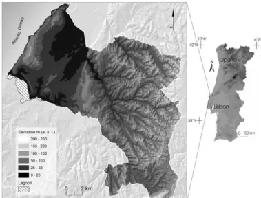
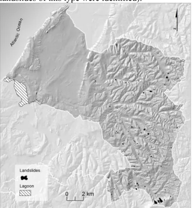
(2) 2 STUDY AREA The study was performed in the Caldas da Rainha County. The test site has 256 km2 and its elevation ranges from 0 to 260 m (Fig. 1). The Óbidos Lagoon is located in the SW part of the County, and it is a geomorphologic heritage attesting the Holocene shore zone of Central Portugal. The regional geology includes rocks dated from the Triassic to the Quaternary (Fig. 2). Triassic rocks are the “Dagorda” marls and clays, which are constrained to a NE-SW direction diapyric anticline located in the west part of the study area. During Quaternary, the diapyric zone evolved to a graben, and the Dagorda marls and clays have been subjected to erosion (Zêzere 2005). Therefore, a smooth, low altitude (<50 m) basin was created (Fig. 1).. dolerite outcrops in the south zone of the county (Fig. 2). From the geomorphologic point of view, the area located eastwards of the diapyr is a polygenic coastal plateau that was constructed during the Late Pliocene and the Early Quaternary (Ferreira 1981). The quaternary fluvial erosion was responsible for the degradation of the plateau and promoted the creation of some steep slopes (Zêzere 2005). The incised fluvial valleys have a typical SE-NW direction (e.g., the Tornada River), orthogonal to main regional geological structures (Figs. 1-2). The valley slopes are affected by rainfall-triggered landslides, mostly of the rotational slide type. Westward of the diapyr, rocks dated from the middle and the upper Jurassic are mostly limestones and marls, with sandstone intercalations (Fig. 2). From the geomorphologic point of view, this area is interpreted as a tectonic block belonging to the above mentioned coastal plateau, which was uplifted along the west-side diapyr fault (Zêzere 2005). Coastal cliffs up to 120m-high are present in this area, and they cut rocks dipping NW. Due to the favourable geometry, these cliffs evolve frequently by deep-seated translational slides developed alongside less-resistant boundary layers. 3 DATA AND METHODS 3.1 Landslide Inventory. Figure 1. Study area location and elevation.. Figure 2. Simplified lithological map of the study area.. Eastward of the diapyr, a NE-SW large syncline is present, and the upper Jurassic sandstones and claystones are dominant. Additionally, a 151 ha. Detailed geo-referenced digital ortophotomaps (pixel = 0.5 m) obtained in 2004 were combined with the accurate topography to build three different landslide inventories, even though landslide recognition was made without stereoscopic image interpretation. Landslides affecting coastal cliffs have particular geomorphological constrains and were not included in these landslide inventories, in order to avoid interference in the landslide susceptibility results. The landslide inventory #1 was constructed by a single regular-trained geomorphologist using photointerpretation. A total of 408 probable slope movements were identified and geo-referenced by a point marked in the central part of the probable landslide rupture zone (Fig. 3). The landslide inventory #2 was obtained through the examination of landslide inventory #1 by a senior geomorphologist. This second phase of photographic and morphologic interpretation (prevalidation) allowed the selection of 204 probable slope movements from the first landslide inventory (Fig. 4). The landslide inventory #3 was obtained by the field verification of the total set of probable landslide zones (408 points), and was performed by 6 geomorphologists. This inventory has 193 validated slope movements (Fig. 5), and includes 101 “new landslides” that have not been recognized - 82 -.
(3) by the ortophotomaps interpretation. Additionally, the field work enabled the cartographic delimitation of the slope movement depletion and accumulation zones, and the definition of landslide type.. inexistent in the inner part of the county (only two landslides of this type were identified).. Figure 5. Landslide inventory #3.. Figure 3. Landslide inventory #1.. Figure 4. Landslide inventory #2.. The total unstable area is 950,600 m2 and the landslide mean area is 4,875 m2. Rotational slides, both shallow and deep-seated, are the dominant landslide type (83% of total slope movements). Shallow translational slides represent 16% of total landslides, and the deep-seated translational slides, that are very frequent on coastal cliffs, are virtually. 3.2 Landslide Susceptibility Assessment Landslide susceptibility was assessed using independently the three landslide inventories. A single predictive model (logistic regression) was adopted and the same set of landslide predisposing factors was used to allow comparison of results. The logistic regression is a multivariate statistical method particularly robust to assess the spatial relationship between a dichotomous dependent variable (landslides) and a set of independent explanatory variables (landslide predisposing factors). This technique has been widely used worldwide with good results for landslide susceptibility evaluation (e.g., Dai & Lee 2003, Süzen & Doyuran 2004, Gorsevski et al. 2006, Carrara et al. 2008). Landslide predisposing factors are the following: slope angle (9 classes), slope aspect (9 classes), lithology (9 classes) and land use (6 classes). Probable landslides within landslide inventories #1 and #2 were marked as points. Therefore, in order to allow comparison, we extract the coordinates of the centroid of each landside depletion zone in landslide inventory #3, which were converted into a point for modelling purposes. Uncertainty associated to landslide inventory errors and their propagation on landslide susceptibility results are evaluated and compared by the construction of success-rate and prediction-rate curves and trough the computation of the respective AUC (Area Under Curve). The error derived from landslide inventories is quantified by assessing the overlapping degree of susceptible areas obtained from the different prediction models. - 83 -.
(4) 4 RESULTS AND DISCUSSION The landslide inventory #3 is the most reliable and accurate, as it is based on systematic landslide verification in the field. Therefore, this landslide inventory can be compared with the others to evaluate their errors. Landslide inventory #1 includes 408 probable landslide locations, but only 92 cases were confirmed to be slope movements by field work. Therefore, the true positive rate of this landslide inventory is only 22.5%. On the other hand, the landslide inventory #2 has less probable landslide locations (204), and as a consequence, the observed true positive rate is higher (45.1%) when compared with landslide inventory #1. Another source of uncertainty within landslide inventories #1 and #2 is the existence of landslides in the study area that have not been identified by photo interpretation. This source of error may be very relevant as these landslides correspond to 52.3% of total slope movements within landslide inventory #3. The large mismatch between the image interpretation (landslide inventories #1 and #2) and field mapping (landslide inventory #3) may be explained by the lack of stereoscopic photo interpretation. Figures 6-8 show the landslide susceptibility maps obtained using the logistic regression method, and by integrating, respectively, landslide inventories #1, #2 and #3 with the total set of landslide predisposing factors. For each simulation we use one cell per depletion zone and by landslide.. constrain, we do not compare the absolute logistic regression scores obtained from the three prediction models. Our attention was focused on the distribution of the most landslide susceptible areas predicted by each model.. Figure 7. Landslide susceptibility map [2] obtained with landslide inventory #2.. Figure 8. Landslide susceptibility map [3] obtained with landslide inventory #3.. Figure 6. Landslide susceptibility map [1] obtained with landslide inventory #1.. It is known that logistic regression results are sensitive to the number of cells (landslides) included in the model. Therefore, in order to avoid this. In order to allow a visual comparison, the three landslide susceptibility maps were classified using the same strategy: 4 susceptibility classes representing a fixed fraction of the total study area, which were defined after sorting, in a descending. - 84 -.
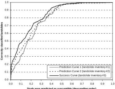
(5) way, the susceptibility scores computed for each pixel. When comparing figures 6-8, we conclude that there exists a very high level of similarity regarding landslide susceptibility results, despite differences existing among landslide inventories used to model susceptibility. The three landslide models classify as more susceptible those valley slopes located in the east part of the test site. Additionally, the most susceptible values are systematically assigned to slopes covering dolerite rocks next to the south limit of the study area. In order to quantify the propagation of landslide inventories errors on landslide susceptibility results, we compute the corresponding prediction-rate and success-rate curves (Chung & Fabbri 2003). This was made using a cross validation technique, by overlapping the landslide areas within landslide inventory #3 on the landslide susceptibility maps [1, 2, 3]. Therefore, we obtain a success-curve for the landslide susceptibility model produced with landslide inventory #3, because the same landslide data set is used to build the model and to validate it. Curves validating landslide susceptibility models build with landslide inventories # 1 and #2 can be interpreted as prediction-curves, because the landslide validation group (slope movements within landslide inventory #3) is independent relative to landslide modelling groups. 1.0. AUC is minimum for Map [1] (0.794) and maximum for Map [3] (0.840). Table 1. Area Under Curve (AUC) and prediction and success rate values for landslide susceptibility models. _________________________________________________ Area classified as susceptible (% of total area) __________________________________ 5 10 20 30 40 100 AUC ___________________________________________ Map [1] 0.20 0.31 0.53 0.75 0.85 1.0 0.794 Map [2] 0.29 0.39 0.61 0.76 0.88 1.0 0.810 Map [3] 0.34 0.48 0.66 0.78 0.93 1.0 0.840 __________________________________________________. Finally, we assess the uncertainty derived from landslide inventories errors by verifying the overlap degree of susceptible areas predicted by the three models. Table 2 summarizes the obtained results, and shows that overlapping degree among the three models is 52.2% for the 10% of total area classified as more prone to landslide occurrence. The overlap increase to 62.9% and 60.8%, when we consider, respectively, the 20% and 30% of total area classified as more prone to landslide occurrence. Table 2. Levels of conformity resulting from the overlap of landslide susceptibility maps [1, 2, 3]. ______________________________________________ Area classified as landslide Total overlapping susceptible expressed as % among maps [1, 2, 3] of total area ______________________________________________ 10 52.2 % 20 62.9 % 30 60.8 % ______________________________________________. 0.9. 5 CONCLUSION. Correctly classified landslides. 0.8 0.7 0.6 0.5 0.4 0.3 0.2 Prediction Curve 1 (landslide inventory #1) Prediction Curve 2 (landslide inventory #2). 0.1. Success Curve (landslide inventory #3) 0.0 0.0. 0.1. 0.2. 0.3. 0.4. 0.5. 0.6. 0.7. 0.8. 0.9. 1.0. Study area predicted as susceptible (descending order). Figure 9. Prediction-rate curves and success-rate curve corresponding to landslide susceptibility models obtained using landslide inventories # 1, #2 and #3.. Figure 9 shows the above mentioned predictionrate and success-rate curves. These curves attest that, despite similarities between landslide susceptibility maps, there is an increment in the model prediction performance from map [1] to map [2] and from map [2] to map [3]. This increment can be quantified trough the computation of the corresponding Area Under Curve (Table 1): The. Uncertainty in landslide inventories may be very high, namely when the inventory is totally based on photo-interpretation. This is the case of landslide inventories #1 and #2, elaborated without field work, by a single regular-trained geomorphologist and by a senior geomorphologist, respectively. The true positive rate of these inventories, evaluated by comparison with landslide inventory #3 that was validated in the field, is of 22.5% and 45.1%, respectively. Additionally, 52% of the total slope movements inventoried in the field were not identified during the photo-interpretation phase, and this is another important source of uncertainty. The lack of stereoscopic image interpretation justifies, at least partially, the disparity between the photo interpretation and the field mapping. Anyway, the field work and the inquiry to the local population were absolutely decisive to landslide inventory in the study area, because of the frequent destruction of landslide evidences by human action. Although the observed differences within landslide inventories, they produced very similar landslide susceptibility maps (differences on AUC = - 85 -.
(6) 0.05). Therefore, we can conclude that probable landslides identified in inventories #1 and #2 that were not confirmed in the field (false positives) are located on slopes that show similar characteristics to those affected by landslide activity, in what concerns the landslide predisposing factors (e.g., slope angle and aspect, lithology and land use), and this is the reason why there is no unconformity between the predicted results and the distribution of “true” slope movements. Even though the above mentioned similarity, the susceptibility model based on the most consistent and precise landslide inventory (#3) evidence the higher predictive quality, pointing out the relevance of the field verification on landslide inventorying. Moreover, taking into account the large number of false positives within landslide inventories #1 and #2, the field work was absolutely decisive for the consistent validation of the landslides susceptibility models.. Guzzetti, F., Cardinali, M., Reichenbach, P. & Carrara, A. 2000. Comparing landslide maps: A case study in the upper Tiber River Basin, central Italy, Environmental Management 25(3): 247-363. Guzzetti, F., Carrara, A., Cardinali, M., & Reichenbach, P. 1999. Landslide hazard evaluation: a review of current techniques and their application in a multi-scale study, Central Italy, Geomorphology 31: 181-216. Soeters, R. & van Westen, C.J. 1996. Slope instability recognition, analysis and zonation. In A.K. Turner & R.L. Schuster (eds), Landslide investigation and mitigation: 129-177. Washington D.C.: National Research Council, Transportation Research Board Special Report 247. Süzen, M.L. & Doyuran, V. 2004. A comparison of the GIS based landslide susceptibility assessment methods: multivariate versus bivariate, Environmental Geology 45(5): 665-679. Zêzere, J.L. 2005.A Geomorfologia da região das Caldas da Rainha. In Aires-Barros (Coord.), Caldas da Rainha: património das águas. A Legacy of Waters: 57-65. Lisboa: Assírio & Alvim.. ACKNOWLEDGEMENTS The research of J.-L. Zêzere, R.A.C. Garcia, S.C. Oliveira and A. Piedade was supported by the Portuguese Foundation for Science and Technology (FCT) through project Maprisk – Methodologies for assessing landslide hazard and risk applied to municipal planning (PTDC/GEO/68227/2006). R.A.C. Garcia and S.C. Oliveira were also supported by the Portuguese Foundation for Science and Technology of the Portuguese Ministry of Science, Technology and Higher Education.. REFERENCES Ardizzone, F., Cardinali, M., Carrara, A., Guzzetti, F. & Reichenbach, P. 2002. Uncertainty and errors in landslide mapping and landslide hazard assessment, Natural Hazards and Earth System Science 2(1-2): 3-14. Carrara, A., Cardinali, M. & Guzzetti, F. 1992. Uncertainty in assessing landslide hazard and risk, ITC Journal 2: 172183. Carrara, A., Crosta, G.B. & Frattini, P. 2008. Comparing models of debris-flow susceptibility in the alpine environment, Geomorphology 94: 353-378. Chung, C.-J. & Fabbri, A.G. 2003. Validation of Spatial Prediction Models for Landslide Hazard Mapping, Natural Hazards 30: 451-472. Dai, F.C. & Lee, C.F. 2003. A spatiotemporal probabilistic modelling of storm-induced shallow landsliding using aerial photographs and logistic regression, Earth Surafce Processes and Landforms 28: 527–545. Ferreira, D. B. 1981. Carte Geomorphologique du Portugal. Lisboa: Centro de Estudos Geográficos Memórias 6. Galli, M., Ardizzone, F., Cardinali, M., Guzzetti, F. & Reichenbach, P. 2008. Comparing landslide inventory maps, Geomorphology 94: 268-289. Gorsevski, P.V., Gessler, P.E., Foltz, R.B. & Elliot, W.J. 2006. Spatial prediction of landslide hazard using logistic regression and ROC analysis. Transactions in GIS 10(3): 395-415. - 86 -.
(7)
Imagem
![Figure 8. Landslide susceptibility map [3] obtained with landslide inventory #3.](https://thumb-eu.123doks.com/thumbv2/123dok_br/19201510.953968/4.892.55.419.690.1091/figure-landslide-susceptibility-map-obtained-landslide-inventory.webp)
Documentos relacionados