Differential proteomics: a study in Medicago truncatula somatic embryogenesis

UNIVERSIDADE DE LISBOA

FACULDADE DE CIÊNCIAS

DEPARTAMENTO DE BIOLOGIA VEGETAL

Differential proteomics: a study in

Medicago truncatula somatic

embryogenesis

Miguel André Lourenço da Luz Ventosa

Master in Biologia Celular e Biotecnologia

2010

UNIVERSIDADE DE LISBOA

FACULDADE DE CIÊNCIAS

DEPARTAMENTO DE BIOLOGIA VEGETAL

Differential proteomics: a study in

Medicago truncatula somatic

embryogenesis

Thesis oriented by Professor Pedro Fevereiro and André Almeida PhD

Miguel André Lourenço da Luz Ventosa

Biologia Celular e Biotecnologia

2010

Resumo

As leguminosas são um importante grupo de cultivares, utilizadas como alimento humano e animal, principalmente devido ao seu alto conteúdo proteico. A informação disponível sobre leguminosas modelo como Medicago truncatula e Lotus japonicus nos últimos anos tem melhorado consideravelmente a nossa compreensão sobre a estrutura do genoma, função de gene e de proteínas, das leguminosas em geral. A sequenciação de genomas em grande escala, bem como a anotação de genes tem evoluído, permitindo uma alta resolução em abordagens de comparações genómicas ou proteómicas.

M. truncatula tem um pequeno genoma diplóide (2n = 16), um ciclo de vida rápido, é

autogâmica produzindo um número razoável de sementes. Esta planta tem também um tamanho reduzido e é passível de transformar geneticamente. O laboratório de biotecnologia de células vegetais do ITQB/UNL utiliza a linha M9-10a da cultivar Jemalong para diversos estudos. Um desses estudos é a indução de embriogénese somática nos folíolos dessa mesma linha, na presença de dois fitorreguladores, 0.4 μM ácido 2,4-diclorofenoxiacético (auxina) e 0.9 μM zatina (cinetina).

Ao contrário da embriogénese zigótica, a embriogénese somática ocorre sem a necessidade de fecundação gamética. Este potencial constitui a demonstração mais clara da totipotência das células vegetais que pode ter importantes aplicações práticas, como por exemplo, a propagação de plantas em larga escala e a regeneração a partir de células geneticamente transformadas.

O processo pelo qual células somáticas se tornam células embriogénicas implica três etapas principais: indução, proliferação e diferenciação. O processo tem início com a execução de cortes transversais nos folíolos e com a colocação desses mesmos folíolos em meio indutor. Após os primeiros dois a cinco dias, as células proliferam até que apenas se observe uma imensa massa calosa de modo a que seja pouco perceptível que aquele material derivou de folíolos. Nesse momento, o material é composto por um grupo de células vegetais indiferenciadas com uma cor ligeiramente esverdeada. Após catorze dias de cultura, começamos a notar o aparecimento de massas pré-embriogénicas. Esta etapa corresponde ao início do processo de diferenciação, onde com o decorrer do tempo observamos as massas pré-embriogénicas dando origem a embriões em desenvolvimento. Ao final de mais cinco

dias de cultura, observa-se na periferia do material caloso, vários embriões numa fase globular ou em forma de coração, originando cada um, uma nova planta.

A capacidade de gerar vários embriões está presente na linha M9-10a, que foi isolada a partir de uma linha não embriogénica, M9, estando também ao nosso dispôr.

O objectivo deste trabalho é identificar as proteínas que estão relacionadas com a regulação da indução de embriogénese somática em M. truncatula. Para isso o tecido da amostra foi colectado de folíolos em meio de indução, em diferentes tempos (0, 2, 5, 14, 21 dias). O material vegetal foi cuidadosamente recolhido, tendo havido uma selecção das novas células que se desenvolveram. As proteínas foram extraídas por um protocolo de precipitação com ácido triclorocético e acetona melhorámos o processo de extracção face desafios do novo processo de recolha. As proteínas, foram marcadas com vários corantes fluorescentes (que têm excitação e espectros de emissão distintos) e resolvidas quer pelo seu pI (ponto isoelétrico) que pela sua MM (massa molecular) numa abordagem 2D-DIGE. A técnica de DIGE implica que em cada gel electroforético são corridas ao mesmo tempo três grupos de proteínas (duas amostras únicas e uma mistura de todas as amostras em análise), marcadas com três fluoróforos diferentes (Cy2, Cy3 e Cy5). Esta técnica é muito sensível e permite reduzir o erro técnico em trabalhos de expressão diferencial de proteínas. Torna-se então, uma abordagem poderosa para a selecção de proteínas realmente envolvidas no nosso processo biológico.

A análise dos géis foi feita com recurso ao software Progenesis SameSpots (Nonlinear Dynamics), revelando aproximadamente 1300 “spots” individualizados. Desse total de proteínas, diferentes grupos foram considerados a fim de se proceder ao tratamento estatístico através de ANOVA. Para identificar as proteínas em questão gerámos uma lista de coordenadas que continha todas as proteínas diferencialmente expressas em qualquer planta, em qualquer ponto de amostragem, dando um total de 545. Essa lista de coordenadas foi introduzida num “spot picker” que isolou os pedaços de gel contendo as proteínas de interesse. Como a digestão e análise de todas essas proteínas em tempo útil seria bastante difícil, procedeu-se a escolha de 174 proteínas para a continuação do nosso trabalho, envolvendo: digestão tríptica, análise num espectrómetro de massa (MALDI TOF-TOF) e identificação de proteínas nas bases de dados. No total, tivemos uma taxa de identificação de 43%.

Comparámos tanto a linha M9-10a versus M9 em cada tempo de amostragem, como cada uma destas linhas no decorrer do tempo de cultura. Observámos que, mesmo antes de ambas as linhas serem submetidas ao processo de embriogénese, ambas apresentam diferenças ao

nível de proteínas. O número de proteínas diferencialmente expressas é gradualmente reduzido ao longo dos três primeiros tempos. Esta fase corresponde à etapa de proliferação e no dia cinco apenas apresenta três proteínas diferencialmente expressas. Já na presença de massas embriogénicas, a linha M9-10a apresenta um padrão de expressão bastante distinto da linha M9. Existe um elevado número de proteínas que apresentam um pico de expressão por volta deste tempo (catorze dias), tendo provavelmente uma influência directa no aparecimento das massas pre-embriogénicas, que originarão embriões. Por outro lado a linha M9 tem várias proteínas a aumentar gradualmente de expressão entre os dias cinco e vinte e um, o que provavelmente corresponde a proteínas de senescência celular, visto os tecidos do callus desta linha apresentarem na fase final do tempo de recolha, tecidos amarelados, acabando eventualmente por morrerem. Com um maior detalhe foram discutidos os padrões de expressão das proteínas nucloside diphosphate kinases, PAP fibrillins e transposases.

Com a continuação deste trabalho, identificando a maioria do restante número de proteínas, esperamos estar na condição de descrever com maior detalhe a regulação de proteínas e vias metabólicas relacionadas com a resposta embriogénica contribuindo assim para o aperfeiçoamento de várias espécies de plantas leguminosas e simultaneamente para um melhoramento da nutrição humana e animal.

Palavras-chave: A embriogénese somática, Medicago truncatula, proteómica, 2D-DIGE,

Abstract

Legumes are a major crop plants group used as both human food and animal feed, mainly because of the high protein content in pasture and fodder species. The use of model legumes like Medicago truncatula or Lotus japonicus over the last years has dramatically improved our understanding of the genomic structure, gene function and protein content of legumes in general. Large-scale genomic sequencing and gene annotation is well advanced for both model legumes, thus allowing high resolution comparative genomics and proteomics approaches.

M. truncatula has a small diploid genome (2n = 16), a rapid life cycle; is autogamous and

produces a fair number of seeds. Additionally, plants have a reduced size and are amenable for genetic transformation. The Plant Cell Biotechnology Lab at the ITQB/UNL uses the M9-10a line of the cultivar Jemalong for several studies. One of these studies is the embryogenic response of leaves in the presence of some phytoregulators. The ability of generating several embryos is present in the line M9-10a, which was isolated from a non-embryogenic line - M9 - also available at the ITQB.

The goal of this work is to identify which proteins are related with the regulation of the induction of somatic embryogenesis in M. truncatula. Sample tissue was collected from leaflets induction medium at several time points (0, 2, 5, 14, 21 days). The plant material was meticulously collected and proteins extracted by TCA precipitation protocol. The proteins, labelled with fluorescent cyanine dyes (which have distinct excitation and emission spectra) were separated according to the pI (Isoelectric point) and Mm (molecular mass) in a 2D-DIGE approach (2D-DIGE stands for “differential gel electrophoresis“). This technique is very sensitive and reduces non-biological variation in differential protein expression experiments. Therefore it is a powerful approach to select, with high confidence, proteins truly involved in a given biological process.

The end point of this work was the identification of 74 differentially expressed proteins by Mass Spectrometry analysis using a MALDI-TOF-TOF 4800 apparatus and database inference in a “bottom-up” strategy. We have seen that the at the beginning the two lines have differences at the protein level. Those differences are reduced by the number of differentially expressed proteins in the proliferation stage and then increase again. We have looked at

protein expression patterns and discuss a possible role of nucloside diphosphate kinases, PAP fibrillins and transposases in the somatic embryogenic process.

Keywords: somatic embryogenesis, Medicago truncatula, proteomics, 2D-DIGE, MALDI

Index

1.5 Aim of this project ... 9

2. Results ... 10

2.1 Trial with coomassie staining ... 10

2.2 Differentially expressed proteins ... 11

3. Discussion ... 18

3.1 Trial with coomassie staining ... 18

3.2 Differentially expressed proteins ... 19

4. Conclusions and future prospects ... 25

5. Material and Methods ... 26

5.1. Plants ... 26

5.2. Protein extraction ... 26

5.3. Two-dimensional gel electrophoresis ... 27

5.3.1. Preparative gels ... 27

5.3.2. Differential gel electrophoresis (DIGE) ... 27

5.4. Image acquisition and Software Analysis ... 29

5.5. Mass spectrometry analysis ... 30

5.6. Protein identification ... 31

6. Acknowledgement ... 32

7. References ... 33

1

1. Introduction

There are approximately 18,000 species of the legumes family (Fabaceae). Almost all species have the ability to undertake symbioses with fungi (arbuscular mycoorhiza) and

rhizobia, two organisms present in the soil. Fungi and rhizobia make available phosphate and

amonia, respectively, to the plant as well as some antibiotic protection against pathogens. In return, the legume plant is able to supply a confined and stable environment with less abiotic variation.1 With these interactions, legumes fixate nitrogen from the air and soil and are able to incorporate transformed inorganic phosphorus, the two major soil fractions of which are not assessable for the direct root assimilation.2,3 Those particular abilities were probably a major determinant in such an evolutionary, ecological, and economical success.4 Legumes play also a major role in agriculture worldwide, accounting for a significant proportion of the world's crop production. In a mature seed the protein content may be up to 50 % of its weight. This makes legumes an important source of nitrogen, carbon and sulphur for both humans and animals.5 In fact, several bean species, soybean, chickpea, and lentil are staple foods in many parts of the world particularly in the tropics where are frequently the most important source of protein in local diets. Additionally, forage legumes such as alfalfa and clover are important sources of nutrition for ruminant feed, while soybeans transformation residues are essential to pork, dairy and poultry production.6 Legumes are also an important tool in the ability to maintain the sustainability of agricultural system facing the challenges of increasing food and, more recently, biofuel demands. Medicago truncatula was one of the first legumes adopted as a model legume and with the genomic sequence published. It will be the species used in this study and will be discussed in the next section.

1.1 Medicago truncatula

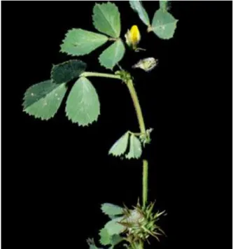
First studies on M. truncatula (Figure 1) as a model legume were related with its symbiotic relationship, Sinorhizobium meliloti in the early 1990s. Since that time, the spectrum of research in this model plant has evolved significantly as studies on root development, secondary metabolism, disease resistance, and ultimately to genomics, transcriptomics, proteomics, and metabolomics are being conducted.7,8

2

Medicago truncatula is an annual relative of

alfalfa (annual medic) with a genome size of about 500 Mbp, half of alfalfas. It has a diploid genome with 2n = 16 chromosomes, a short seed-to-seed generation time, susceptible of transformation, diverse mutant populations, large collections of diverse ecotypes and a good system for recombinant protein production.9

M. truncatula genomic sequence began at

the University of Oklahoma in 200110 and is now in the version 3.0 (10/10/2009 - www.medicago.org). Lotus japonicus was the

second legume species being sequenced. Both species have advanced rapidly over the past few years11-13 and since both are closely related, their genomic sequence along with predicted genes offer a great chance for plant comparative genomics. L. japonicus shares many of the same properties of M. truncatula. Therefore, also a lot of studies are made in this species. It could be a disadvantage to investigate two legume model plants as significant funds for each model plant would be needed. Instead, the parallel sequencing has shown to be an advantage because aspects of plant genome organization and evolution can be shown, among others. Moreover, a detailed comparison of these two model plants will improve the knowledge in a systematic and integrated way.14

In our study two lines of Medicago truncatula Gaertn cv. Jemalong were used: M9 and M9-10a. The latter is susceptible of being regenerated though somatic embryogenesis, according to methodologies developed in the Laboratory of Plant Cell Biotechnology at the ITQB/UNL, Oeiras, Portugal, and was obtained from the M9 genotype through somaclonal variation.15,16 Subsequently, an efficient protocol for transformation and regeneration by indirect SE was also successfully established. 17,18

1.2 Somatic Embryogenesis

Embryogenesis is a crucial process in the life cycle of plants spanning the transition from the fertilized egg to the generation of a mature embryo. In this process, the embryo acquires a

3

defined apical–basal pattern along the main body axis with shoot and root poles, a hypocotyl and cotyledons. Alternatively to the zygotic embryogenesis, somatic embryogenesis (SE) can also take place without need of gamete fusion (Figure 2). This process is possible due to the plants capability of cellular totipotency, where individual somatic cells can regenerate whole plants.19,20 SE is the developmental restructuring of somatic cells toward the embryogenic pathway. This way, somatic cells, in culture, are able to form complete embryos. The process throughout the somatic cells become embryogenic cells implies three major steps: induction, proliferation and differentiation. The first days are characterized by the induction of many stress-related genes leading some authors to think that SE could be an extreme stress response of cultured plant cells21. Many authors also conclude that the stress-response of cultured tissue could play a major role in somatic embryo induction.22-24 This step is usually acquired by direct stress stimulus or by the use of phytoregulators. Most embryogenesis cultures described in the literature require phytoregulators such as auxins and cytokinins but there are also phytoregulators free mediums to achieve the same response.22,25

After the first two to five days, the cells proliferate until we barely notice that at the beginning, we start with a leaflet. At this point we are in a presence of callus mass, a group of undifferentiated plant cells with

a less greenish colour. Starting around day fourteen we could notice pre embryogenic masses appearing. This is the beginning of the differentiation process, where we observe the pre-embryogenic masses turning into embryo in development. After five more days of culture, we will start seeing several embryos in a late globular/heart stage, that

Figure 2 – M9-10a leaflet callus with a somatic embryogenesis embryo (arrow).

Figure 3 – Example of BCV laboratory in vitro culture system. Several glass flask where both lines are grown. Each flask contains three plants.

4 each will lead to a new plant.

For in vitro culture (including SE), only a small amount of space is required (Figure 3), propagation is carried out under sterile conditions, and the rate of propagation is much greater than in macropropagation. Those characteristics make SE an important tool for the productivity of some commercial crops and a potential model system for the study of regulation of the earliest developmental events in the life of higher plants, namely the developmental mechanism of embryogenesis.26 These methodologies are also very commonly used as basis for cellular and genetic engineering, playing an important role in genetic transformation, commercial important metabolite production, somatic hybridization, somaclonal variation and more recently, plant stress studies.27-31

There are several works in the SE research. The majority of them on legumes are from M.

truncatula, probably due to the fact that it is a model plant as said in last section. In the

literature we could also found SE papers in Medicago sativa, Cajanus cajan, Lotus japonicus,

Glycine max, Vigna unguiculata, Arachis hypogaea and Astragalus melilotoides. Most of

them describe micropropagation methodologies to obtain somatic embryos and regenerate new plants but there are also papers reporting plant transformation32,33, characterization of genes34 or the identification of quantitative trait loci (QTL)35.

In M. truncatula, Imin N. et al. have conducted a genome-wide transcriptional analysis in another highly embryogenic Jemalong line 2HA, reporting differences in transcriptomes between that line and its non-embryogenic progenitor Jemalong at an early time point. The main differences were in carbon and flavonoid metabolism, phytohormone biosynthesis and signalling, cell to cell communication and gene regulation.36

Still, almost half a century of research in the SE area has passed by and knowledge on the acquisition of somatic embryogenesis is still in its infancy.37

1.3 Plant Proteomics

Over the past twenty five years, particularly in the last decade we have witnessed an increased effort to develop technologies that can identify and quantify large amounts of proteins in biological systems (cells or tissues, organs and ultimately whole organisms) in the hope of detecting disease and stress biomarkers, and mapping protein metabolic pathways, identify novel sites of phosphorylation among others. The complexity of a proteome led to the development of methods that aimed to a more efficient separation and increasing sensitivity in

5

detecting proteins.38 The latest advances in mass spectrometry (MS) provided significant improvements, such as sensitivity as well as speed and ease of detection.39,40 Still, MS techniques are frequently not able to characterize all the components in the complexity of a proteome. The analysis strategy, most of the time, involves temporarily limiting the number of proteins. With protein separation from a sample as a goal, science has used electrophoretic and chromatographic techniques, either separately or in combination. Although all these efforts lead to the separation and identification of thousands of proteins, no method can resolve all the proteins of a proteome, mainly due to the large number of different proteins and their different concentrations.41

Although used in particular circumstance, one dimensional separation is clearly inadequate to deal with complex protein mixtures such as those occurring in a variety of proteomic analysis. This was first recognized by Smithies and Poulik,42 which combined two electrophoretic processes in the same gel. This was the basis of many existing methodologies such as gel and capillary electrophoresis, and chromatographic.43

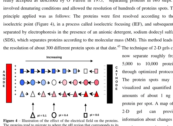
The technology of two dimensional polyacrylamide gel electrophoresis (2-D PAGE) was really accepted as described by O 'Farrell in 1975,44 separating proteins in two steps. It involved denaturing conditions and allowed the resolution of hundreds of proteins spots. The principle applied was as follows: The proteins were first resolved according to their isoelectric point (Figure 4), in a process called isoelectric focusing (IEF), and subsequently separated by electrophoresis in the presence of an anionic detergent, sodium dodecyl sulfate (SDS), which separates proteins according to the molecular mass (MM). This method leads to the resolution of about 300 different protein spots at that date.45 The technique of 2-D gels can now separate roughly from 5,000 to 10,000 proteins through optimized protocols. The protein spots may be visualized and quantified in amounts of about 1 ng of protein per spot. A map of a

2-D gel can provide

information about changes in protein expression level,

isoforms and

post-A N O D E + + + + + + + + + _ _ _ _ _ _ _ _ _ C A T H O D E Increasing pH pI = 8.6 pI = 6.4 pI = 5.1

Figure 4 – Illustration of the effect of the electrical field on the proteins. The proteins tend to migrate to where the pH region that corresponds to its pI, having no net charge. In blue the proteins are positively charged, travelling to the cathode. In red is the opposite, the proteins, negatively charged, travel to the anode.

6 translational modifications.46 In the field of plants, a large-scale study on the proteome of the

A. thaliana identified 2943 spots that were

derived from only 663 different genes.47 This is only a small number of genes, considering that more than 27,000 coding genes are provided in the genome sequence of A. thaliana.

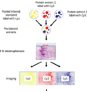
The latest method of protein visualization uses fluorescent markers and cyanine dyes (Figure 5). This method allowed a great advance in the technique of 2-D gels, especially in terms of comparing different samples as it is highly reproducible. In fact, if proteins from different experimental conditions were tagged with different cyanine dyes, it is then possible to run

both samples in one gel, avoiding the gel to gel variation. Fluorescent dye provide a great sensitivity, detecting about 125 pg of protein and providing a linear response to protein concentration of up to four orders of magnitude. However these dyes are more expensive than other techniques and require the use of expensive and sophisticated fluorescence scanner not frequently available in most plant research institutions.

After software analysis, gels are ready to be cut, choosing to be excised, spots of greatest interest to the matter under study. These will be submitted to an in gel digestion, typically with trypsin, so that the peptides generated can then be analyzed by MS and the protein identification inferred.

Proteomic studies, are also conducted in organisms with genomes not fully annotated,48 but have disadvantages in the treatment of data and the establishment of results with greater confidence. At present there are about ten fully sequenced genomes of plants (Arabidopsis

thaliana, Medicago truncatula, Glycine max, Oryza sativa, Vitis vinifera, Populus trichocarpa, citing some examples), others almost completed eg Lotus japonicus or Solanum lycopersicum. However, there are about 300,000 known species of terrestrial plants and the

plant model only represents a very small percentage of these. Even with the arrival of new model plants it will be difficult to reflect all the diversity of the plant kingdom.

Figure 5 – Example of a workflow scheme of the labelling of one sample with Cyanine dye in the DIGE technique. The protein samples and the IS run in the same gel throughout all electrophoretic process. Depending on each filter and excitation wavelength of the scanner, three different images are acquired and image analysis is ready to be performed.

7

1.4 Mass spectrometry

Mass spectrometry (MS) has become the analytical technology of choice for many aspects of proteomics analysis. MS provide direct information of the mass and the different structural modifications of a particular peptide, such as patterns of glycosylation, phosphorylation or other post-translational modifications by measuring mass changes. More detailed information could also be acquired by peptide fragmentation generating information of the peptide de

novo sequence. Mass spectrometry coupled to proteomics is extremely fast and can analyze

hundreds of samples sequentially from extremely small quantities of protein.

The proteins are huge cellular units. They need to be cleaved in small peptides in order to fit in the apparatus analysis range. As described before, trypsin is the most commonly used peptidase. Trypsin is an endopeptidase which cleaves the proteins in the region of the carboxylic residues of lysine or arginine. The distribution of these residues in the protein is in such a frequency that guarantees that the molecular weight of generated peptides is possible to be analyzed by the mass spectrometer.49

In the MS analysis, the sample requires a specific preparation. The Matrix-Assisted Laser Desorption Ionization (MALDI) method involves the formation of a gaseous phase by the use of excess matrix. Typically the matrix is composed by small organic molecules such as α-cyano-4-hydroxycinnamic acid or dihydrobenzoic acid, which co-crystallize with the molecules. After this step, samples are ready to go to MALDI apparatus and be submitted to subsequent ionization by nano-second laser pulses (Figure 6).50 In conjunction with the matrix, the peptides absorb light at a wavelength of the laser, ionizing and evaporating the molecules of the sample. This technique is common in studies to estimate the mass of the samples because it is versatile enough to analyze a large number of samples.51 The principle of Time-Of-Flight (TOF) analysers involves a separation based on time that the molecules take to travel a known distance. The ionized molecules are accelerated with the same kinetic energy and the velocity of the ions at the end is recorded in a detector, producing a spectrum. The mass of the protein peaks increases from left to right. The height of each peak is proportional to the number of ions that were on that particular ratio of mass / charge.

The spectrometers were improved when the tandem TOF apparatus appeared. The results of protein inference were improved and more trustable. Now we are able to generate much more information per peptide than before. The difference between MS and MS/MS is that after peptides generated with trypsin (see methods) were target and fragmented in ions like in MS, a precursor is selected in a mass analyzer and fragmented by collision with a gas (collision-induced dissociation). Afterwards its fragments are reaccelerated and travel until they reach

8

the detector. This will provide a set of new peaks specific for that precursor, that should be very similar to the one predicted by the in silico cuts, because the fragmentation occurs mainly in peptide bonds.40 It becomes easy to identify the major spot on a gel when matching to a specific database (our case), although it is directly dependent on the quality of the sequences. When using an organism protein database such as M. truncatula or A. thaliana this type of approach should be used. If the study organism doesn’t have a database with a high number of protein entries, still the MS technique could be used for several different analyses (despite less specific) or the MS/MS results could be submitted to a larger protein database or even sequenced de novo and submitted to a blast search. MALDI TOF-TOF is the apparatus used in this work. This type of technique is being routinely used in biological mass spectrometry. Although not directly related to electrophoresis or 2-D gels, mass spectrometry is indeed a fundamental tool in any work of proteomics analysis.

Figure 6 – View from outside (left) of the MALDI TOF-TOF 4800 apparatus and a scheme of the major components (right).

9

1.5 Aim of this project

About ten years ago, a highly embryogenic line of Medicago truncatula (M9-10a) was derived from a non-embryogenic line (M9) of the Jemalong cultivar. This work was conducted in the Plant Cell Biotechnology Laboratory (ITQB/UNL, Portugal), as described in Neves et al. (1999) and in Santos and Fevereiro (2002).15,16 These two lines could be considered an ideal to be used in the study of SE process as they share an extremely similar genetic background, differing essentially at the level of the SE ability. The aim of this project is to analyze differentially expressed proteins in two lines of M. truncatula, the non-embryogenic (M9) and the non-embryogenic one (M9-10a) in order to further understand the process of embryogenesis. Since we already knew the time course of the shift in embryogenic development, we choose the time points thought to be the most critical. Using a combination of two-dimensional electrophoresis and protein identification by mass spectrometry we analyze the proteome of the lines according to those time points, 0, 2, 5, 14 and 21 days.

The long term goals for this project is to be able to identify regulatory and metabolic pathways (such as hormone activation, wounding, cell division or differentiation) and place them in the somatic embryogenesis overall view. Pathway identification can for example lead to a suggestion on how to improve the somatic embryogenenis accomplishment in plants that does not have those characteristics and are hard to genetic engineer. Results obtained are likely to be extrapolated to other legume species of economic importance, therefore of relevance to the genetic improvement of these crops and consequently, to world agriculture.

10

2. Results

2.1 Trial with coomassie staining

Since we were aiming to obtain the new cells that were growing after the wounding of leaflets and this was carefully conducted using macroscopic lenses, we had to avoid tissue oxidation and protein cleavage (Figure 7). We had used a simple sucrose-tris-DTT solution at 4ºC and extract the tissue directly. In the statistical analysis we didn’t have the majority of high molecular mass proteins down regulated and the small MM proteins up regulated, showing that we avoided protein cleavage and also the tissue didn’t show signs of oxidation. With this new buffer we wanted to assure that the protein precipitation using cold acetone would still be a good extraction method. For that we collected the tissue to the medium and macerated the plant material in liquid nitrogen and try to precipitate the material in microcentrifuge tubes with cold acetone. Samples were run in a 1-D gel and show interfering compounds in the low molecular mass part of the gel. With that we have try to minimize the sucrose interference. After

tissue collection was done, the excess of buffer was removed and were samples frozen. We also had the opportunity to use an homogenizer to grind reproducibly the tissues and we incorporated an intermediate washing step with ammonium acetate in methanol. With those modifications the resolution did improve significantly and we could start testing for IEF.

For the IEF we first tried to run the samples at 7 cm strips with protein loading being done passively. The first part of an IEF run usually corresponds to low voltage steps. The time spent on this low voltage periods is important because it is in this step that some interfering compounds such as salts or other molecules are removed. Salts, as example, would give a high conductivity and therefore interfering in protein focussing, until they reach the edge of the strip.

From a few protocols we have chosen the protocol with one cleaning hour and two and a half focusing hour. From this point we have tried to adapt it to a similar one able to run 24 cm strips with 400 µg of proteins and now with six hours for the cleaning part and fourteen for the protein focusing. The gel performance was considered reasonable to continue (Annex figure I), so we have progressed our work with the protein labelling with cyanine dyes, the DIGE technique as described below.

Figure 7 – Example of the sample isolated parts in the buffer.

11

2.2 Differentially expressed proteins

After the optimization of the extracting methods and good focusing in 24 cm strips we went further on with proteomic analysis. Before we ran our batch of fifteen gels, we wanted to see if the samples were ready to be labelled. The pH of each sample is one important aspect of labelling, being pH 8.5 the optimal and pH below 8.0 or above 9.0 not suitable for it. Even though the measurements of the pH were done by pH strips, and this could lead to miss interpretation, the trial gel with two samples and one internal standard showed that the samples were correctly labelled and well focussed.

The same procedures of the trial were used in the analysis gel. Differently from the optimization runs’ the proteins were now loaded by the cup loading method. In the IEF of all the analysis gels, the current never reach the limit of 50 µA and then, never limiting the voltage. This is a parameter that would help to evaluate the consistence of the protein focussing.

The beginning of analysis with the Progenesis SameSpots (Nonlinear Dynamics) software revealed about 1300 individual spots. From this total of proteins, several groups were made in order to do the Anova statistic analysis. For spot picking we have chose the sum of proteins differentially expressed in each time point for both plant lines and for each line along the time, giving a total of 545 protein spots. Since it would have been almost impossible to identify all of them in such a short time, a total of 174 proteins were selected to the tryptic digestion and consequent identification. About 43% of the spots had a significant hit. In here we present the tables of the differentially expressed proteins for each time point with the identification, if we had a match (see methods).

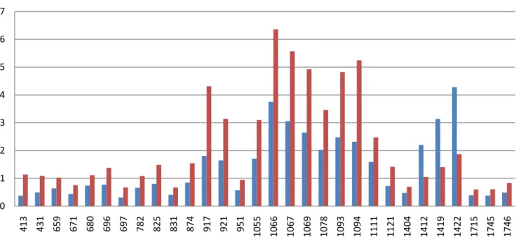
In Table 1 we could see the SameSpots attributed number for each spot, the correspondent p value (significance) and protein fold change. In the last column (Average Normalized Volumes) both values, M9 and M9-10a gave the value to the correspondent chart (Figure 8).

From this data we were able to understand that the plant lines had some proteome differences even before the leaflets being induced to somatic embryogenesis medium. There were thirty proteins differentially expressed and we were able to identify about half of them. The most different identified spots were 917, 921, 1093, 1078, being more expressed in the embryogenic line (M9-10a) and 1419, 1422 being more expressed on the non-embryogenic one (M9).

At day two we had identified two differentially expressed proteins from a total of six (Table 2). Only one was more expressed in M9-10a (358) and all the other were more abundant in

12

Table 1 – Spots showing statistical significance differences between the two lines, M9 and M9-10a at Day 0. Identified spots are marked in red.

Spot Anova (p) Fold

Average Normalised Volumes M9 M9-10a 413 0,01 3 0,383 1,136 431 0,017 2,2 0,495 1,088 659 0,012 1,6 0,645 1,024 671 0,014 1,7 0,441 0,755 680 0,015 1,5 0,74 1,117 696 0,013 1,8 0,776 1,377 697 0,014 2,1 0,315 0,672 782 0,01 1,6 0,661 1,082 825 0,006 1,8 0,805 1,487 831 0,002 1,7 0,406 0,671 874 0,002 1,8 0,848 1,548 917 0,016 2,4 1,807 4,316 921 0,019 1,9 1,647 3,139 951 0,013 1,7 0,571 0,947 1055 0,011 1,8 1,709 3,099 1066 0,009 1,7 3,755 6,359 1067 0,005 1,8 3,058 5,571 1069 0,012 1,9 2,645 4,928 1078 0,017 1,7 2,025 3,461 1093 0,012 1,9 2,476 4,825 1094 0,012 2,3 2,316 5,245 1111 0,019 1,6 1,593 2,476 1121 0,006 2 0,724 1,418 1404 0,019 1,5 0,476 0,699 1412 0,004 2,1 2,201 1,051 1419 0,003 2,2 3,138 1,406 1422 0,019 2,3 4,28 1,871 1715 0,011 1,5 0,396 0,599 1745 0,012 1,6 0,382 0,608 1746 0,002 1,7 0,489 0,835

Table 2 – Spots showing statistical significance differences between the two lines, M9 and M9-10a at Day 2. Identified spots are marked in red.

Spot Anova (p) Fold

Average Normalised Volumes M9 M9-10a 358 0,015 2,1 0,671 1,441 709 0,003 2,7 0,984 0,369 1120 0,013 1,5 2,531 1,716 1228 0,017 2 2,789 1,375 1356 0,011 1,8 1,883 1,034 1701 0,007 1,6 0,55 0,334

Table 3 – Spots showing statistical significance differences between the two lines, M9 and M9-10a at Day 5.

Spot Anova (p) Fold

Average Normalised Volumes M9 M9-10a 384 0,013 1,8 1,034 1,813 1088 0,002 1,6 1,034 1,632 1716 0,000381 1,7 0,881 1,481

13 0 1 2 3 4 5 6 7 413 431 659 671 680 696 697 782 825 831 874 917 921 951 _{1055 1066 1067 1069 1078 1093 1094 1111 1121 1404 1412 1419 1422 1715 1745 1746}

Day 0

Day 2

Day 5

Figure 8 – Graphical representation of the averaged Normalised Volumes for Day 0.

Figure 9 - Graphical representation of the averaged Normalised Volumes for Day 2.

Figure 10 - Graphical representation of the averaged Normalised Volumes for Day 5.

14

Table 4 – Spots showing statistical significance differences between the two lines, M9 and M9-10a at Day 14. Identified spots are marked in red.

Spot Anova (p) Fold

Average Normalised Volumes M9 M9-10a 222 0,018 1,6 1,082 0,696 261 0,015 1,8 1,24 0,684 387 0,008 2,3 1,313 0,561 913 0,018 1,8 0,917 0,5 916 0,014 1,8 1,344 0,736 927 0,012 2,5 0,77 1,912 972 0,007 4,1 2,582 0,637 990 0,018 3,8 2,48 0,661 1000 0,006 1,8 0,973 1,73 1106 0,007 1,9 0,688 1,309 1111 0,003 2,1 1,665 0,78 1140 0,005 1,9 1,535 0,813 1281 0,002 1,9 0,866 1,644 1290 0,018 2,7 1,59 4,306 1312 0,002 1,7 0,978 1,666 1322 0,000867 1,7 0,857 1,472 1348 0,000225 2,8 1,094 3,064 1359 0,005 1,6 1,429 2,226 1363 0,014 2,9 0,868 2,525 1366 0,000201 3,1 1,067 3,346 1371 0,002 1,7 0,881 1,537 1397 0,00100 2,5 1,13 2,775 1399 0,000496 2,8 0,976 2,732 1409 0,009 2,1 0,532 1,101 1411 0,009 2,6 0,84 2,159 1450 0,013 2,4 0,477 1,129 1469 0,011 3 0,617 1,836 1502 0,007 1,7 0,942 1,622 1527 0,012 2,7 0,643 1,705 1702 0,019 1,9 1,261 2,391

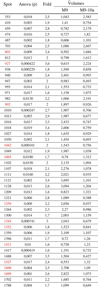
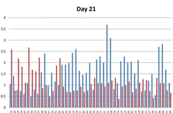
Table 5 – Spots showing statistical significance differences between the two lines, M9 and M9-10a at Day 21. Identified spots are marked in red.

Spot Anova (p) Fold

Average Normalised Volumes M9 M9-10a 353 0,018 2,5 1,043 2,583 410 0,003 1,9 1,41 0,754 459 0,007 2,8 0,782 2,179 474 0,016 2,5 0,727 1,82 487 0,002 1,8 0,606 1,101 703 0,004 2,5 1,086 2,667 803 0,009 3,4 0,502 1,684 812 0,012 2 0,798 1,612 927 0,000422 3,6 0,615 2,224 938 0,000229 1,8 1,569 0,858 940 0,009 2,4 2,401 0,993 947 0,003 2 0,983 0,493 955 0,014 2,1 1,553 0,733 971 0,017 1,6 1,158 1,875 982 0,0130 2,2 1,006 2,191 992 0,017 2 1,897 0,926 1010 0,000247 2,7 1,907 0,706 1013 0,003 2,9 1,987 0,677 1016 0,017 3,3 2,433 0,747 1018 0,019 3,4 2,606 0,759 1027 0,014 1,8 1,635 0,929 1030 0,002 2,1 1,454 0,693 1042 0,000101 2 1,543 0,756 1049 0,012 1,9 1,987 1,038 1065 0,0180 1,7 0,78 1,312 1102 0,0150 2 2,135 1,094 1107 0,018 2,1 2,276 1,078 1111 0,0160 2,2 2,021 0,935 1121 0,002 3,4 3,695 1,101 1128 0,013 2,6 3,094 1,204 1209 0,012 1,6 0,823 1,321 1221 0,006 2,8 1,089 0,388 1259 0,009 2,2 2,056 0,937 1264 0,002 2,3 2,27 0,986 1300 0,014 1,7 2,003 1,159 1345 0,000741 3 2,043 0,679 1352 0,006 1,8 1,523 0,841 1359 0,006 1,9 2,109 1,107 1396 0,011 1,7 0,72 1,26 1411 0,01 1,6 0,758 1,23 1417 0,000419 1,6 1,191 0,732 1488 0,007 3,5 1,504 0,427 1527 0,017 2,4 0,553 1,32 1698 0,004 2,5 2,708 1,09 1699 0,001 2,6 2,822 1,073 1702 0,011 2,2 1,685 0,764 1788 0,004 1,7 1,099 0,649

15 0 0,5 1 1,5 2 2,5 3 3,5 4 353 410 459 474 487 703 803 812 927 938 940 947 955 971 982 992 _{1010 1013 1016 1018 1027 1030 1042 1049 1065 1102 1107 1111 1121 1128 1209 1221 1259 1264 1300 1345 1352 1359 1396 1411 1417 1488 1527 1698 1699 1702 1788}

Day 21

Day 14

Figure 11 - Graphical representation of the averaged Normalised Volumes for Day 14

16

the non-embryogenic lines (Figure 9). In the next time point, samples in induction medium for five days, we weren’t able to identify differentially expressed proteins, although there were three differentially expressed proteins all of them more abundant in M9-10a (Table 3 and Figure 10). At the fourteen days stage we expect the beginning of cellular reorganization. In this time point the majority of proteins identified were again more expressed in the embryogenic line (Table 4). The biggest differences in protein accumulation were in spot 927, 1290, 1348, 1363, 1366, 1397, 1399, 1411, 1469 and 1527 (Figure 11). These spots were more had more protein accumulation in M9-10a with fold changes from 2.5 to 3.1. All of them were identified except 1397 and 1399. The spots 387, 972, 990 and 1111 were more present in M9, with fold changes from 2.1 to 4.1, unfortunately none of these were identified.

At last, after twenty one days of the leaflets placed on induction medium, we identified twelve differentially expressed proteins (Table 5) from a total of forty seven. Five of them being more present in M9-10a line, 803, 927, 1065, 1411 and 1527, with fold changes of 3.4 and 3.6 for the first two, (respectively) and 2.4 for the last one. The others were more abundant in M9 with a maximum of 3 fold change for spot 1345 (Figure 12).

We also tried to look at our data with a different point of view, in the embryogenic development point of view. In order to do that we have also compared the different time points in each plant along with the time and try to relate those proteins with the embryogenesis stage. If we look at the Annex figure III, from a total of sixty four differentially expressed proteins in M9 and two hundred and twenty two in M9-10a, we barely could notice what expression patterns are occurring. Consequently, to compare our proteins, we have chosen just the identified proteins and split them in two groups, the ones that seem to be present in the initial stages and absent at the end or vice versa. From what we observe, a lot of proteins have similar pattern, both in M9 and M9-10.

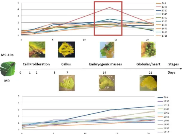
With less frequency we could see that, from our identified proteins, just two of them have different patterns in the different lines according to our grouping (992 and 1411). Also there are some proteins that are present just in one of the plant lines, two in the M9 line, being up regulated and several in M9-10a both up and down regulated (Annex figure IV). What we have notice is that there are at least one specific pattern of protein expression that seem to be characteristic of the embryogenic line. After drawing the proteins common in both lines being up regulated to each other, we could see that at fourteen days of culture, there are several proteins that seem to have an expression peak at that time point. This is the time point where the pro-embryogenic masses are visible in our tissues, point to the probable importance of those proteins in the development of the embryo (Figure 13).

17

In the principal component analysis (PCA), where the spots of each gel are combined in one single spot, we can see that each set of biological replica group together. This is consistent with the significance of the analysis, where the differences that we observe in each spot are not random but driven by experimental conditions (Annex figure V).

The ratio of the identification of proteins was not as high as we expected. In sequenced organism usually the identification rates are above 65%. Even thought we had used a combined search in multiple databases our identification ratio was lower than expected. A major factor for this was probably an excessive amount of spots sent to be cut, being the usage of the spot picker compromised. The table of identification is reported on the annex section, in the Annex table I as well as the image of our picking gel after the extraction with the spot picker (Annex figure VI).

Figure 13 – Comparison of the expression of the same differentially expressed proteins in both lines. In the red square we highlight the peak of expression that is characteristic of the embryogenic line.

18

3. Discussion

3.1 Trial with coomassie staining

Sample extraction on proteomic works is an important subject. One of the many reasons of

the poor reproducibility of 2D-gels is sample handling, mainly between experiments in different labs.52,53 In order to avoid protease degradation,

the majority of protein extraction protocols demand a rapid sample disruption and protein denaturation using TCA or SDS or urea. However, depending on the extraction method used, a different fraction of the proteome could be obtained.54 In order to avoid fading the differences in the differentially expressed protein, we tried to recover as much as possible the new cells in division after wounding (Figure 14). By doing so,

we hoped to get rid of most of the leaf ordinary metabolic proteins.

Our extraction methodology was a regular precipitation protocol with TCA and acetone with some adaptation in the washing steps from Wang et al. protocol.55 The combination of the homogenizer and the washing solution (see methods) had proved to be a good add-on to our extraction methodology. The homogenizer brought considerable advantage in terms of speed, protein extraction yield and reproducibility, and the washing steps helped us to get rid of interfering compounds (Figure 15).

After confirming that the IEF protocol was resolving efficiently the proteins, we continued throughout the next step, the protein labelling with cydyes. In the annex we present an image of the DIGE gel used as reference for the alignment (Annex figure II). This image is clearly better than the one of the last coomassie gel (Annex figure I). The coomassie image doesn´t look as good as our DIGE gels but it should be taken in consideration the sensibility of the staining and the quality of the image acquisition. Even though the image of coomassie gel

Figure 14 – Examples of the section isolated from M9-10a after 5days in induction medium. The cuts were performed with a scaffold in a macroscopic lens.

Figure 15 – In A we have a 1D-gel from samples ready to use in DIGE and B is a 1D-gel before using homogenizer and washing steps.

19

shows that we were successful in the application of the IEF program and extraction buffer, having a good focusing in low contaminants.

3.2 Differentially expressed proteins

Somatic embryogenesis in the M9-10a genotype of M. truncatula was first described in Santos et al. and a global scheme of the all process, in comparison with M9, is shown in Figure 16.16 During

the initial phases of

embryogenesis, somatic cells progress through a series of events referred usually induction, competence acquisition and differentiation.

In the first days we could

observe some new cells,

proliferating in the wounding

zones. These cells keep

continuously multiplying leading to a formation of a callus, normally at fourteen days. The callus stage is where we could barely notice that cell masses originate from leaflets. From that time point, the embryonic masses begin a differentiation process where we could see rounded green masses coming out from the callus. Those masses will give origin to the embryos (globular and heart shaped) in about twenty one days after the beginning of the culture. On the other hand, even though the initial phases of M9 explants are quite similar to the embryogenic line,

Figure 16 – Figure comparing each line to each other when the samples were collected. Arrows point to the pro-embryogenic masses at 14 days and developing embryos in 21 days (M9-10a).

20

as days pass by, will maintain a callus stage. Also we can notice that the size of the callus are smaller and the leaflets cells become yellow and eventually die. Despite the M9-10a is derived from the M9 line in this and in previous experiments it has never proceeded to the next embryonic step.

The difference in the proteome before explants placed in induction medium revealed that a

priori we weren’t starting with exactly the same plants. From the proteins referred on the

results we highlight 917, an RNA-binding region RNP-1 (RNA recognition motif) and a low molecular mass spot, 1419, identified as ubiquitin extension protein.

RNA-binding proteins are cellular proteins that regulate gene expression principally at the post-transcriptional level, which involves pre-mRNA splicing, nucleocytoplasmic mRNA transport, mRNA stability and decay, and translation.39, 40 They could be characterized by the presence of several conserved motifs and domains, including the RNA-recognition motif (RRM), glycine-rich domain, K homology domain, RGG-box, and zinc-finger motif 58,59. Despite being a bit vague this could point a major factor in the difference between both lines. The somaclonal variation that could have happened when the M9-10a was generated could lead to different gene regulation as mentioned above. Also the presence of a high level of ubiquitin in the M9 line could be an indicator that some proteins important to the induction of the embryogenic process aren´t being accumulated in the cell. The covalent attachment of ubiquitin to a substrate protein changes its fate. Proteins typically tagged polyubiquitin chain (several ubiquitin residues) become substrates for degradation by proteosome units.60

At days 2 and 5 we could observe that the differences in proteins between lines become shorter. At day 2, we just have six different proteins and this count drops to three different proteins expressed at day 5. This can point to two different situations: either we could have the tissues become equal at the protein level, and the differences for the embryogenic process are happening in other time points; or the differences in protein expression in this time point are crucial for the embryogenesis process. With the identification of the remaining proteins, we hope to achieve the answer to our question. In the latest time points we begin seeing more proteins being at M9-10a, consistent with the fact that the tissue is on a differentiation process but later, at twenty one days, is the M9 line that has larger expression of the majority of proteins. Since the M9 callus in the last time points is turning yellow and it will eventually die, upon a wider overview, we believe that the majority of the proteins with greater amount is justified by cellular senescence.

21

Regarding a continuing time overview with the identified proteins (Annex figure IV) we could see that we have several proteins following the same pattern along the time (Figure 13 – Comparison of the expression of the same differentially expressed proteins in both lines.black spot numbers), some exclusive differentially expressed proteins in each line for (red spots numbers) and another one following different patterns in each line (blue spots numbers). In Figure 17 we could see that the majority of the proteins that had similar patterns were proteins related to stress response. This major number appears probably due the fact that in vitro culture is not a natural condition in the M. truncatula. Also we have noticed two big groups related with the cells in continuous proliferation and also with the differentiation step (cellular component organization and developmental process).

For another example of how interesting this approach could be, we will focus on the blue spot 1411 (Figure 18),

identified as nucleoside

diphosphate kinase

(NDPKs). These are thought to be involved in processes such as control of cell proliferation56 and oxidative stress tolerance44,45 or hormone response.63,64 The chart of protein expression

Figure 17 - Pie chart generate by blast2go software. The represented biological process groups contain the proteins that on the time evaluation comparison have showed the similar expression pattern (black spots)

Figure 18 - Chart comparing the expression profiling of the nucleoside diphosphate kinase (1411), in both lines, M9 and M9-10a.

Response to abiotic stimulus 9% Translation 13% Catabolic process 9% Signal transduction 9% Cellular component organization 13% Developmental process 13% Response to biotic stimulus 9% Response to stress 25%

Biological Process

22 on both lines shows that usually the M9 line has a bigger amount of this protein but as days pass by in the induction medium, the accumulation keeps a residual level. On the other hand, M9-10a has a lower accumulation on its leaflets but after a few days in culture, protein accumulation increases. The peak of accumulation coincides with the formation of embryogenic masses and then it returns to its basal level. This could

be one major factor of what is illustrated in Figure 19. The phenomena looks like an accumulation of anthocyanines also know to be related with oxidative stress tolerance.65 NDPK protein could be up regulating this pathway or being regulated along with this pathway. Citing two more proteins with similar pattern in M9-10a, we have 1290 and 1699, identified as PAP fibrillin and transposase, respectively. PAP fibrillins (Figure 20), also named as plastoglobulins, have a predominantly structural role, possibly regulating size and shape of lipoprotein structures in plastids.66 They had been described as being up regulated in pathways linked to the cellular redox state, participating in structural stabilization of thylakoids upon environmental constraints and preventing damage resulting from osmotic or oxidative stress.67 If so, it could also be involved in the above mentioned phenomena.

Regarding the transposases (Figure 21), their function is to move double-stranded DNA directly by excision and insertion and they are sometimes associated with insertion sequences, but often just catalyze their own mobilization. They were described as possibly essential for plant growth and development as when a transposase sequence in Arabidopsis was

Figure 19 - Image of the concentration of the pigment molecules at day 14. 0 1 2 3 4 5 0 5 10 15 20 M9-10a M9 0 1 2 3 4 5 0 5 10 15 20 M9-10a M9

Figure 20 - Chart comparing the expression profiling of the PAP fibrillin (1290), in both lines, M9 and M9-10a.

Figure 21 - Chart comparing the expression profiling of the Transposase (1699), in both lines, M9 and M9-10a.

23

interrupted, seedlings grew very slowly, and showed no expansion of the cotyledons or development of normal leaves.68 The increasing expression in the M9 line of this protein could also be related with the probable cause of the M9-10a throughout somaclonal variation. Some authors have described the relation between this protein and the somaclonal variation process, which is boosted by the use of in vitro culture system.69,70 Plant transposons appears to be regulated by DNA methylation. A correlation between increased DNA methylation and plant transposon inactivity has been described for several transposon families in maize and other plants.71,72

A deeper evaluation would then need to be done. In fact, there are several proteins that have the peak of expression at day fourteen. In the software analysis we have used a dendrogram to sort them out (Figure 22). From the total of two hundred and twenty two proteins, eighty are marked in red.

Closing this section with a method evaluation, we could say that the electrophoresis technique using the cyanine dye labelling has proved to be an excellent tool to compare our different plant lines. The protein identification in further works should be optimized. The use of spot picker in proteomics works is commonly known for being high throughput, since in one hour we could have up to five hundred spots; less exposed to contaminants, mainly due to the fact that the cutting is done in a closed environment; more precise, because it is the analysis software that generates a coordinate list that the spot picker interpret itself. Our major problems in the use of this apparatus were the difficulty in the loading of the coordinate list and “excess throughput” for one single gel. Since the ExQuest (Bio-Rad) spot cutter isn’t fully compatible with our analysis software, we had to generate a generic coordinate list that later on needed to be fitted in the right spots. This generates some loss of precision due to human manipulation. In the future some precise reference coordinates should be used in this

Figure 22 – Dendrogram generated by SameSpots in the M9-10a analysis along the 21 days of culture. Each blue mark at distance 0 corresponds to a differential expressed protein. The red clade is marking the group of proteins that have an expression peak at day 14.

24

system. Also a less number of spots to be taken per gel should be taken in account. In some spots, the surrounding excision area, have been damaged. If two spots were really close to each other, the second one would probably not be taken. With those improvements we are expecting to have better results than when performing manual picking.

25

4. Conclusions and future prospects

We were able to mount an efficient system in order to collect meticulously our sample material. We have shown that the DIGE technique is a very sensible approach, leading to a huge amount of information. In order to reach its potential, extraction and focusing of the samples must have a careful attention. In this work we were able to optimize both steps and successfully label our samples detecting a total of 1300 individual spots. From these, 540 spots were chosen for gel picking as they were differentially expressed in any time point. Some of the more interesting spots were chosen to be firstly identified, summing 174 spots. A total of 73 differential protein spots were identified by the mass spectrometer apparatus MALDI TOF-TOF and with the continuation of our work, we expect to identify several more. The protein profile of M9-10a has shown interesting patterns, with several proteins having an expression peak around day fourteen. This coincides with the formation of the pro-embryogenic masses that will lead to embryo formation. Some proteins have been highlighted and their probable role in the somatic embryogenesis discussed. With the identification of the majority of the others, we hope to find ourselves in position to describe more extensively some pathways related with the embryogenic response, and in that way, enlighten the process of somatic embryogenesis in plants and contribute to the improvement of legume plant species and simultaneously of human and animal nutrition.

26

5. Material and Methods

5.1. Plants

Embryogenic (M9-10a) and non-embryogenic (M9) lines of Medicago truncatula Gaertn cv. Jemalong were used.15 Both lines were maintained under in vitro culture in MS (Murashige and Skoog) medium, including minerals and vitamins (Duchefa Biochemie) with 30 g L-1 sucrose. pH was adjusted to 5.85 and the medium solidified with 7 g L-1 micro agar. Plant cultures were transferred to fresh medium monthly and maintained in a growth chamber (Phytotron EDPA 700, Aralab) under 16h photoperiod of 100 μmol m−2 s−1 applied as cool white fluorescent light and halogen light. The day/night temperature was 24ºC/22ºC.

Calli was induced from well-expanded leaflets. Leaflets were placed onto a wet sterile filter

paper in a Petri dish to prevent excessive desiccation and wounded perpendicularly to the central vein using a scalpel blade. The wounded explants were transferred to EIM (embryogenic induction medium), MS basal medium with 30 g L-1 sucrose, pH 5.85, 0.4 μM 2,4-dichlorophenoxyacetic acid (2,4-D), 0.9 μM zeatin, solidified with 2 g L-1 gelrite. Embryogenic calli cultures were maintained in the same growth chamber as plant lines. Samples were collected from leaflets at five time points after placing the folioles in EIM: 0, 2, 5, 14 and 21 days.

5.2. Protein extraction

Plant material was collected to a solution of 100mM Tris-HCl pH 8.0, 10mM DTT, 30% Sucrose, and kept at -80ºC until the extraction was performed. The plant material was emerged in N2 and grinded with a Mikro-Dismembrator S (Sartorius) at 3.000 rpm for 90

seconds. Proteins were precipitated with a solution of 60 mM DTT, 10 % TCA in Acetone (w/v) cooled at -20ºC and incubated for 1 hour at -20ºC for later 15 seconds vortex and a 16,000g, 10 minutes, at 4ºC centrifugation. The pellet was first washed in 100 mM ammonium acetate in methanol cooled at -20ºC and then in 80 % acetone cooled at -20ºC. Between each washes, pellet was incubated at -20ºC for 30 min, afterwards 15 seconds vortex and 16,000g, 10 minutes at 4ºC centrifugation. The pellets dried for 1 hour in a Thermomixer (Eppendorf) at 800 rpm, at room temperature (RT) and then were dissolved in IEF DIGE lysis

27

(buffer 30 mM Tris, 7 M Urea, 2 M Thiourea, 4% (w/v) CHAPS, pH 8.5) for 2D gel electrophoresis.

5.3. Two-dimensional gel electrophoresis

5.3.1. Preparative gels

Samples were completely dried from the acetone and then thoroughly dissolved in 200 µL of DIGE lysis buffer at RT in a Thermomixer (Eppendorf) at 1,000 rpm for 4 hours. Samples were then centrifuged at 20,000g for 30 min at RT and supernatant collected to new tubes. The protein concentration was determined with 2-D Quant Kit following manufacturer’s instructions (GE Healthcare) and results were subsequently confirmed with 1D gel. Rehydration loading was performed with 450 μl solution, consisting of 400 μg proteins, DeStreak Rehydration Solution (GE Healthcare) to a final volume of 450 μl, and 0.5% IPG buffer (pH 3-11, GE Healthcare).

The staining method used was Colloidal Coomassie Brilliant Blue, where firstly the proteins were fixed (50 % Ethanol (v/v) and 2.55 % phosphoric acid (v/v)) for 18 h. Afterwards the gels were pre-incubated (34 % methanol (v/v), 2.55 % phosphoric acid (v/v) and 17 % ammonium sulphate (w/v)) for 1 h and then incubated with Coomassie Brilliant Blue (350 mg Coomassie Brilliant Blue (G-250) per litre), staining for 100 h. Subsequently, gel was washed three times in 500 mL double distilled water to remove background stain and was left in water for 20 h. For testing the sample extraction and the IEF methods both 7cm and 24cm IEF strips were used.

5.3.2. Differential gel electrophoresis (DIGE)

The pH of each sample was adjusted to 8.5 with 100 mM and 250 mM NaOH solution in the day when labelling would be performed. An internal standard was made by mixing 15 μg of each of the samples used in the study. The samples (30 μg) and the internal standard were labelled with CyDye DIGE Fluor minimal dyes (240 pmol per 30 μg protein, GE Healthcare) and incubated on ice for 30 min in the dark. One microlitter of 10 mM Lysine was then added to stop the reaction, and the samples were left on ice for 10 min in the dark. Replicates were