Atlas jet trigger: performance and in-situ calibration studies

(1)

DEPARTAMENTO DE F´ISICA

ATLAS JET TRIGGER:

PERFORMANCE AND

IN-SITU CALIBRATION

STUDIES

Joana Machado Migu´

ens

MESTRADO EM F´ISICA

( ´Area de Especializa¸c˜ao em F´ısica Nuclear e Part´ıculas)

(2)

(3)

DEPARTAMENTO DE F´ISICA

ATLAS JET TRIGGER:

PERFORMANCE AND

IN-SITU CALIBRATION

STUDIES

Joana Machado Migu´

ens

MESTRADO EM F´ISICA

( ´Area de Especializa¸c˜ao em F´ısica Nuclear e Part´ıculas)

Disserta¸cão orientada por: Professora Doutora Amélia Maio Co-orientada por: Doutora Patricia Conde Mu´ıño

(4)

(5)

The LHC at CERN will provide collisions of proton beams with a pioneer en-ergy of 14TeV and an unprecedented luminosity of 1034_cm−2_s−1_{, extending}

the frontiers of Particle Physics.

ATLAS is a general-purpose detector, designed to cover the widest range of physics possible by analyzing the myriad of particles produced by the LHC.

Collision data from the LHC will be delivered to ATLAS at an unsus-tainable rate of 40MHz. Working in three steps, the ATLAS trigger system will effectively reject uninteresting events, still maintaining an excellent and unbiased efficiency for rare signals, in order to reduce the input rate to a manageable 200Hz.

Hadronic jets will be among the most commonly produced objects at the LHC. They will represent, at the same time, signatures for many physics processes and background for nearly every physics analysis. Thus, the per-formance of the trigger system depends heavily on its ability to reconstruct jets. Moreover, precise jet reconstruction cannot be achieved without energy calibration, which is why the energy of trigger jet is calibrated at Level-2.

The work presented in this thesis was developed in two steps.

First, the performance of the ATLAS jet trigger system was evaluated using data from cosmic muon runs. This was done by comparing the prop-erties of the jets reconstructed by the trigger and reconstructed offline. The analysis was simple but, nonetheless, powerful, since it allowed the identifi-cation of noisy cells and calibration problems.

For the second study, a in-situ calibration method was applied to Mon-teCarlo simulated jets to evaluate if the method can be used with real colli-sion data to validate and tune the calibration applied to Level-2 trigger jets.

(6)

The method, named intercalibration in η, proved capable of improving the Level-2 jet energy scale up to an uncertainty of 1% for jets with transverse momenta above 1TeV. Furthermore, the analysis strongly suggests that the method can be used with real data for the same purposes.

Keywords: CERN, LHC, ATLAS, hadronic jets, trigger, in-situ calibra-tion.

(7)

O LHC no CERN vai provocar colisões de feixes de protões em condi¸cões sem precedentes - energia de 14TeV e luminosidade de 1034_cm−2_s−1 _{- alargando}

as fronteiras da F´ısica de Part´ıculas

ATLAS é um detector de carácter genérico, concebido para identificar a m´ıriade de particulas produzidas no LHC, cobrindo um vasto leque de processos de f´ısica.

ATLAS receberá dados das colisões no LHC a uma taxa insustentável de 40MHz. O sistema de trigger de ATLAS actua em três n´ıveis para rejeitar eventos, mantendo-se eficaz na deteçcão de processos de f´ısica interessantes e de sinais raros, reduzindo a taxa para 200Hz.

No LHC os jactos hadrónicos serão dos objectos produzidos em maior abundância. Para ATLAS, os jactos são, por um lado, assinaturas de pro-cessos f´ısicos relevantes e, por outro, fundo para a maior parte das análises de f´ısica. Assim, o desempenho do sistema de trigger depende fortemente da sua capacidade de reconstruir jactos. Para além disso, uma reconstru¸cão precisa requer calibra¸cão da energia dos jactos, que a n´ıvel do trigger é efectuada no Level-2.

O trabalho apresentado nesta tese foi desenvolvido em duas partes. Primeiro, o desempenho do trigger de jactos de ATLAS foi avaliado com dados de runs de muões cósmicos. A avalia¸cão foi feita comparando as propriedades dos jactos reconstru´ıdos pelo trigger e reconstru´ıdos offline. Apesar de simples, a análise mostrou-se poderosa, permitindo a identifica¸cão de células ruidosas e problemas de calibra¸cão do detector.

Para o segundo estudo, aplicou-se um método de calibra¸cão in-situ a jactos simulados de MonteCarlo, por forma a determinar se o método pode ser utilizado com dados reais de colisões para validar e afinar a calibra¸cão

(8)

aplicada aos jactos do Level-2 do trigger. Com este método, designado por ”intercalibra¸cão em η”, foi poss´ıvel melhorar a incerteza na escala de energia dos jactos do Level-2 com momentos transversos superiores a 1TeV até 1%. Para além disso, análise feita sugere fortemente que resultados semelhantes podem ser obtidos com a aplica¸cão do método a dados reais.

Palavras Chave: CERN, LHC, ATLAS, jactos hadr´onicos, trigger, cali-bra¸c˜ao in-situ.

(9)

Trigger de Jactos de ATLAS: Estudos de

Desem-penho e de Calibra¸c˜

ao In-situ

Os quarks, part´ıculas elementares que constituem os hadrões, de que é exem-plo o protão, nunca foram observados isoladamente. As tentativas ao longo da história de ”quebrar” protões de forma a poder observar isoladamente os seus constituintes fundamentais levaram à descoberta dos jactos. De facto, os quarks estão confinados no interior dos hadrões. Quando se tenta separar um quark de um hadrão, o resultado é um ”chuveiro” de part´ıculas variadas que emerge na direçcão esperada para o quark. Essas part´ıculas podem ser mesões, bariões, leptões, fotões e constituem aquilo a que se chama um jacto. O processo pelo qual os quarks originam jactos é denominado hadroniza¸cão. Os jactos são uma evidência experimental e, como tal, foram incorporados na teoria que descreve as interaçcões entre quarks e gluões ou interaçcões fortes - a cromodinâmica quântica (QCD).

Uma explica¸cão rudimentar para o fenómeno da hadroniza¸cão envolve o modo como a interaçcão forte evolui com a distância entre as part´ıculas. Ao contrário da interaçcão electromagnética, como por exemplo a interaçcão entre um electrão e um positrão que é tanto menos intensa quanto mais eles se afastam, a intensidade da interaçcão forte diminui para distâncias muito curtas, sendo que os quarks são praticamente livres nestas condi¸cões. A este fenómeno dá-se o nome de liberdade assimptótica. Por outras palavras, ao tentar afastar, por exemplo, um quark de um anti-quark, a energia potencial vai aumentando. Quando a distância entre eles é ”grande”, essa energia é convertida num conjunto de várias part´ıculas a que chamamos jacto. É de notar que este racioc´ınio também se pode aplicar a gluões, i.e., os bosões

(10)

mediadores da interaçcão forte. Ao contrário dos fotões, que são os bosões mediadores da interaçcão electromagnética, não têm carga eléctrica e não podem, portanto, interagir entre si, os gluões têm cor e ”sentem” a interaçcão forte, podendo interagir entre eles. O resultado é que os jactos são não só a assinatura dos quarks mas também dos gluões, ou, genericamente, dos partões.

A n´ıvel experimental, quando um jacto é produzido, por exemplo num colisionador protão-protão como o LHC, o que se observa são os tra¸cos e as deposi¸cões de energia que as part´ıculas que o constituem deixam nos detectores de tra¸cos e nos calor´ımetros dos detectores de part´ıculas. O jacto, em si, tem que ser reconstru´ıdo. O objectivo de reconstru¸cão é determinar as propriedades do partão que originou o jacto com base nas propriedades do jacto. A reconstru¸cão é feita com base numa defini¸cão apresentada sob a forma de um algoritmo de jacto. Um algoritmo de jacto de cone, por exemplo, usa a informa¸cão dos calor´ımetros e agrupa as deposi¸cões de energia deixadas pelas part´ıculas num cone, formando o jacto a n´ıvel de calor´ımetro. O passo seguinte da reconstru¸cão envolve a calibra¸cão da energia do jacto. Primeiro, aplicam-se correçcões para desconvoluir os efeitos do calor´ımetro sobre as part´ıculas que constituem o jacto. Após estas correçcões obtém-se um jacto a n´ıvel de part´ıculas. Mais correçcões podem, por fim, ser aplicadas para corrigir os efeitos f´ısicos como os da hadroniza¸cão, de forma a obter o jacto a n´ıvel do partão que o originou.

O Large Hadron Collider (LHC) é o mais recente acelerador de part´ıculas do CERN. No interior do seu anel, com 27km de per´ımetro, circularão dois feixes de protões em direçcões opostas, a uma velocidade que atingirá 99.999% da velocidade da luz. No LHC os feixes cruzar-se-ão gerando co-lisões protão-protão (pp) em condi¸cões de luminosidade e energia sem prece-dentes, que poderão mudar o rumo da F´ısica de Part´ıculas, permitindo não só medidas precisas de fenómenos já conhecidos, bem como a descoberta de novos fenómenos. Em particular, as colisões vão dar-se a uma luminosidade de 1034_cm−2_s−1_{, com uma energia de centro de massa de √s = 14TeV e a}

uma taxa de ≈ 40MHz. Estas são as condi¸cões de funcionamento previstas para o LHC mas, na realidade, o acelerador entrará em funcionamento no final do presente ano 2009, com uma energia do centro de massa de 7TeV e uma luminosidade de aproximadamente 1031_cm−2_s−1_.

(11)

As colisões no LHC ocorrerão em quatro pontos, onde quatro detectores de part´ıculas, com caracter´ısticas distintas, estão colocados de forma a iden-tificar os resultados das colisões. Um desses detectores é ATLAS (A Toroidal LHC Apparatus), um detector de carácter geral, concebido para explorar todo o potencial oferecido pelas colisões no LHC. O detector ATLAS é, ba-sicamente, constitu´ıdo por várias camadas de subdetectores constru´ıdas em torno do ponto de colisão e por um sofisticado sistema magnético. Os sub-detectores incluem sub-detectores de tra¸cos (o Detector Interno e as Câmaras de Muões), que permitem determinar as trajectórias e, em conjunto com o sis-tema magnético, os momentos das part´ıculas, e calor´ımetros, que fornecem as medidas das energias. O sistema de calor´ımetros de ATLAS é particular-mente importante para o trabalho desenvolvido, dado que é nos calor´ımetros que se inicia a reconstru¸cão dos jactos. Em ATLAS há dois tipos de calor´ımetros que usam tecnologias diferentes para atingir diferentes objec-tivos. Os calor´ımetros electromagnético e hadrónico na zona forward do de-tector, também chamados LAr por utilizarem árgon l´ıquido, e o calor´ımetro hadrónico, ou TileCal, que funciona à base de telhas cintilantes e fibras ópticas na zona central do detector.

O LHC vai cruzar pacotes de protões a uma taxa de ≈ 40MHz. Ao cruzamento de dois pacotes chama-se evento e de cada evento podem re-sultar mais de 20 colisões pp. Porque é imposs´ıvel para o detector ATLAS guardar e analisar toda a informa¸cão referente às colisões e também porque na maior parte dos casos resultarão eventos de pouco interesse, i.e. os even-tos ”mais interessantes” têm seçcões eficazes de produ¸cão baixas, ATLAS possui um sistema de trigger cujo objectivo é rejeitar eventos em tempo real, de modo a reduzir a taxa a que a informa¸cão é produzida. Nas condi¸cões de funcionamento do LHC, jactos serão dos objectos produzidos com maior frequência. Estes poderão constituir tanto sinal como fundo para vários processos de f´ısica, pelo que é essencial que o sistema de trigger tenha a capacidade de identificar e reconstruir jactos num evento. Para além disso, um evento rejeitado pelo trigger é eliminado permanentemente, pelo que este sistema têm que ser robusto e apresentar um elevado desempenho.

O sistema funciona em três n´ıveis, sendo que cada n´ıvel melhora a de-cisão do anterior. No final, a taxa de informa¸cão de ≈ 40MHz é reduzida para ≈ 200Hz. O primeiro n´ıvel, denominado Level-1 ou LVL1, funciona

(12)

a n´ıvel de hardware e come¸ca por procurar a informa¸cão contida nos sub-sistemas do detector ATLAS. Em particular, procura deposi¸cões de energia nos calor´ımetros que possam ser candidatas a jactos. A partir dessa in-forma¸cão, o LVL1 define regiões de interesse (RoI’s), i.e., coordenadas do detector onde foram identificados candidatos a jactos. Depois de tomar uma decisão e eliminar eventos até uma taxa de ≈ 75kHz, o LVL1 passa a in-forma¸cão dessas RoI’s para o n´ıvel seguinte do trigger. O segundo n´ıvel do trigger (Level-2 ou LVL2), em conjunto com o último n´ıvel (Event Filter ou EF), formam o HLT (High Level Trigger), que faz a identifica¸cão e recon-stru¸cão de jactos a n´ıvel de software. O LVL2 usa as informa¸cões contidas nas RoI’s como ponto de partida para iniciar a reconstru¸cão dos jactos, uti-lizando um algoritmo de cone com 0.4 de raio no espa¸co (η, φ) do detector. A reconstru¸cão é melhorada pela aplica¸cão de uma calibra¸cão à energia dos jac-tos e a taxa é reduzida até ≈ 1kHz. O EF, por sua vez, utiliza um algoritmo de reconstru¸cão de cone com 0.7 de raio, mais complexo e semelhante àquele que pode ser utilizado na reconstru¸cão offline, para fornecer o último passo de rejei¸cão online, reduzindo a taxa para ≈ 200Hz pass´ıveis de armazenamento.

Os estudos apresentados nesta tese foram motivados pela necessidade de o trigger de jactos de ATLAS se apresentar robusto, eficaz e fiável. O objectivo era simples: tentar avaliar e melhorar o desempenho deste sistema de trigger. Dado que o LHC ainda não está a produzir colisões pp, usaram-se dados de muões cósmicos e dados simulados de MonteCarlo na análise, que se desenvolveu em duas fases.

Numa primeira fase avaliou-se o desempenho dos três n´ıveis do trigger de jactos de ATLAS, sendo que o estudo também permitu um bom teste à qualidade dos dados de muões cósmicos, que foram usados para imitar as deposi¸cões de energia que os jactos hadrónicos deixam nas células dos calor´ımetros. Em particular, apresenta-se a análise efectuada para o run de muões cósmicos 90272. A avalia¸cão do desempenho do trigger de jac-tos foi feita comparando a reconstru¸cão dos jacjac-tos feita pelo trigger com a reconstru¸cão realizada offline, considerada a melhor dispon´ıvel. Apesar de a análise ser simples, revelou-se bastante poderosa na identifica¸cão de problemas que podem influenciar o desempenho do trigger de jactos, como se mostra de seguida.

(13)

A primeira análise consistiu numa avalia¸cão da reconstru¸cão de cada n´ıvel do trigger de jactos e offline separadamente. Por um lado, esta análise permitiu a confirma¸cão do modo de funcionamento do trigger e de vários aspectos relacionados com jactos. Em particular, verificou-se que o número eventos diminui à medida que o número de jactos por evento aumenta, que o número de jactos diminui à medida que a energia dos jactos aumenta, que os jactos são reconstruidos maioritariamente em posi¸cões centrais de η no detector e que se distribuem uniformemente em φ. Por outro lado, a análise conduziu à identifica¸cão de alguns problemas. Por exemplo, o HLT não inclu´ıa a zona forward do detector ATLAS, a energia dos jac-tos reconstru´ıdos offline não se encontrava calibrada e o LVL2 só estava a calibrar jactos com Et > 20GeV. Quanto ao último assunto, foi corrigido

posteriormente a esta análise, pelo que runs de muões cósmicos recentes já não apresentam este problema. No entanto, o aspecto mais importante da análise foi, provavelmente, ter levado à identifica¸cão de células ruidosas dos calor´ımetros de ATLAS. Jactos reconstru´ıdos a partir desta células ruidosas foram encontrados em todos os n´ıveis do trigger e também na reconstru¸cão offline e foram removidos para que a análise subsequente não fosse influen-ciada.

A análise continuou com uma compara¸cão mais directa entre as reconstru¸cões efectuadas pelo trigger e offline, que foi feita emparelhando jactos do trigger e jactos offline. Este emparelhamento permitiu, por exem-plo, a avalia¸cão da precisão espacial na reconstru¸cão da posi¸cão dos jactos feita pelo trigger. Em particular, confirmou-se que cada n´ıvel do trigger melhorava a reconstru¸cão da posi¸cão do jacto efectuada pelo n´ıvel anterior. Também se verificou que a granularidade dispon´ıvel para a reconstru¸cão no LVL1 afecta a precisão espacial na reconstru¸cão. Depois analisou-se a re-constru¸cão da energia, o que permitiu a identifica¸cão de um problema na reconstru¸cão offline. De facto, a energia dos jactos offline identificados na zona do TileCal com |η| > 1.0 estava sobrestimada, um problema que foi resolvido posteriormente. Apesar deste problema, a escala de energia do trigger mostrou-se estável na zona mais central do detector, sendo que o LVL2, por exemplo, estava a reconstruir ≈ 95% da energia offline.

A análise final foi motivada pelo que acontece durante a monitoriza¸cão online dos runs e da aquisi¸cão de dados, quando a reconstru¸cão offline

(14)

ainda não se encontra dispon´ıvel. Assim, jactos do LVL1 e LVL2 do trigger foram emparelhados com jactos do EF. A avalia¸cão feita com estes pares foi semelhante à avalia¸cão feita com os pares trigger-offline e os resultados observados foram também similares. Em particular, a compara¸cão entre as energias reconstruidas pelo LVL2 e pelo EF indicaram que ou a calibra¸cão aplicada aos jactos no LVL2 está a sobrestimar a energia real dos jactos ou o EF está a subestimá-la.

Numa segunda fase, desenvolveram-se estudos utilizando um método de calibra¸cão in-situ designado por ”intercalibra¸cão em η”. O método permite a valida¸cão e ajuste da calibra¸cão hadrónica aplicada à energia dos jactos através da avalia¸cão e correçcão da estabilidade em η da escala de energia hadrónica. É um método relativo, dado que jactos de prova são comparados a jactos de referência e corrigidos em fun¸cão destes. A variável assimetria, A, foi usada como um indicador da estabilidade da escala de energia. O método foi usado em eventos de dois jactos simulados em PYTHIA, com o objectivo de avaliar se podia ser usado com dados reais de colisões para validar e afinar a calibra¸cão aplicada aos jactos do trigger no LVL2. De notar que esta calibra¸cão foi criada com base em eventos simulados, pelo que, certamente, não será perfeita para dados reais, no sentido em que não calibrará a escala de energia do LVL2 ao n´ıvel de part´ıculas.

Os estudos iniciaram-se com a aplica¸cão do método a jactos truth, i.e. jactos simulados reconstru´ıdos directamente a n´ıvel de part´ıculas, que constituem a referência para a calibra¸cão dos jactos do LVL2. Por outras palavras, se a calibra¸cão aplicada aos jactos do LVL2 for ”perfeita”, espera-se que as assimetrias destes jactos estejam contidas no mesmo intervalo que as assimetrias dos jactos truth. Os resultados mostraram que as assimetrias variam de acordo com o momento transverso dos jactos e são, normalmente, menores para alto pt. Os resultados também sugeriram um ligeiro desvio

para valores positivos de A nas zonas menos centrais do detector. Tal foi interpretado como uma consequência do facto de os algoritmos de cone não recolherem todas a part´ıculas de jactos de baixo momento transverso, dado de estes tendem a ser mais largos e não tão colimados.

O passo seguinte consistiu em aplicar o método a jactos simulados do LVL2. As assimetrias observadas para estes jactos levaram à conclusão de que a calibra¸cão aplicada no LVL2 não era apropriada, dado que não

(15)

pro-duzia uma escala de energia estável e uniforme em η. Assim, o método de intercalibra¸cão em η foi, de seguida, usado para calcular as constantes de cor-reçcão à calibra¸cão do LVL2, com o objectivo de tentar reduzir as assimetrias observadas. Os resultados obtidos sugerem que, de facto, este método de calibra¸cão in-situ tem capacidade para melhorar a escala de energia do LVL2, dado que as assimetrias observadas nos jactos corrigidos estavam bas-tante reduzidas, particularmente em jactos de elevado momento transverso. Dado que estavam a ser usados dados simulados, o teste fi-nal consistiu em verificar, de facto, que a escala de energia do LVL2 era mais estável e uniforme em η depois de aplicadas as correçcões calculadas através do método intercalibra¸cão em η. O teste confirmou que, de facto, a escala de energia melhora significativamente, especialmente para jactos de alto pt, onde foi poss´ıvel obter uma incerteza melhor que 1%.

Por fim, realizou-se um estudo para tentar determinar se o método pode, de facto, ser aplicado com dados reais de colisões no inicio da aquisi¸cão de dados do LHC e produzir os mesmos resultados. Para tal, avaliaram-se as eficiências dos cortes de seleçcão necessários à aplica¸cão do método, bem como a varia¸cão da incerteza estat´ıstica com a luminosidade integrada no LHC. Observou-se que para jactos num intervalo de momento transverso de [90, 120]GeV é poss´ıvel atingir uma incerteza estat´ıstica comparável com a incerteza obtida para escala de energia com ≈ 50pb−1 _{de luminosidade}

integrada. Para além disso, o trigger de jactos fará a seleçcão de eventos de forma a que a taxa de jactos identificados seja constante em fun¸cão do momento transverso, o que leva a crêr que se podem esperar resultados e incertezas semelhantes para jactos noutros intervalos de pt.

(16)

(17)

First and foremost, I want to thank Professor Amélia Maio, Team Leader of the portuguese ATLAS group, for taking me in at Laboratório de Intru-menta¸cão e F´ısica Experimental de Part´ıculas and introducing me to the world of Experimental Particle Physics, but mostly for the dedicated super-vision of my work and genuine concern for my learning and my future.

I sincerely thank Patricia Conde Mu´ı˜no for the way she guided my work during the last year. For everything she taught me, for the patience she always had to answer my naive questions, for being so available... Thank you.

I take this opportunity to thank my ATLAS colleagues at LIP - Mara, Pedro, Alberto, Agostinho, João Gentil, João Pina, Zé e Nuno Anjos - they were always ready to help me. I especially thank António and Nuno, who were working on their Master’s thesis as I was working on mine, for the laughs that destroyed many brain cells. I would also like to thank Sandra, for always having a smile ready.

Thank you, Kaggy, for being who you are and knowing me so well. I thank Sushi, for the moveable feast (and its aftermath) and for the comfortable silences.

I thank Kelly, Lu´ıs, Manel, Simon, Tiago, Sandra and Marta, for all the coffees, for all the dinners, for all the nights at Bairro, for all the talks... for all the friendship.

To Sim˜ao, merci.

I would also like to thank Aninhas, Jo and Carlota, for the friendship and company when the journey through Physics was just starting.

I wish to thank all my friends who kept asking me ”how’s the work going?” and encouraging me, especially Sofs, Flor, Carlinha, Dori, Janeka,

(18)

Pipa, Ricardo, Txinha, Guida, Marta, S´ılvia, Catarina, Sofia, Ant´onio and les amis Erasmus.

Thank you Pipas, for receiving me so well. Your company during the last year has been priceless.

I thank Paula, Manel and Tˆe, for they were also a part of this.

I thank my brother Gu´e and my sister Titi, because I need them and they are always with me.

And last, but certainly not least, I deeply thank my Parents, who always encouraged my to make my own decisions and support me unconditionally. Thank you Dad, you were always there, indeed. Thank you Mom, for every, every, every, every single thing and more, but mostly for enduring me this past year.

(19)

Introduction 1

1 Physics Motivation 3

1.1 Introduction to the Standard Model of Particle Physics . . . 3

1.2 Jet Physics . . . 7

1.2.1 Jet Phenomenology . . . 7

1.2.2 Jet Production . . . 11

1.2.3 Jet Reconstruction . . . 15

1.2.3.1 Jet Identification . . . 16

1.2.3.2 Jet Energy Measurement . . . 19

2 The ATLAS Experiment 23 2.1 The Large Hadron Collider . . . 23

2.2 A Toroidal LHC Apparatus . . . 26

2.2.1 The Detector . . . 27

2.2.1.1 The Magnet System . . . 30

2.2.1.2 The Inner Detector . . . 32

2.2.1.3 The Calorimeters . . . 33

2.2.1.4 The Muon Spectrometer . . . 37

2.2.2 The Trigger System . . . 38

2.2.2.1 Level-1 Calorimeter . . . 39

2.2.2.2 Level-2 . . . 41

2.2.2.3 Event Filter . . . 42

2.2.3 The Computing Model . . . 42

3 Jets in ATLAS 45 3.1 Jet Reconstruction . . . 45

(20)

3.1.1 Jet Identification . . . 46

3.1.2 Jet Energy Measurement . . . 50

3.2 Jet Trigger . . . 52

3.2.1 Level-1 . . . 54

3.2.2 Level-2 . . . 55

3.2.3 Event Filter . . . 57

3.2.4 Jet Trigger Menu at the LHC Restart . . . 58

4 Performance of the Jet Trigger with Cosmic Events 61 4.1 Objectives and Motivation . . . 61

4.2 Cosmic Muon Data Taking . . . 62

4.3 Overall Data Quality Control . . . 64

4.3.1 Preliminary Analysis . . . 64

4.3.2 Noisy Cell Identification . . . 69

4.4 Evaluation of the Trigger Reconstruction . . . 72

4.4.1 Noisy Cell Removal . . . 72

4.4.2 Matching Trigger Jets Offline . . . 74

4.4.3 Matching Trigger Jets Online . . . 80

4.4.4 Energy Reconstruction - Comparison to Offline . . . . 82

4.4.5 Energy Reconstruction - Comparison to EF . . . 87

4.5 Summary and Conclusions . . . 90

5 Intercalibration in η of LVL2 Jets with Simulated QCD Dijet Events 93 5.1 Objectives and Motivation . . . 93

5.2 MonteCarlo Simulated Events . . . 94

5.3 Intercalibration in η . . . 97

5.3.1 Description of the Method . . . 97

5.3.1.1 Validation of the Jet Energy Scale . . . 100

5.3.1.2 Correction of the Jet Energy Scale . . . 101

5.3.2 Accuracy of the Method . . . 102

5.4 Intercalibration in η of LVL2 Jets . . . 106

5.4.1 Validation of the LVL2 Jet Energy Scale . . . 106

5.4.2 Correction of the LVL2 Jet Energy Scale . . . 107

5.4.3 Closure Test . . . 111

(21)

5.5 Summary and Conclusions . . . 116

Conclusions 119

(22)

(23)

1.1 Energy dependence of the strong coupling constant αs

(com-bined results from several experiments). . . 8 1.2 Screening of the electric charge in QED. . . 9 1.3 Screening of the color charge in QCD. . . 10 1.4 Possible scenario of color confinement of quarks. . . 11 1.5 Cross sections for several processes as a function of √s from

pp collisions. . . 12 1.6 Schematics of a scattering process between two hadrons. . . . 13 1.7 Feynman diagram for the scattering of two quarks. . . 14 1.8 Representation of the stages of jet production / jet

recon-struction. . . 16 1.9 Representation of infrared sensitivity of a jet algorithm. . . . 17 1.10 Representation of collinear sensitivity of a jet algorithm. . . . 18 1.11 Simplified example of the development of an electromagnetic

shower initiated by an electron. . . 20 1.12 Example of the development of a hadronic shower. . . 21 2.1 Schematics of the accelerator complex at CERN. . . 24 2.2 Diagram of the LHC and its four associated detectors. . . 25 2.3 Picture of a LHC dipole in the tunnel. . . 26 2.4 Overall layout of ATLAS. . . 28 2.5 Diagram of a transversal cut of the ATLAS barrel. . . 30 2.6 Pictures of the several components of the ATLAS magnet

system. . . 31 2.7 Cut-away view of the ATLAS inner detector. . . 33 2.8 The electromagnetic calorimeters in ATLAS. . . 34

(24)

2.9 The accordion geometry of the LAr calorimeters. . . 35 2.10 The hadronic calorimeters in ATLAS. . . 35 2.11 Picture of the scintillating tiles in a module of the TileCal. . 36 2.12 The full calorimeter system in ATLAS. . . 37 2.13 Diagram of the ATLAS muon system. . . 37 2.14 Schematic view of the ATLAS trigger system. . . 39 2.15 Trigger tower granularity for η > 0 and one quadrant in φ. . . 40 3.1 Some physics processes that will be observed in ATLAS

hav-ing jets as final states. . . 46 3.2 Schematic view of the reconstruction sequences for ATLAS

calorimeter jets. . . 47 3.3 Cross sections for several processes as a function of the mass

/ transverse energy of the particle / jet produced from pp collisions at the LHC nominal operating conditions. . . 53 3.4 Representation of the calorimeter cells in the (η, φ)-space and

the LVL1 jet trigger identification algorithm. . . 55 3.5 Representation of the calorimeter cells in the (η, φ)-space and

the LVL2 jet trigger identification algorithm, seeded by the LVL1 RoI. . . 56 4.1 Display of a cosmic muon from run 90272 crossing the ATLAS

detector and depositing energy in the TileCal cells. . . 63 4.2 Number of jets distribution of events from cosmic muon run

90272. . . 65 4.3 (η, φ) map of LVL1 jets in events from cosmic muon run 90272

where the number of LVL1 jets is different from the number of LVL2 jets. . . 66 4.4 Transverse energy distribution of the jets from cosmic muon

run 90272. . . 67 4.5 η distribution of the jets from cosmic muon run 90272. . . 68 4.6 φ distribution of the jets from cosmic muon run 90272. . . 69 4.7 (η, φ) map of jets from cosmic muon run 90272. . . 71 4.8 (η, φ) map of jets from cosmic muon run 90272 after noisy

(25)

4.9 Transverse energy distribution of the jets from cosmic muon run 90272 reconstructed from noisy cells. . . 75 4.10 Scheme of the matching process between trigger and offline

jets in one event. . . 76 4.11 ∆R distribution of matched trigger and offline jets from

cos-mic muon run 90272. . . 77 4.12 ∆η distribution of matched trigger and offline jets from

cos-mic muon run 90272 after noisy cell removal. . . 78 4.13 ∆φ distribution of matched trigger and offline jets from

cos-mic muon run 90272. . . 79 4.14 ∆η distribution of matched LVL1/LVL2 and EF jets from

cosmic muon run 90272. . . 81 4.15 ∆φ distribution of matched LVL1/LVL2 and EF jets from

cosmic muon run 90272. . . 81 4.16 ∆R distribution of matched LVL1/LVL2 and EF jets from

cosmic muon run 90272. . . 82 4.17 (EOff line

t , Ettrigger) map of jets from cosmic muon run 90272

after noisy cell removal. . . 83 4.18 Eratio

t between trigger and offline matched jets as a function

of EOff line

t for cosmic muon run 90272 after noisy cell removal. 85

4.19 Eratio

t between trigger and offline matched jets as a function

of ηOff line for cosmic muon run 90272 after noisy cell removal. 86

4.20 Eratio

t , in two ηOf f linebins, between LVL2 and offline matched

jets as a function of EOff line

t for cosmic muon run 90272 after

noisy cell removal. . . 87 4.21 (ELVL1 /LVL2

t , EtEF) map of jets from cosmic muon run 90272. 88

4.22 Eratio

t between LVL1/LVL2 and EF matched jets as a function

of EEF

t for cosmic muon run 90272. . . 89

4.23 Eratio

t between LVL1/LVL2 and EF matched jets as a function

of ηEF for cosmic muon run 90272. . . 89

5.1 Distributions for truth jets from QCD dijet events generated by PYTHIA. . . 96 5.2 Representation of the intercalibration in η method. . . 98

(26)

5.3 Distributions representing the selection criteria for the appli-cation of intercalibration in η to truth jets from QCD dijet events generated by PYTHIA. . . 103 5.4 Examples of asymmetry distributions for truth jets from QCD

dijet events generated by PYTHIA with 200GeV< paverage

t <

500GeV. . . 104 5.5 Mean value of the asymmetry for truth jets from QCD dijet

events generated by PYTHIA. . . 105 5.6 Mean value of the asymmetry for LVL2 jets from QCD dijet

events generated by PYTHIA. . . 107 5.7 Correction constants for LVL2 jets from QCD dijet events

generated by PYTHIA. . . 109 5.8 Mean value of the asymmetry for LVL2 jets (before and after

correction) from QCD dijet events generated by PYTHIA. . . 110 5.9 Mean value of the response for LVL2 and truth matched jets

(before and after correction using intercalibration in η) from QCD dijet events generated by PYTHIA. . . 113 5.10 Distribution of ∆φ between the two leading jets in QCD dijet

(27)

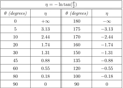
1.1 Classification and properties of leptons. . . 4 1.2 Classification and properties of quarks. . . 4 1.3 Classification and properties of the fundamental forces. . . 5 2.1 Some representative values of η and the corresponding polar

angle. . . 29 2.2 General performance goals of the ATLAS detector. . . 30 3.1 Jet trigger menu foreseen for the beginning of data taking at

the LHC with a luminosity of 1031_cm−2_s−1_{. . . 59}

4.1 Information from cosmic muon run 90272. . . 64 4.2 Approximate position of the peaks seen in the η and φ

distri-butions of jets from cosmic muon run 90272. . . 70 4.3 Approximate coordinates of the noisy cells seen in the (η, φ)

maps of jets from cosmic muon run 90272. . . 72 4.4 Change in number of trigger and offline jets from cosmic muon

run 90272 after noisy cell removal. . . 73 5.1 Information concerning the data samples containing dijet events

generated with PYTHIA. . . 95 5.2 Approximate accuracy of intercalibration in η determined

from applying the method to truth jets from QCD dijet events generated by PYTHIA. . . 104 5.3 Approximate asymmetry of LVL2 jets from QCD dijet events

generated by PYTHIA before and after applying the correc-tions derived with intercalibration in η. . . 108

(28)

5.4 Approximate precision of the LVL2 jet energy scale from QCD dijet events generated by PYTHIA before and after applying the corrections derived with intercalibration in η. . . 114 5.5 Efficiencies and associated uncertainties of the cuts applied

to LVL2 jets from QCD dijet events generated by PYTHIA when using the intercalibration in η method. . . 115

(29)

A new accelerator at CERN, the LHC, will collide beams of protons with unprecedented conditions of energy and luminosity, extending the frontiers of high-energy physics. ATLAS is a general-purpose detector designed to cover the widest range of physics possible at the LHC. The LHC will deliver collision data at a rate of 40MHz. Thus, one fundamental system in ATLAS is the trigger, that reduces the data flow to a manageable storage rate of 200Hz.

At the LHC jets will be the most commonly produced objects. Properly identifying, calibrating and reconstructing hadronic jets in an event is a fundamental task of the ATLAS jet trigger. This, however, represents a great challenge for ATLAS, particularly because jets may constitute signatures or background, depending on the physics process.

The need for an extremely efficient jet trigger in ATLAS motivated the work presented in this thesis, which is divided in two parts. The goal is simple: to assess and develop methods to improve the performance of the ATLAS jet trigger. Because the LHC is not yet producing pp collisions, cosmic muon data and MonteCarlo simulations were used for the analysis.

First, cosmic muon runs were used to evaluate the performance of the three levels of the ATLAS trigger system in reconstructing the energy and position of the jets. The evaluation was done by comparison between the trigger reconstruction and the offline reconstruction.

In the second study a in-situ calibration method, called intercalibration in η, was applied to MonteCarlo simulated data. The plan was to try to determine if the method could be used with real collision data to validate and tune the calibration applied to trigger jets at Level-2. In particular, the ability for that calibration to produce a jet energy scale uniform in η was

(30)

evaluated.

The outline of this thesis is as follows. In Chapter 1, the Physics’ aspects relevant to the work, mostly related to the subject of jets, are briefly pre-sented. A more technical description of the ATLAS Experiment is presented in Chapter 2. Chapter 3 is devoted to explaining how jets are handled in ATLAS. Finally, Chapters 4 and 5 describe the studies done and the results obtained on the performance of the ATLAS jet trigger.

(31)

Physics Motivation

1.1 Introduction to the Standard Model of

Parti-cle Physics

Particle physics deals with the study of the most fundamental constituents of matter and the nature of the interactions between them. However, which particles are regarded as fundamental has changed (and continues to change) with time, as physicists’ knowledge increases. The current view, described by a theory referred to as the Standard Model (SM), is, nonetheless, very simplistic and encompasses two basic ideas. First, all matter is composed of fermions, i.e., 1

2-spin particles1. Second, these fermions interact with each

other by exchanging bosons, which are integral-spin particles1 _[1].

Addressing the fermionic sector first, particles can be divided into two families according to their physical properties: leptons (l), which have inte-gral electric charges, and quarks (q), which carry fractional electric charges [2].

The most familiar example of a lepton is the electron e−_{, but, in reality,}

six more leptons exist. They can be classified according to their physical properties (namely the electric charge Q and mass m) and quantum numbers - electron number (Le), muon number (Lµ) and tau number (Lτ) - and

fall naturally into three generations. This information is summarized in table 1.1. Actually, six more leptons exist, since each particle in table 1.1 has

1_{All particles in the Standard Model are assumed to be elementary, meaning they are}

(32)

an antiparticle pair. Thus, a similar table could be built for the antileptons, the only difference being that all the signs would be reversed. The positron e+ for example, carries an electric charge of +1 and has Le = −1. So, in

summary, a total of 12 different leptons exist [3]. Leptons

Generation Flavor Mass Q Le Lµ Lτ

First Electron, e 0.511MeV -1 1 0 0

Electron Neutrino, νe < 2eV 0 1 0 0

Second Muon, µ 105.658MeV -1 0 1 0

Muon Neutrino, νµ < 2eV 0 0 1 0

Third Tau, τ 1776.84MeV -1 0 0 1

Tau Neutrino, ντ < 2eV 0 1 0 1

Table 1.1: Classification and properties of leptons [4].

As for the quarks, they can be organized similar to the leptons. In par-ticular, six different flavors of quarks exist, they can be distinguished by their physical properties and quantum numbers and fall into three genera-tions as well. For quarks, the quantum numbers are strangeness (S), charm (C), beauty (B), and truth (T ). Table 1.2 summarizes the main properties of the quarks. Again, all signs in this table could be reversed to create a table for the antiquarks. Moreover, and this is a property that does not exist in leptons, each quark can carry one of three color charges - red, green and blue. The result is that a total of 36 different quarks exist [3].

Quarks

Generation Flavor Mass Q C S T B

First Up, u 1.5 − 3.3MeV 2/3 0 0 0 0

Down, d 3.5 − 6.0MeV −1/3 0 0 0 0

Second Charm, c ≈ 1.27GeV 2/3 1 0 0 0

Strange, s ≈ 104MeV −1/3 0 -1 0 0

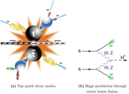
Third Top, t ≈ 171.2GeV 2/3 0 0 1 0

Bottom, b ≈ 4.20GeV −1/3 0 0 0 -1

(33)

Let us move now into the bosonic sector, which includes the elementary particles referred to as force mediators. The basic idea is that only four forces exist in nature strong, electromagnetic, weak and gravitational -and each one is described by a different theory. These are the forces by which the fermions interact with each other and they do so by exchanging a force mediator. In other words, the mediators carry/transmit the force from one interacting fermion to the other. Basically, mediators do so by coupling with the charges of the interacting fermions with a given coupling constant. Thus, the strength of a given interaction is determined by the value of its coupling constant. Table 1.3 summarizes the most relevant features of the Standard Model bosons. These will be developed next. [3]

Fundamental Forces Interactions Strong

Electro-magnetic Weak Gravitational

Charge Color Electric

Charge

Weak

Charge Mass

Relative

Coupling 10 10−2 10−13 10−42

Mediators 8 Gluons, g Photon, γ W−, W+

and Z Graviton

Fermion

Couplings quarks

all except

neutrinos all all

Table 1.3: Classification and properties of the fundamental forces [4].

The strong interaction, described by the theory of Quantum Chromo-dynamics (QCD) is, as suggested by the name, the strongest of the four interactions. It is mediated by the gluon (g), a spin-0, massless, neutral, elementary particle. At this point, it is important to say that gluons, as quarks, carry a color charge, which results in eight different gluons existing in nature. The color charge is, actually, the charge of the strong force, in the sense that only colored particles can interact strongly. Thus, the strong interaction is exclusive to quarks and gluons.

Quantum Electrodynamics (QED) is the oldest, simplest and most suc-cessful of the four theories and describes the electromagnetic interaction.

(34)

The electromagnetic mediator is the photon (γ), which, similarly to the gluon, has 0 spin, no mass and no electric charge. The photon can only cou-ple to electrically charged particles, which means that neutrinos are excluded from these interactions [3].

Weak interactions are described by Flavordynamics. The weak coupling constant is smaller than the strong coupling constant and the fine-structure constant (electromagnetic coupling constant), making the weak force weaker than the strong and electromagnetic forces. All quarks and leptons carry the ”weak charge”2_{, which means that all of them can couple to the force}

mediators and interact weakly. There are three different weak mediators: W+_{, W}− _{and Z. These bosons have spin-1, each one carries a different}

electric charge and, unlike the previous bosons, are very massive particles [3].

Gravity is the weakest of all four interactions. Classically it is described by Newton’s law of universal gravitation and its relativistic generalization is Einstein’s theory of relativity. However, a completely satisfactory quantum theory of gravity has not yet been worked out. Gravitons (gravity mediators) are hypothesized but, in reality, gravity is neglected in the field of elementary particles simply because it is too weak to play a significant role [3].

This short description of the SM would not be complete without men-tioning the Higgs boson, a massive particle with no intrinsic spin. Basically this boson is necessary in the SM to account for the masses of all elementary particles. In other words, without the Higgs, all particles would be mass-less, which experiment has shown not to be true. It is the coupling between the Higgs boson and the particles (including the Higgs itself) that generates their masses [1].

Currently, the Standard Model is in full agreement with the available experimental data accumulated over the past three decades. Actually, the SM provides some of the best agreements between theory and experiment in physics3_{. Nonetheless, physicists know it is not a complete theory. For}

example, the masses of SM particles are empirical numbers taken from ex-periment. This and other examples add up and the result is the SM has

2_{Quotation marks are used because no particular name exists for this charge}

3_{SM predicted the anomalous magnetic moment of the electron in agreement with the}

(35)

over 20 arbitrary parameters. Then, there is the opposite situation, where theoretical predictions have not yet been experimentally observed, such as the existence of the Higgs boson. Consequently, and despite its success, the interest in possible extensions or alternatives to the Standard Model continues to grow [5].

1.2 Jet Physics

1.2.1 Jet Phenomenology

As mentioned in the previous section, Quantum Chromodynamics (QCD) is the theory that describes the strong interactions that occur between color-charged particles. These can be quarks (q) or gluons (g) and they will be referred to as partons [6].

It is hypothesized in QCD that every naturally occurring particle should be a color singlet. This is called color confinement and it has several con-sequences. For example, it explains why isolated quarks have never been observed and why they only exist in bound states forming colorless systems - the hadrons. Also, it is the reason why only two types of hadrons are known. To produce a composite particle with no color, quarks can only be confined in two ways. Thus, there are only mesons - a quark and anti-quark bound state - and the baryons, formed by three quarks or three anti-quarks [7].

Although never derived from the theoretical QCD background, the ex-perimental observations mentioned in the previous paragraph support the idea of color confinement. Furthermore, some theoretical considerations in-dicate that the hypothesis is valid. In particular, the energy (or distance) dependence of the strong coupling constant, αs (figure 1.1).

The increase of αs for low energies, or equivalently the increase of the

strong interaction strength for long distances, strongly suggests the idea of quarks being clumped together, since trying to separate them would greatly increase the energy of the system [7].

Another important feature of αsis that it decreases at very high energies,

which is why the strong interaction strength vanishes at very short distances. Thus, as two quarks come closer and closer together, the strong force binding them weakens. This is called asymptotic freedom and it also suggests that

(36)

Figure 1.1: Energy dependence of the strong coupling constant αs (combined

results from several experiments) [8].

bound states of quarks are more stable than separated quarks, since they are almost ”free” [7].

One way to explain asymptotic freedom in QCD is to compare color-charge to QED color-charge. Take, for example, an electron. Its observed color-charge becomes smaller at larger distances or, in other words, the electric field weakens with the increasing distance. This is because of the screening of the electric charge by vacuum polarization, which is depicted in figure 1.2. What happens in QED is that the vacuum constantly sprouts particle-antiparticle pairs, such as electron-positron pairs, behaving like a dielectric medium. As the electron is placed in this dielectric vacuum, the positrons of the pairs will be attracted, while the electrons will be repelled, causing the vacuum to polarize. The average effect of this behavior is to partially cancel the field created by the electron. Thus, as one moves closer and closer to the electron, the screening effect starts disappearing, increasing the effective charge of the electron [3].

Comparatively to QED screening, the color of a quark is also shielded by the creation of quark-antiquark pairs in the vacuum. Nevertheless, there

(37)

Figure 1.2: Screening of the electric charge in QED [9].

is a fundamental difference between QED and QCD. The mediators of an electric interaction, the photons, have no electric charge, whereas the medi-ators of the strong interaction, the gluons, carry themselves a color charge. This means, for example, that gluons can couple between them and photons cannot. In fact, the emission of virtual gluons in the vacuum suppresses the emission of quark-antiquark pairs. Also, because gluons actually carry two color charges, they end up not screening the color field but rather increasing it. This is often referred to as antiscreening and is portrayed in figure 1.3. QCD antiscreening dissipates as one moves closer to the quarks, just as the screening effect for an electric charge. However, in QCD, the effective charge of the quark decreases. In summary, as the distance is increased, the strong interaction is strengthened, whereas for short distances the strong interaction field is very weak and quarks are nearly ”free” particles [3].

(38)

Figure 1.3: Screening of the color charge in QCD [9].

important consequence: the existence of jets. Suppose one has a baryon, such as the proton depicted in figure 1.4, and tries to separate one of the quarks from the other two. Due to asymptotic freedom the quarks are essentially free within the baryon. As one tries the separate them, i.e., in-crease the distance between the quarks, the interaction between them grows stronger, since color confinement does not allow the quarks to exist isolated. As the strong force tries to approximate the quarks back, it becomes, at some point, energetically more favorable to create a quark-antiquark pair from the vacuum than to separate the quarks from the baryon any further [9].

In summary, trying to break-up the hadron resulted in two new hadrons being created with no free quarks being obtained, as shown in figure 1.4. Thus, trying to observe isolated quarks (or gluons) results in several

(39)

quark-Figure 1.4: Possible scenario of color confinement of quarks. [3]

antiquark pairs being created. These join together in a myriad combina-tions resulting in the production of jets, through a process referred to as hadronization [3].

Basically, a jet is a collimated stream of colorless particles: mesons, baryons, leptons, photons. It emerges along the expected flight path of the primordial quark or gluon (since gluons carry color themselves they hadronize into jets just like quarks). Jets are, thus, the materialization or signatures of quarks and gluons [10].

The biggest challenge when it comes to jets is that hadronization is a non-perturbative process, since αs increases for long distances. This means

that it is not simple to understand jets on a theoretical point of view, since calculations are usually impossible. For example, one cannot calcu-late the content of photons in a particular jet. In fact, hadronization is explained mostly through models obtained from approximate treatments to QCD. Nonetheless, methods have been developed that allow the association of the visible jet to the non-visible quark or gluon that originated it. This will be developed in the following sections [8, 11].

1.2.2 Jet Production

As mentioned in the previous chapter, trying to obtain isolated partons originates jets. Jets were observed for the first time in the late 70’s by the JADE experiment at PETRA. At PETRA, electron-positron collisions took place. Some of those collisions originated a quark-antiquark pair: e+₊

e−_{→ q + ¯q. The pair eventually hadronized and the resulting particles were} observed as two back-to-back jets by the JADE detector. Sometimes,

(40)

three-jet events were observed as well. The third three-jet was interpreted as the result of the hadronization of a gluon radiated by one of the produced quarks. Thus, the three jet configuration was regarded as the most direct evidence of the existence of gluons and of their hadronization into jets [10, 3].

Figure 1.5: Cross sections for several processes as a function of √s from pp collisions [12].

Jets are also commonly produced in hadron-hadron colliders. This is understandable, since this type of colliders aims at breaking-up the hadrons, and is shown in figure 1.5. It presents the cross sections (σ) for several processes, occuring through proton-proton (pp) collisions, as a function of the center of mass energy (√s) and at a luminosity (L) of 1034_cm−2_s−1

[12]. Roughly, σ gives the probability at which a certain process occurs. This means that the higher the cross section of a certain process, the more likely it is that this process will come as a result of the collision. Thus, the rate (dN

(41)

particular, one has dN

dt = σ × L. Basically, L is the luminosity and measures

the density of particles in the colliding beams. It can be integrated over time, to obtain the integrated luminosity - L =! Ldt - in which case, the number of events is given by N = σ × L [13].

Taking this into account and analyzing figure 1.5, one can see that for pp collisions and hadron-hadron collisions in general, jet production is by far the process with the largest cross section, meaning that jet events are, indeed, very common in hadron colliders. This evaluation can be done on a more quantitative level, by considering the LHC, a hadron collider whose working conditions are indicated by the dotted line in figure 1.5. The total cross section for pp colisions at the LHC is σLHC

total ≈ 100mb [14]; for dijet

production at the LHC one has σLHC

dijet ≈ 0.4mb [15]; and the production of

a 100GeV Higgs boson through gluon fusion has a cross section of σLHC Higgs ≈

44pb [16].

It is clear now that understanding hadronic collisions is necessary to do studies on jets. Those studies can go from building MonteCarlo programs that simulate jet production, allowing some predictions to be made, to in-terpreting experimental results on particle detectors. To analyze the main aspects involving hadronic interactions and the production of jets, let us consider an event where two jets are produced. The production process is defined by p + p → jet + jet + X, where p are the colliding protons and X represents everything else produced in the collision. A schematic diagram of this scattering process is displayed in figure 1.6 [17].

(42)

The scattering process in figure 1.6 can be divided into the hard scat-tering part and the soft scatscat-tering part. QCD is the underlying theory that describes both parts. It is, however, more easily applied to the hard scatter-ing part of the process than to the soft part, where non-perturbative effects dominate. Thus, separating the full scattering process into several distinct steps is essential to understand it. These steps are presented in detail next [17].

The first step is the hard collision of two incoming partons, which can be represented by the diagram in figure 1.7. The two partons, one in each colliding hadron, are scattered at wide angles after passing very close to each other and, as a result, outgoing partons are produced. This is actually the process of particular interest, since the outgoing partons will eventually hadronize and be observed as jets of particles. This subject will be further developed in the section 1.2.3.

Figure 1.7: Feynman diagram for the scattering of two quarks [3].

The relative probability of finding the scattering partons at this step is provided by the parton distribution functions (pdfs). Roughly, the pdf of a certain parton reveals ”how much” of that parton exists in the colliding hadron at a certain energy scale, defining the parton uniquely [17].

The other elements visible in figure 1.6 (X), besides the partons/jets produced by hard scattering, are the result of several soft processes, which will be described next.

The two partons that undergo hard scattering can, before scattering, emit radiation, producing showers that constitute the initial state radiation

(43)

(ISR). The same process can occur with the outgoing partons from the hard scattering, before they hadronize, creating final state radiation (FSR) [13].

As for the partons remaining from the original hadrons, i.e. the ones that did not suffer hard scattering, they will interact softly with each other, scattering at small angles and generating the underlying event (UE). The UE, together with the ISR, produce the so-called beam remnants, which can suffer soft multiple interactions between them as well.

Finally, it is also important to mention minimum bias events. In a scat-tering process between two hadrons, often the hard scatscat-tering part does not occur, which means that all partons interact softly. Thus, in a high-luminosity regime, where the number of interacting hadrons per unit of time is high, if a scattering process between two hadrons occurs with the hard part, it will be accompanied by additional and uncorrelated soft processes from the interaction of the other hadrons. The products from these addi-tional soft interactions will pile-up with the products from main scattering processes [13].

1.2.3 Jet Reconstruction

In the previous section, the subject of jet production in hadron-colliders was addressed. In summary, when two protons collide, the process of interest is the hard scattering between two partons, that produces high momentum outgoing partons. These partons eventually hadronize into jets of particles. Those jets are observed in particle detectors as multi-particle signals. This is depicted in figure 1.8, if one reads it in the upward direction, following the ”jet production” arrow.

The goal at this point is to interpret the observed jet signals in terms of the underlying partons, i.e., to reconstruct the jets. Jet reconstruction is, thus, equivalent to reading figure 1.8 in the downward direction. The basic idea behind it is that one should be able to perform jet reconstruction on different objects - partons resulting from the hard scattering (”parton jet”), particles resulting from the hadronization of those partons (”particle jet”) and detector signals resulting from those particles (”calorimeter4 _{jet”) - and}

4_{The expression ”calorimeter jet” is employed because calorimeter signals are the most}

commonly used signals for jet reconstruction; nonetheless, other detector signals can be used, such as tracks.

(44)

Figure 1.8: Representation of the stages of jet production / jet reconstruction.

obtain the same jet without ambiguities or biases [18, 17]. The main aspects concerning jet reconstruction are described in the following sections. 1.2.3.1 Jet Identification

The first step in jet reconstruction is to identify the jet by means of a jet algorithm. A jet algorithm is, basically, a set of rules that defines the jet [18].

First, the algorithm identifies and clusters the objects that belong to the jet, whether those objects are real and obtained experimentally or generated and simulated with MonteCarlo. They can be detector signals, particles re-sulting from the hadronization or partons rere-sulting from the hard scattering. Then, the jet algorithm provides a recombination scheme that determines the properties of the jet as a function of the properties of the objects that make it. Usually it is a four-momentum (E, −→p ). The jet algorithm works in such a way that the properties of the jets can be, ultimately, related to the properties of the partons resulting from the hard scattering. In other words, a jet algorithm allows us to see the fingerprints of the partons in the

(45)

observed final states [19].

An ideal jet algorithm should possess certain attributes, both theoret-ical and experimental. As elucidated in figure 1.8, where the dotted cone represents the jet algorithm, the attributes are meant to minimize the differ-ence between reconstructed ”calorimeter jets”, ”particle jets” and ”parton jets”. In other words, and taking into account what was said in the previous section, the attributes of an ideal jet algorithm ensure that the same jet is always identified, regardless of which object the algorithm is applied to [19].

Figure 1.9: Representation of infrared sensitivity of a jet algorithm [19].

On the theoretical point of view, a jet algorithm should have the following attributes [19]:

• Infrared safety - This basically means that a jet algorithm should be insensitive to soft radiation. As shown in figure 1.9, if the algorithm is infrared safe, the two signals (represented by arrows in the right) would be reconstructed as two separate jets (represented by the cones). In an infrared sensitive algorithm, the two jets could be merged into one jet (cone on the right) due to the presence of soft radiation between them (wavy arrow).

• Collinear safety - If a particular signal is split into two equivalent and collinear signals, the reconstructed jet should remain unchanged. This is depicted in figure 1.10. Basically, if the algorithm is collinear safe, the jet (cone) would not change due to the splitting of the signal (long arrow on the left) into two (on the right).

• Invariance under boosts - This attribute ensures that the same solution is found independent of boosts in the longitudinal direction.

From the experimental standpoint, the attributes should minimize the effect of detector response, noise, pile-up, among others, on the jet identification process [19]:

(46)

Figure 1.10: Representation of collinear sensitivity of a jet algorithm [19].

• Detector independence - The algorithm should perform independent from the detectors characteristics, such as noise, response, segmenta-tion or resolusegmenta-tion.

• Stability - The jet algorithm should show stability with luminosity, meaning that the size of the jet should not be affected if other parton hard scatterings occur at high luminosities.

• Efficency - A jet algorithm should be efficient and easy to implement, identifying all physically interesting jets with minimum computing time.

• Ease of calibration - A jet algorithm should present no obstacles to the calibration of the properties of the reconstructed jet; this subject will be developed in the following section.

• Fully specified - The jet identification process must be fully specified, which includes clear definition of all the procedures, namely clustering and determination of the kinematic variables.

Several jet algorithms exist and part of the challenge is determining which ones are optimal for each specific physics analysis. Historically, cone algo-rithms have been the choice for hadron-hadron colliders. These algoalgo-rithms select objects close to each other and group them to form a cone-shaped jet in the (η, φ)-space (a two-dimensional space used commonly in hadron-hadron detectors). Though simple, fast and of easy implementation, cone algorithms presents some well known problems, such as the fact that the reconstructed jets can overlap and share energy and that they are not in-frared safe. Thus, a second class of jet algorithms has been developed and

(47)

proved more well behaved: the kT algorithms. With these algorithms, the

combination of objects does not depend solely on the distance between them but also on their kinematic properties [19].

1.2.3.2 Jet Energy Measurement

As shown in figure 1.8 and mentioned in the previous section, jets have to be reconstructed from the signals their particles leave in the particle detectors. Ultimately, the goal of jet reconstruction is to determine the properties of the original parton. However, identifying the jet by running a jet algorithm on detector signals is not enough to achieve this goal and calibration of the jet energy is fundamental to properly reconstruct the jet. The need for calibration of the jet energy is explained next [20].

Although other detectors, such as tracking devices, can be used, calorime-ters are, usually, the most relevant systems for jet reconstruction, hence the expression ”calorimeter jet”. Calorimeters have the role of determining the energy of the particles, which means jets are usually reconstructed from en-ergy depositions left in the calorimeters’ cells. Thus, understanding the way particles interact with calorimeters is necessary to understand the need for a calibration step in the process of jet reconstruction [17].

The basic mechanism that allows calorimeters to determine the energy of the particles is shower formation. Almost every particle5 _{that crosses a}

calorimeter, or any detection device, starts interacting with the nuclei of the materials that constitute it. As a result, secondary particles are produced with less energy than the original particles. Those secondary particles will also interact with the dense matter that forms the calorimeters and generate other less energetic particles. The result is a cascade of particles that devel-ops and grows until the only particles remaining are low energy ones that are stopped by the calorimeter and fully absorbed [21]. So, in summary, the energy of a particle is deposited gradually in the calorimeters, throughout the shower development. The calorimeters collect the energy and respond with a signal proportional to the amount of energy deposited.

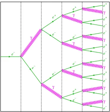
Showers can be classified in two types. Electromagnetic showers are usually initiated by photons or electrons/positrons and develop primarily

(48)

Figure 1.11: Simplified example of the development of an electromagnetic shower initiated by an electron.

through electromagnetic processes such as Bremsstrahlung or pair produc-tion (figure 1.11). Hadronic showers are, as the name indicates, initiated by hadrons, such as protons and neutrons. They develop mainly due to strong interactions between hadrons and the nuclei of the materials that compose the calorimeters [21].

The name ”hadronic” might actually be misleading because hadronic showers also have an electromagnetic component, since some hadrons are charged particles. For that reason, and also because hadrons, unlike elec-trons and photons, are not elementary particles, hadronic showers are usu-ally more complex and difficult to measure, treat, analyze or simulate than electromagnetic showers [22].

Figure 1.12 illustrates an important fact about hadronic showers, that is not observed in electromagnetic showers, called non-compensation. Es-sentially, calorimeters do not respond the same way to electromagnetic and

(49)

Figure 1.12: Example of the development of a hadronic shower [21].

hadronic showers6_{. The response of a calorimeter evaluates how much of the}

total energy of the particle is indeed collected by the calorimeter and one usually has e/h > 1, where e is the response of the calorimeter to the elec-tromagnetic component of a shower and h is the response to the hadronic component of a shower. Moreover, while e is approximately linear with the energy of the interacting particles, h is not. The reason for this has to do with the distinct way the two types of showers develop, as will be shown next [22].

To begin with, from the first time the primary hadron interacts with the nuclei of the medium that forms the calorimeter, a significant fraction of the energy is removed from further hadronic interaction. For example, particles such as the π0 marked in red in figure 1.12, decay into photons that then

generate high energy electromagnetic cascades. This fraction of the energy (≈ 50%), because it is of electromagnetic nature, is actually well determined by calorimeters [4, 22].

However, as charged secondary particles (such as π±_{, p, ...) interact}

with nuclei, they can either ionize (”non-EM energy” shown in black in the figure), or generate nuclei in excited states, fragments of nuclei and particles like muons and neutrinos. The energy to excite a nuclei or break it

6_{In reality, there are calorimeters that do not exhibit this behavior, but for the}

(50)

up generates little or no detectable signal and neutrinos and muons can cross calorimeters undetected. Consequently, these phenomena originate energy that is not collected by the calorimeters. In the end, a significant fraction of the hadronic energy - 20% − 30% depending on the calorimeter and the energy of the incident particle - is ”invisible” or has ”escaped” (blue and green in figure 1.12) [4, 22].

Taking this into account and since jets are of hadronic nature, it is clear that non-compensation can greatly influence the reconstruction of calorime-ter jets. In fact, other detector effects such as noise, dead macalorime-terial and detector signal efficiencies, or even physics effects, like pile-up, underlying event and jet identification algorithm efficiencies, will affect the reconstruc-tion as well. Moreover, the goal of jet reconstrucreconstruc-tion is to obtain jets at parton level, since it is the originating parton that constitutes the reference. However, the energy of the parton is not influenced by the mentioned de-tector and physics effects. Thus, one expects the energy reconstructed for a calorimeter jet to be different (usually lower) than the real energy of that jet, i.e., the energy of that jet at parton level. Therefore, once calorimeter jets are identified, calibration of their energies is a fundamental step to their reconstruction [23].

The jet energy scale evaluates the difference between the energy of the reconstructed jets and the real energy of those jets. So in other words, the goal of calibration is to obtain a uniform and stable jet energy scale, as a function of the energy of the jets and the positions where they were identified in the detectors, minimizing the difference between the reconstructed and real energies [23].

Several calibration schemes exist but the basic concept behind the most commonly used consists of applying calibration weights to detector signals according to the type of signals, i.e., hadronic-like or electromagnetic-like [23]. This subject will be further discussed in another chapter.

(51)

The ATLAS Experiment

2.1 The Large Hadron Collider

Located in the French-Swiss border, the European Organization for Nuclear Research [24] (CERN) is a scientific research facility created in 1954. Having 20 European Member States, employing around 2500 people (physicists, engineers, technicians, designers) and receiving over 8000 visiting scientists, CERN is, nowadays, the world’s largest particle physics center.

To achieve its main goal of providing ”...for collaboration among Euro-pean States in nuclear research of a pure scientific and fundamental char-acter...”, CERN makes use of instruments like particle accelerators, which boost beams of particles to high energies before they are made to collide, and detectors, which are used to observe and record the results of these collisions. In particular, CERN holds the accelerator complex depicted in figure 2.1. It is a chain of machines, where particle beams are injected from one to the next and their energies are increased successively.

The latest addition to the complex is called the Large Hadron Collider [25, 26] (LHC). The LHC will accelerate and collide hadrons, protons and lead ions (which will not be addressed in this thesis), with unprecedented working conditions, that will change the world of particle physics. Not only it will allow the rediscovery of the Standard Model, permitting high precision tests of QCD, electroweak interactions and flavor physics, but also, hopefully, enable the search for new physics phenomena: Higgs boson, Supersymmetry (SUSY), dark energy and dark matter...

(52)

Figure 2.1: Schematics of the accelerator complex at CERN.

On September 10th_{2008 proton beams circulated successfully in the LHC}

for the first time. On September 19th_{, however, a helium leak caused damage}

to the accelerator and the operations were stopped for repair. At this point, it is scheduled that the LHC will be again ready for beam injection by mid-November 2009 [27].

The LHC [28, 26] is installed in the Large Electron-Positron (LEP, a previous collider at CERN) tunnel, 50-175 meters underground, spanning the boarder between Switzerland and France. It consists of two rings (beam pipes) with a circumference of 26660m, where the beams will circulate in opposite directions. To avoid collision between the beam and gas molecules, the beam pipes are kept at a ultrahigh vacuum reaching 10−13_{atm. The}

rings cross at four points - the interaction points - where the hadrons are made to collide and four detectors are placed. Figure 2.2 shows a diagram of the underground placement of the LHC and the four detectors at the interaction points.