Plans as structured networks of hierarchically and temporally related case pieces

Plans as structured networks of hierarchically and

temporally related case pieces

Luís Macedo (*), Francisco C. Pereira (**), Carlos Grilo (**), Amílcar Cardoso (**) (*) Instituto Superior de Engenharia de Coimbra, 3030 Coimbra, Portugal

([email protected])

(**) Dep. Eng. Informática, Univ. Coimbra, Polo II, 3030 Coimbra, Portugal ([email protected], [email protected], [email protected])

Abstract. This paper describes a representation of plan cases as a structured

set of goals and actions. These goals and actions are the unit pieces that form a case. These case pieces are related each other by hierarchical and temporal links (explanations) forming a tree-like network. We give importance not just to explicit links, i.e., links between case pieces which are concretely known, but also to implicit ones, i.e., possibly unknown links between case pieces. Each case piece is explained by antecedent links and explains other case pieces by consequent links. The retrieval of a case piece is mainly guided by its links and by its surrounding case pieces. Our concept of case piece usefulness is briefly explained. We discuss the benefit of reusing and directly accessing small case pieces from multiple cases for improving the Case-Based Reasoning (CBR) systems’ capability and efficiency to solve problems. We explain the importance of stepwise refinement in plan cases and also the role that temporal representation can take in the meaningful and coherent construction of planning problem solutions.

An application in musical composition domain is presented. We also show how a musical composition task can be treated as a planning task.

1 Introduction

Considering cases as set of pieces (Barletta & Mark, 1988), also called snippets (Kolodner, 1988; Redmond, 1990; Sycara & Navinchandra, 1991) or footprints (Veloso, 1992; Bento, Macedo & Costa, 1994) instead of monolithic entities, can improve the results of a CBR system in that solutions of problems may result from the contribution of multiple cases.

Moreover, structured representations of cases (Plaza, 1995) allow treating pieces of cases as full-fledged cases, minimising the problems that appear when using parts of multiple monolithic cases, particularly, the lot of effort taken to find the useful parts in them.

Although many CBR systems select out cases that are most similar to the new problem, other selection criteria may prove more effective. E.g., Kolodner (Kolodner, 1989) has considered that the most useful cases are those that can address the reasoner’s current goal, which means that they may not be the most similar ones.

Knowledge-based retrieval systems (Koton, 1989) are a consequence of combining nearest neighbour and knowledge-guided techniques. These systems are characterised by the use of domain knowledge to the construction of explanations

for why a problem had a particular solution in the past. Explanations are necessary to similarity judgement (Barletta & Mark, 1989; Cain, Pazzani & Silverstein, 1991; Veloso, 1992; Bento & Costa, 1994). CBR is appropriate for domains where a strong theory does not exist but past experience is accessible. This leads to the consideration of cases imperfectly explained (Bento, Macedo & Costa, 1994).

A plan is a specific sequence of steps (or actions) with the aim of a goal achievement. Case-Based Planning (CBP) systems reuse past sequences of actions from past plans to construct new ones. Some systems like CELIA (Redmond, 1990), MEDIATOR (Simpson, 1985), JULIA (Kolodner, 1989; Hinrichs, 1988), PRODIGY/ANALOGY (Veloso, 1992), and CAPlan/CbC (Munõz-Avila & Huellen, 1995) break up the goal into smaller sub-goals, enabling plan construction by composition of sub-plans. This leads to an hierarchical representation of plan cases (Khemani & Prasad, 1995). The case representation is similar to a tree where each node is a goal and its sons the sub-goals, or at the latest level, the actions of the plan. Each goal (or action) depends on other goals. This is particularly evident in structured domains (Munõz-Avila & Huellen, 1995).

In this paper we will focus on a structured representation for plan cases as a set of implicitly and explicitly, hierarchically and temporally related case pieces. Each one of these case pieces is considered, for indexing, matching, retrieving and validation purposes, as an individual case, which facilitates the reuse of parts of multiple cases to construct a new solution.

To represent time, we adopt a kind of ‘‘pseudo-date’’ scheme (Allen, 1991; Grilo, Pereira, Macedo & Cardoso, 1996), which provides an efficient and expressive mean to represent and reason about time relations, even when dealing with incomplete information, as when incrementally constructing a solution from the adaptation of ill-related pieces. As we’ll exemplify in Section 5, this kind of representation also facilitates the retrieving process.

Our approach to case representation is presented in the next section. In section 3, we introduce the retrieval and plan generation processes. Section 4 presents an application in the music composition domain. We also explain how a music composition process may be seen as a planning task. A short example of new case generation is presented in section 5, and the handling of “pseudo-dates” is also exemplified. In section 6 we discuss some of the advantages of our approach. At last, a conclusion about our work is made in section 7.

2 Case Representation

2.1 Case Structure

Within our approach a case plan is a set of goals and actions organised in a hierarchical way (Figure 1): a main goal (the main problem) is refined into

sub-goals (the sub-problems), and so on, until reaching the actions (the leaf nodes of the tree1) that satisfy the goals.

Temporal Links g1 g22 g21 g 1 3 g2 g3 g g11 g12 g31 g32 α λ β ψ π Hierarchical Links a 1 1 2 a 1 1 3 a 1 1 1 a 1 1 4 a 2 1 1 a 2 1 2 . . . . . . . . . . .

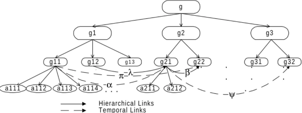
Fig. 1. Case structure. The g_i’s represent the goals and the a_i’s the actions.

In our model, each node of the hierarchical structure corresponds to a case piece. To complete the case structure, there are links between case pieces, representing causal justifications, or explanations. Some of these links maintain the hierarchical case structure, others reflect causal temporal relations between case pieces. Thus the existence of a case piece in a plan case is causally explained by several case pieces of the same plan case.

A measure of importance (strong, weak or medium) is given to each explicit link, according to its weight in the explanation of the consequent case piece.

Considering the hierarchical links only (represented in Figure 1 by continuous arrows), the inherent meaning of the represented structure is: g, the main goal of the plan (or the main problem), is achieved by sequentially achieving sub-goals (sub-problems) g1, g2 and g3. Each one of these sub-goals is also broken up into other sub-goals. For example, g1 is broken up into g11, g12 and g13, and g2 into g21 and g22. To achieve the goal g11 the actions a111, a112, a113 and a114 must be sequentially executed by this temporal order.

Besides being explained by the goal-refinement process, through hierarchical links, a case piece may also be explained through a temporal link (represented in Figure 1 by discontinuous arrows). For example, g21 (sub-goal of g2) is a consequence of case pieces g11 and g12, which is represented by the temporal links labelled α and

λ

As the case pieces form a tree-like structure we adopt the tree characteristic terminology to facilitate the description of our approach. Thus, we say that a case piece is a node and belongs to a level (e.g., in Figure 1, case pieces g1, g2 and g3 belong to level 1; case piece g belongs to the level 0). We also consider that father, son, brother, etc., relations exist between case pieces (e.g., in Figure 1, case piece g is father of case piece g1, g1 is son of g and brother of g2 and g3).

1_{Although the actions are represented by the leaf nodes, some of their properties}

We adopt Allen’s period-based approach to represent time2 (Allen, 1989), and associate a period to each case piece of the tree. A case piece’s position in the tree is represented by an address (“pseudo-date”) (see next section). Therefore, we may establish a correspondence between addresses and periods in a manner that simplifies the task of obtaining temporal relations (starts, meets, etc.) between case pieces, which is helpful for the temporal reasoning needed for plan generation, and also facilitates the use of causal temporal relations in the retrieval process.

2.2 Case Pieces

A case piece has seven types of information describing its relevant aspects: a name that uniquely identifies the case piece, the name of the case to which the case piece belongs, the case piece address, the constraints, a set of attribute/value pairs, the antecedents and the consequents.

The address of a case piece in level n is represented by Nn:Nn-1:...:N03, where

each

N

∈ℵ

<n, means that the case piece with that address has a predecessor in level i of the tree which is the L-th son of its father (with the exception of the case piece in level 0, which has no ascendants and so its offset is always 0). The offset J=Nn means that

this case piece is the J-th son of its closer ascendant. Every case piece propagates its address to its descendants, that is, if the case piece’s address is Nn:...:N0, its M-th

son’s address will be M:Nn:...:N0.

This representation embeds in its syntax, explicitly, the position that a case piece and its ascendants occupy in the tree relatively to the others, and, implicitly, the hierarchical level that the case piece occupies in the tree.

It is worth noting that the case pieces do not have all the same duration, and in consequence, each address is not committed with a fixed portion of time. We can say that a case piece has the length of its descendants, and that if it has not descendants, it has an intrinsic value (in the last level, the length of the actions that compose it).

Another information in a case piece is a set of attribute/value pairs describing several properties which characterise the case piece.

The constraints are also attribute/value pairs, but play the role of determining whether or not the case piece is a candidate to occupy a free position in a solution, depending on whether or not they are coherent with the attributes of the free position's hierarchical ascendants.

Antecedents and consequents are causal links that follow, respectively, from and to other case pieces. Antecedent links show how a case piece is explained by the existence of other case pieces (e.g. in Figure 1, g21 is explained by g11 and g12 through the links labelled

α

λ

2 _{We do not make any commitment about the discreteness or the continuity of time.} 3 _{Allen, uses ‘:’ to represent the “meets” relation. In our representation, ‘:’ is a}

(e.g., in Figure 1, g21 partially explains g22 and g32 through links

β

ψ

Each antecedent or consequent link is classified into another two main kinds of links: hierarchical and temporal ones.

Hierarchical links reflect the case pieces refinement (e.g., in Figure 1, there is a hierarchical link between goal g and goal g1 because g1 is a subdivision of g).

A temporal link expresses a causal explanation between two temporally disjoined case pieces (e.g., in Figure 1, case piece g21 is explained by case piece g11). The explanation embeds the causal temporal relation between the case pieces.

Sometimes the type of relation between antecedent fact(s) and the consequent one may be unknown. This lack of a complete theory is common in CBR (Bento, Macedo & Costa, 1994). This idea leads to another classification of the links between case pieces: we say that a link between the case pieces a and b is explicit if we known the relation between a and b, and implicit if we do not. In Figure 1, g13 implicitly (and temporally) explains g21. There is not a concrete link between them, but it is coherent to assume that the existence of g21 is, probably, partially due to the previous occurrence of g13. We may also say that a implicitly (and hierarchically) explains g21, although there is not a direct relation between them.

We call the case piece context to the set of case pieces that surrounds it. We distinguish eight types of contexts according to the kind of link existing between the case piece considered and the surrounding ones. Thus, each one of these surrounding case pieces is included in one of the following contexts (the name of the context reflects the classification of the link to the case piece): antecedent-hierarchical-implicit context, antecedent-hierarchical-explicit context, antecedent-temporal-implicit context, antecedent-temporal-explicit context, consequent-hierarchical-implicit context, consequent-hierarchical-explicit context, consequent-temporal-implicit context or consequent-temporal-explicit context.

For example, in Figure 1, the contexts of g21 are: hierarchical-implicit context = {g}; hierarchical-explicit context = {g2}; antecedent-temporal-implicit context = {g13}; antecedent-temporal-explicit context = {g11, g12}; implicit context = {}; consequent-hierarchical-explicit context = {a211, a212}; consequent-temporal-implicit context = {g31}; consequent-temporal-explicit context = {g22, g32}.

Since there is not any direct link between implicitly related case pieces, it is necessary to define a frontier to limit the number of case pieces of the implicit contexts. We assume that this frontier involves the nearest case pieces. To each implicit type of context, we defined a user-configurable parameter with the maximum distance a case piece may be to belong to a context of that type.

3 Retrieval and Plan Generation Processes

A new problem to be solved by the CBR system may comprise a set of linked case pieces. At least the main goal (the root case piece) must be included, with its name, address, constraints and attributes instanciated.

The meaning associated to a problem description composed by the main goal is the following: the system must find a structured plan solution to achieve the goal. If the problem also includes sub-goals or actions with the same instanciated information types, then the meaning of the problem description is augmented by the following: the system must find a structured plan solution to achieve the goal; the solution must achieve the specified sub-goals and perform the specified actions. Thus a problem may be a partial structured solution given by the user. The system just have to coherently complete it.

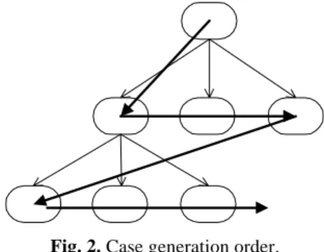
Fig. 2. Case generation order.

After giving the system a new problem, this is subdivided into several ones. Each one of these sub-problems is considered and solved individually, taking into account the previously solved ones.

Let’s give a sketch of the process. First, the main goal is considered. Since the complete information about this goal is not already known (for example, the number of sub-goals that are necessary to achieve it or the links that follow from it may be unknown), the main goal that best matches the considered one is retrieved from a case in memory. The next step is retrieving the main goal’s sons from memory, starting by the oldest, assuming its context (currently, the retrieved main goal), its attributes and its address as indexes. Following this, each one of these main goal’s sons is considered and its sons are retrieved from memory through a similar process. This procedure is repeated until the actions (the lowest level case pieces of the tree-like structure) are obtained. Figure 2 shows the sequence of the new case generation process.

The retrieving of a case piece from memory involves the following steps (given the context, the attributes and the address of the next free position on the new case4):

1) selection of the candidate case pieces from memory, eliminating those whose constraints are incompatible with the attributes of the free position’s ascendants, and those which do not belong to the same level of the free position;

4 _{The attributes of the free position may have already been instanciated by the user}

2) application of a similarity metric5 to each candidate case piece selected in step 1, taking into account the similarities between the given context, attributes and address and the context, attributes and address of the candidate case piece; 3) ranking of the case pieces by its similarity metric value;

4) selection of the most useful case piece;

5) validation of the addition to the solution of the selected case piece.

From the above algorithm it can be seen that the weighted similarity metric used for selection of a case piece takes into account the next three similarities

- attributes similarities, which are computed by the following way. Considering that α is the set of attributes of the considered free position on the new case, and β the set of attributes of the candidate case piece, then, the similarity between α and β is Y=[2*L(α∩β)]/ [L(α) + L(β)], where L(x) is a function that computes the length of the set x;

- address similarities, which are the result of two address similarity contributions: the absolute address similarity and the relative address similarity. The former one is 1 or 0, depending on whether or not the similarity between the two compared addresses is exact. The second one, takes into account the similarity of the temporal positions of the case pieces relatively to the beginning and to the end of the case. This temporal position is mapped into a interval between 0 and 1. Therefore, if a case piece is at the beginning of the case it has the relative temporal position 0, if it is in the middle 0.5, etc. These positions are then compared;

- context similarities. As was said above, we consider eight types of contexts. Each type of the free position's context is compared with the correspondent candidate case piece's context. Each type of context is an ordered set of case pieces, as we exemplified in section 2. The order is hierarchical or temporal, depending on the type of context. Therefore, the comparison between two correspondent contexts is performed taking into account not just their intersection, but also the similarity of the case piece’s order. This means, for example, that the contexts c1 = {a,b,c} and c2 = {b,c,a} (where a, b and c are case pieces), although their intersection is total, are not totally similar, because they have just one similar sequence of case pieces: c follows b.

In order to obtain meaningful case pieces associations, the similarity metric gives different weights to different context similarities. For example, it gives a bigger weight to explicit link’s similarities than to implicit ones.

The selection of the most useful case piece involves the computation of a similarity metric value for it and the consideration of the degree of matching the needs of the goal being achieved (Kolodner, 1989). Thus, the most useful case piece may not be the one with the most similarities. We think that this issue depends on the domain. Since our domain is music composition, an important parameter to consider is the originality of the new case, i.e, it is important that the new case has novel associations of case pieces, which are not present in the previous cases in memory. These novel associations may be required just in some hierarchical levels.

Therefore each one of the hierarchical levels has a selection criterion, which is defined by the user. This criterion determines which case piece is selected from the ranking. E.g., in level 1 the case piece selected is the totally similar, while in level 4 the case piece selected is the most but not totally similar.

After its selection, a case piece is submitted to a validation process consisting in the verification of incompatibilities between the selected case piece and the partially constructed solution for the given problem. At this point, there may be provisional links that follow from earlier case pieces, pointing to the free position. We call them suggestions, as they correspond to proposed but not definitive links. If an incompatibility exists between a suggestion and an antecedent link of the selected case piece there are two choices: (i) try to adapt it, relaxing the validation by ignoring the less important of the incompatible links (e.g., if the suggestion is strong and the antecedent link of the selected case piece is weak, the validation step substitutes the second link by the former one in the selected case piece, and then this case piece is added to the new case); (ii) if it was not possible to adapt it, select another one and apply the validation step to it.

4 An Application in Musical Composition Domain

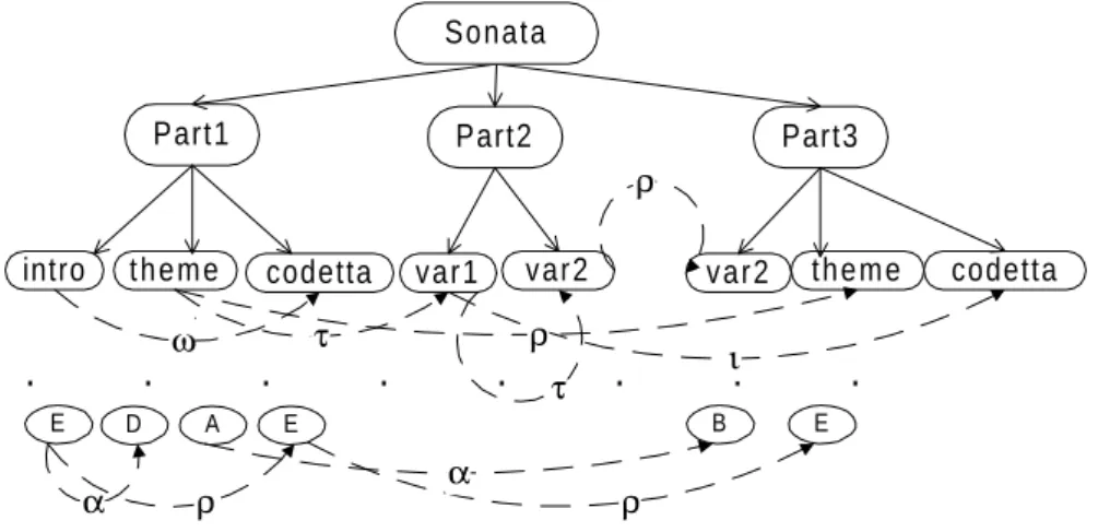
As studied by Lerdahl and Jackendoff (1983), Balaban (1992) and Honning (1993), music is a domain in which “structure”, “hierarchy” and “time” are more than occasional keywords. Music is indeed a highly structured and organised world. As stated by Balaban, any music can be represented by a hierarchy of temporal objects (an object associated with a temporal duration), in such a way that each one has, as descendants, a sequence of sub-objects that starts and ends at the same start and ending point as the object’s. Figure 3 shows an example.

.

.

.

.

.

.

.

.

intro t h e m e var2 codetta

ω τ τ ι t h e m e ρ ρ D A E B E E α ρ α ρ

Fig. 3. A case in the music domain.

In such a structure, we may say that each object has a temporal duration associated with it. We also may infer from that structure temporal relations between the objects. For instance, in Figure 3, we may infer (using Allen’s approach (1983)) that Part2 is during Sonata, met-by Part1, meets Part3, and is started by var1.

Apart from these temporal relations, there are also causal ones in music (represented in Figure 3 by discontinuous arrows), since many musical objects may be causally explained by, for instance, concretely known transformations of some other object (e.g., repetition, variation, inversion, transposition, etc.). For example, in Figure 3, the temporal link between theme of Part1 and var1 of Part2 may represent a variation transformation which, when applied to theme originates var1. These temporal relations are represented in the antecedents and consequents informations fields of a case piece.

Each musical object has several properties which are represented in our approach by attribute/value pairs (e.g., {ton='I', meas=2/4} meaning that tonality is 'I' and that measure is binary).

Additionally, each musical object has also a set of constraints, which are conditions that must not be contrary to the attributes of its ascendants, when it is added to the new case (e.g., if a case piece has the set of constraints a = {meas=2/4, ton='II', etc} then it must not be a descendant of a case piece which tonality is, for example, 'I'). Thus the role of constraints is to maintain the coherence of the new musical piece hierarchy, since they disallow the hierarchical association of case pieces with incompatible properties.

The goal of our application is to use analysis of music pieces as foundation for a generative process of composition, providing a structured and constrained way of composing novel pieces, although keeping the essential traits of the composer’s style. We use analysis of music pieces from a seventeenth century composer.

We have concluded that considering music as a plan, with the organisational characteristics described earlier, and the act of composing as CBP, might be an interesting way of generating new music from old ones. In fact, music structure has the basic conditions to be considered as a normal plan structure.

5 An Example

In this section we illustrate the new case generation in music domain.

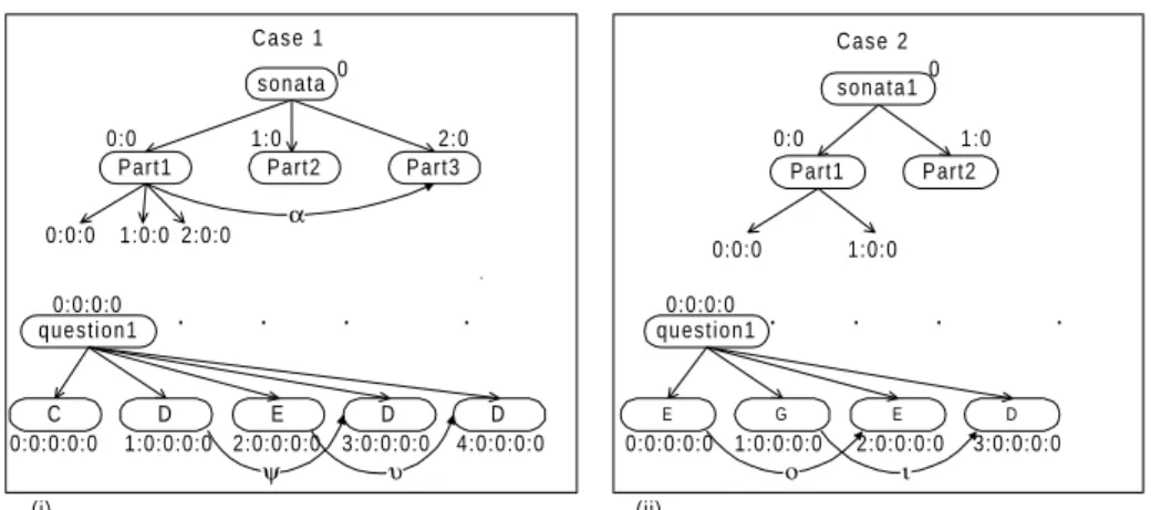
(i) question1 D C E D D ψ υ Case 2 question1 G E E D ο ι 0:0:0:0 0:0:0:0:0 sonata Part2 Part3 Part1 α Case 1 0:0 1:0 2:0 0:0:0 1:0:0 2:0:0 sonata1 Part2 Part1 0:0 1:0 0:0:0 1:0:0 0:0:0:0 0 0 1:0:0:0:0 2:0:0:0:0 3:0:0:0:0 4:0:0:0:0 0:0:0:0:0 1:0:0:0:0 2:0:0:0:0 3:0:0:0:0 . . . . (ii)

At the beginning, the system’s memory has two musical cases (represented in Figure 4)6.

The problem given to the system (represented by the PROLOG fact case_node(new_case, sonata2, 0, [], [ton='I',meas=2/4, style=sonata], [],[])) is to come up with a music sonata (style=sonata) characterised by having binary measure (meas=2/4) and tonality ‘I’' (ton=’I’).

First, a case piece with more similarities with the one represented in the problem is retrieved from a case in memory.

The system retrieved the main goal of case 1 since it is the one with more similarities with the main goal of the problem. At this point the solution is the one presented in Figure 4 - (i).

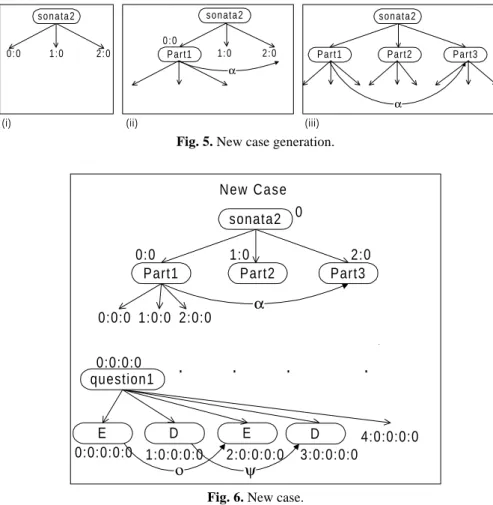
s o n a t a 2 Part2 Part3 Part1 α s o n a t a 2 Part1 α 0 : 0 1 : 0 2 : 0 0 : 0 1 : 0 2 : 0 s o n a t a 2

(i) (ii) (iii)

Fig. 5. New case generation.

question1 D E E ο 0:0:0:0 0:0:0:0:0 1:0:0:0:0 2:0:0:0:0 sonata2 Part2 Part3 Part1 α New Case 0:0 1:0 2:0 0:0:0 1:0:0 2:0:0 0 ψ D 3:0:0:0:0

.

.

.

.

Fig. 6. New case.

Next step is retrieving a case piece from memory to be placed on the new case free position with address 0:0.

This free position belongs to the first level of the tree. Therefore, the candidates are those ones belonging also to the first level of the two cases. There are five candidates: Part1, Part2 and Part3 from case 1, and Part1 and Part2 from case 2. Part2 from case 2 is eliminated since it has the constraint ton=’II’, which is incoherent with the attribute ton=’I’ of case piece Sonata2.

To apply the similarity metric, the system has to compute the context of the free position 0:0 and of all candidates. It takes use of the address to more easily perform this task. Thus, for example, the surrounding case pieces of Part2 (address 1:0 of case 1) are obtained as follows: the father is obtained deleting the first offset (1); the immediately younger brother is obtained subtracting 1 to the same first offset and maintaining the rest of the address, etc.

The system ranked the candidate case pieces by the following decreasing similarity order: Part1 (address 0:0 of case 1), Part1 (address 0:0 of case 2), Part2 (address 1:0 of case 1) and Part3 (address 2:0 of case 1). The selection of one of these pieces depends on the used criterion for this hierarchical level, which is to select the most similar case piece. Therefore Part1 (0:0 of case 1) is chosen. Since it has not incompatibilities with the other case pieces of the current solution, it is added to it (Figure 5 - (ii)). It can be seen that exist a suggestion between addresses 0:0 and 2:0.

Next step is the retrieval of a case piece for the new case free position with address 1:0, and then to 2:0. The system chose Part2 and Part3 from case 1, respectively (Figure 5 - (iii)). At this level, as a consequence of the selection criterion be to select the most similar case piece, there are no originality in the new case, since it is equal to case 1.

From Figure 6, which presents the final new case, it can be seen that the system selected the note E (address 0:0:0:0:0 of case 2) for position addressed with 0:0:0:0:0, since the selection criterion was to select the second most similar case piece in the ranking (the first is C from address 0:0:0:0:0 of case 1). To the address 1:0:0:0:0 it selected D (address 1:0:0:0:0 of case 1), since G (address 1:0:0:0:0 of case 2) is the most similar. And so on.

Consequently, at this level and using this criterion, the system obtained novel associations of case pieces. If the criterion was to select the less similar case piece, then more novel associations were made, and therefore, the new case was more original, but probably, it was also more bizarre.

6 Discussion

Our approach to case representation has some similarities with CELIA's (Redmond, 1990) which are mainly: cases are stored in pieces; there are links between case pieces to maintain the structure of the case; case pieces are accessed taking into account the case piece context; a case is constructed with case pieces of multiple cases.

However there also some key differences. The major ones are: rather than considering just hierarchical links we also assume the existence of temporal ones; rather than considering just explicit links we also assume the existence of implicit

ones; we use a representing time technique based on ‘’pseudo-dates’’ (the case pieces' addresses).

Our representational approach exhibits several advantages for CBP (some of them are common to CELIA's advantages).

Storing cases as individual pieces facilitates the access to all useful case pieces from several cases, improving the efficiency of retrieval. CBR systems dealing with monolithic cases have two steps to access the useful parts of previous cases: they need to retrieve the whole case and then they take a lot of effort to find its relevant part(s).

Moreover, the retrieval efficiency is increased by a simplified search of the case piece context, provided by using the addresses. In fact, the properties of the address and the links of the case piece together allow a fast collecting of the surrounding case pieces (case pieces of the context).

An issue worth of addressing is the case pieces size, because CBR systems’ efficiency and capability to solve new problems depend on that. It could be expected that a system dealing with smaller case pieces would be less efficient than one dealing with bigger ones (or with no case pieces at all), because of the greater number of retrieval operations that have to be performed. However, this drawback is overwhelmed by providing direct access to the case pieces in memory, avoiding unnecessary processing.

We also think that the capability of a CBR system to solve problems grows when the case piece size decreases: using smaller case pieces, we may dispose of a higher number of combinations to construct the solution. The usefulness of a case is also improved because it is considered in terms of case pieces and not in terms of the all case. This means that, for example, a case as a all may have little usefulness to construct the new case, but may have a highly useful case piece for a free position of that new case, and then, may contribute with a case piece to it. If considered as monolithic cases, because of it little usefulness, that case probably would not be considered to contribute for the generation of the new case.

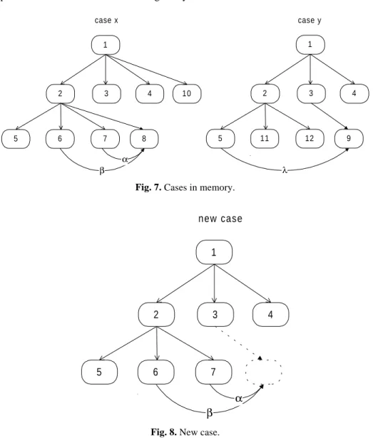
Some CBR systems do not consider temporal links between events. Figure 7 and 8 show the importance of these links to construct meaningful and coherent cases using case pieces assembling. Supposing we have two candidate pieces (8 and 9) to be put in the new case place represented by a discontinuous circle in Figure 8, retrieved, respectively, from case x and case y. Case piece 8 (case x in Figure 7) is temporally explained by case pieces 6 and 7, and hierarchically explained by case piece 2. Case piece 9 (case y in Figure 7) is temporally explained by case piece 5, and hierarchically by 3. The free position of the new case (Figure 8) is temporally suggested by 6 and 7, and hierarchically by 3. Thus, if we take into account just hierarchical links we select piece 9, but considering also temporal links then piece 8 is chosen (it is assumed that equal weights is given to all contexts in the similarity metric and that the address, and attributes contributions are not considered). So, piece 8 has a higher similarity value than 9. Thus, the system selected 8, and consequently, the case constructed is more coherent than if piece 9 was chosen. If we selected 9 instead of 8 the new case was more original, since we were making more novel case pieces associations (9 was original linked with two case pieces (6

and 7), while 8 is just original linked with one (3)), but is also with more probabilities a more bizarre one. This idea means that the selection order of case pieces determines the solution’s originality.

λ 1 3 4 2 11 12 5 9 β 1 3 4 2 6 7 5 8 α 10 case x case y

Fig. 7. Cases in memory.

β 1 3 4 2 6 7 5 α new case

Fig. 8. New case.

Our system can be used for solving problems in structured planning domains. In these domains, we distinguish two main kinds of problems: problems that do not require original solutions, i.e., if the same problem is proposed in different times it must have the same solution; and problems constrained to have original and useful solutions, i.e., the same problem has different solutions if proposed to the system in different times. The problem of finding an algorithm to a programming problem just need one solution (although it may have more). The problem of finding the less extent route between two sites in a city can have just one solution. Thus, these are

examples of the former kind of problems. In contrary, the problem of composing a sonata or writing a scientific fiction book, must not have previous solutions. These are examples of the second kind of problems.

To be applied for the first kind of problems, our system must have in every levels the criterion of selecting the most similar case piece, while to be applied for the second kind, the criterion must be, at least in one level, to not select the totally similar case piece. Thus, we may conclude that in these kind of problems the most useful case piece (Kolodner, 1989) is the one: (i) which gives more original case pieces associations to the new case; (ii) and that does not confront the coherence and meaningfulness of the new case.

7 Conclusions

We have presented an approach to representing structured plans as a combination of a tree-like network with a pseudo-dating scheme. Under this approach cases comprises a set of linked pieces.

Three main classifications of links were reported: implicit/explicit links; temporal/hierarchical links; and antecedent/consequent links.

These link classifications determine eight types of case piece contexts in which the retrieval process to new case generation is based.

As shown, musical composition can be considered as a planning task and is an appropriate domain to our approach. However, in this domain and other similar ones like story making or cook recipes generation, we think it is important to assume that a useful case piece (or case) may not be the one with the best similarity metric value but instead the one which gives coherently meaningful originality to the new case.

This approach is already implemented and is in test phase.

Acknowledgements

We would like to thank to Anabela Simões and António Andrade, teachers at the Coimbra School of Music for their valuable contribution, and the anonymous reviewers of this paper for their helpful comments.

References

Allen, J., (1983) - Maintaining Knowledge about Temporal Intervals. ACM 26(11), pp. 932-843.

Allen J., and Hayes, P., (1989) - Moments and Points in an interval-based temporal logic. Computational Intelligence, An International Journal, Vol. 5.

Allen J., and Hayes, P. J. (1991) - Time and Time Again: The Many Ways to Represent Time. International Journal of Intelligent Systems, Vol. 6, pp. 341- 355.

Balaban, M., (1992) - Musical Structures: Interleaving the Temporal and Hierarchical Aspects in Music. In Understanding Music with IA: Perspectives in Music Cognition, MIT Press, pp. 110 - 138.

Barletta, R., Mark, W., (1988). Breaking cases into pieces, in Proceedings of a Case-Based Reasoning Workshop, St. Paul, MN.

Barletta, R., Mark, W., (1989). Explanation-Based Indexing of Cases, in Proceedings of a Case-Based Reasoning Workshop.

Bento, C. and Costa, E., (1994). A Similarity Metric for Retrieval of Cases Imperfectly Explained. In Wess S.; Althoff, K.-D.; and Richter, M. M. (eds.), Topics in Case-Based Reasoning - Selected Papers from the First European Workshop on Case-Based Reasoning, Kaiserslautern, Springer Verlag.

Bento, C., Macedo, L. and Costa, E., (1994). RECIDE - Reasoning with Cases Imperfectly Described and Explained, in Second European Workshop on Case-Based Reasoning.. Cain, T., Pazzani, M. and Silverstein, G., (1991). Using Domain Knowledge to Influence

Similarity Judgements, in Proceedings of a Case-Based Reasoning Workshop, Morgan-Kaufmann.

Grilo, C., Pereira, F. C., Macedo, L. and Cardoso, A. (1996). A Structured Framework for Representing Time in Generative Composing System, International Conference on Knowledge Based Computer Systems’96. (submitted)

Hinrichs, T., (1988). Towards an Architecture for Open World Problem Solving, In Proceedings of a Workshop on Case-Based Reasoning, San Mateo, CA, Morgan Kaufmann.

Honning (1993). Issues in the representations of time and structure in music. Contemporary Music Review, 9, pp. 221-239.

Khemani, D., Prasad, P., (1995). A Memory-Based Hierarchical Planner, in Proceedings of the First International Conference on Case-Based Reasoning, Sesimbra, Portugal. Kolodner, J., (1988). Retrieving events from a Case Memory: a parallel implementation, in

Proceedings of a Case-Based Reasoning Workshop, San Mateo, CA, Morgan-Kaufmann. Kolodner, J., (1989). Judging Which is the “Best” Case for a Based Reasoner, in

Case-Based Reasoning: Proceedings of a Workshop, Florida, Morgan-Kaufmann.

Koton, P., (1989). Using Experience in Learning and Problem Solving, Massachusets Institute of Technology, Laboratory of Computer Science (Ph D diss., October 1988), MIT/LCS/TR-441.

Lerdahl, F. and Jackendoff, R. (1983). A Generative Theory of Tonal Music. Cambridge, Mass.: MIT Press.

Munõz-Avila, H., Huellen, J., (1995). Retrieving Cases in Structured Domains by Using Goal Dependencies, in Proceedings of the First International Conference on Case-Based Reasoning, Sesimbra, Portugal.

Plaza, E., (1995). Cases as terms: A feature term approach to the structured representation of cases, in Proceedings of the First International Conference on Case-Based Reasoning, Sesimbra, Portugal .

Redmond, M., (1990). Distributed Cases for Case-Based Reasoning; Facilitating Use of Multiple Cases, In Proceedings of AAAI.

Simpson, R., (1985). A Computer Model of Case-Based Reasoning in Problem Solving. PhD thesis, Georgia Institute of Technology, Atlanta, GA.

Sycara, K., Navinchandra, D., (1991). Influences: A Thematic Abstraction for Creative Use of Multiple Cases, in Proceedings of a Case-Based Reasoning Workshop.

Veloso, M., (1992). Learning by Analogical Reasoning in General Problem Solving, Ph D thesis, School of Computer Science, Carnegie Mellon University, Pittsburgh, PA.