OCEAN FORECASTS IN THE SOUTHWESTERN ATLANTIC: IMPACT OF DIFFERENT SOURCES OF SEA SURFACE HEIGHT IN DATA ASSIMILATION

(1)

“main” — 2014/1/16 — 15:48 — page 243 — #1

www.scielo.br/rbg

OCEAN FORECASTS IN THE SOUTHWESTERN ATLANTIC: IMPACT OF DIFFERENT

SOURCES OF SEA SURFACE HEIGHT IN DATA ASSIMILATION

Raquel Leite Mello

1

_{, Ana Cristina Neves de Freitas}

1

_{, Lucimara Russo}

1

_{, Jean Felix de Oliveira}

1

_,

Clemente Augusto Souza Tanajura

2

_{and Jo˜ao Bosco Rodrigues Alvarenga}

1

ABSTRACT.The objective in this paper is to analyze which Sea Surface Height (SSH) source applied to HYCOM (HYbrid Coordinate Ocean Model) is best suited to numerical prediction of the Southwest Atlantic Ocean. To this end two nested grids were used. One grid for the entire Atlantic Ocean (1/4◦_{) nesting the grid for the}

Southwest Atlantic (1/12◦_{) in the one-way mode. Three forecast experiments with different SSH data sources (Naval Research Laboratory – NRL; Archiving, Validation and}

Interpolation of Oceanographic Data – AVISO and MERCATOR) applied to constrain the initial conditions and a control forecast experiment without SSH constrain were compared. The comparison of forecasted temperature and salinity profiles with Argo data showed good correlation, over 0.98 for temperature and 0.87 for salinity. The NRL experiment – with SSH obtained by HYCOM+NCODA (Navy Coupled Ocean Data Assimilation System) GLOBAL 1/12◦_{analysis was the one that best represented}

the average temperature and salinity profile with respect to the Argo data.

Keywords: HYCOM, numerical modeling, ocean prediction, Argo profiler, Taylor diagram.

RESUMO.O objetivo deste trabalho é avaliar qual a fonte de dados de ASM (Altura da Superf´ıcie do Mar) imposta no modelo HYCOM (HYbrid Coordinate Ocean Model) é mais adequada para a previsão numérica do Oceano Atlântico Sudoeste. Para isto foram utilizadas duas grades aninhadas, uma grade para todo o Oceano Atlântico (1/4◦_{) aninhada no modo one-way a outra grade para o Atlântico Sudoeste (1/12}◦_{). Foram realizados três experimentos com diferentes campos de ASM (Naval}

Research Laboratory – NRL; Archiving, Validation and Interpolation of Oceanographic data – AVISO e MERCATOR) impostos na condição inicial e um experimento controle no qual não foi usada fonte de ASM externa. A comparação dos perfis de temperatura e salinidade entre os dados observados e os resultados do modelo apresentou boa correlação, maior que 0,98 para a temperatura e 0,87 para a salinidade. O experimento NRL com ASM total obtido dos resultados do HYCOM+NCODA (Navy Coupled Ocean Data Assimilation) GLOBAL 1/12◦_{foi o que melhor representou o perfil médio de temperatura e salinidade observado.}

Palavras-chave: HYCOM, modelagem numérica, previsão oceânica, perfiladores Argo, diagrama de Taylor.

1Centro de Hidrografia da Marinha (CHM), Diretoria de Hidrografia e Navegação (DHN), Rua Barão de Jaceguai s/n, Ponta da Armação, 24048-900 Niterói, RJ, Brasil. Phone: +55(21) 2189-3612 / 2189-3613 – E-mails: [email protected]; [email protected]; [email protected]; [email protected]; [email protected]

2Departamento de F´ısica da Terra e do Meio Ambiente, Instituto de F´ısica, UFBA, Campus de Ondina, Travessa Bar˜ao de Jeremoabo s/n, 40170-280 Salvador, BA, Brasil. Phone: +55(71) 3283-6685; Fax: +55(71) 3283-6681 – E-mail: [email protected]

(2)

INTRODUCTION

Oceanic and continental shelf regions are areas where large num-ber of activities have been developed, particularly the exploration of natural resources, either renewable or not, of great economic value. Tourism, shipping, leisure activities, fishing and oil explo-ration are just some examples. These areas are subject to serious environmental problems caused by accidents with vessels and operations associated with offshore oil exploration. Detailed knowledge of the dynamic of the waters, in their various temporal and spatial scales, is extremely important for studying environ-mental impacts, development plans and the execution of contin-gency plans in the event of accidents.

Due to the great demand for oceanographic information for application in the petroleum industry and for military activi-ties, a wide-ranging research network has been created, called “Oceanographic Modeling and Observation Network” – REMO (Portuguese acronym). The overall aim of REMO is the devel-opment of science and technology in physical oceanography, oceanic modeling, observational oceanography and operational oceanography with data assimilation.

At present, one of the challenges faced by the modeling branch of operational oceanography in Brazil is the implementa-tion of oceanic numerical models with data assimilaimplementa-tion. Over re-cent years, this has become one of the most efficient tools for char-acterization of the hydrodynamic of estuary, coastal and oceanic regions, so as to make the results of the models more accurate (Tanajura & Belyaev, 2002; Campos, 2006; Cirano et al., 2006; Chassignet et al., 2009; Dombrowsky et al., 2009; Fernandes et al., 2009; Kourafalou et al., 2009). Satellite measurements of sea surface height (SSH) are important for oceanographic studies, considering that in oceanic regions these measurements are very precise (Saraceno et al., 2010). Nevertheless, in coastal regions (distances less than 50 km from the coast), the data are normally of poor quality, as a result of various technical fac-tors, for instance: radar echoes in an onshore region, inaccuracy in corrections of the effects of tides and atmospheric pressure, among others (http://www.aviso.oceanobs/en/applications/coas-tal-applications.html). SSH represents part of the variations of the pressure gradient and, consequently, the barotropic circula-tion that takes place in the ocean. The effect of assimilacircula-tion of SSH on simulations of oceanic circulation can be investigated by the comparison of numerical experiments with and without assimila-tion, and observed data.

There are various methodologies for assimilation of observa-tional data into oceanic models: statistical correlations between

the altimetry data (SSH and/or SST) and variables that make up the mass fields of the oceans (T and S) are used to impose innova-tions on the vertical distribution of these variables (Mellor & Ezer, 1991; Ezer et al., 1993; Ezer & Mellor, 1994); methods of Opti-mal Interpollation that impose innovations on the fields predicted by the models, based on matrices of covariances of model errors (Oke et al., 2007, Counillon & Bertino, 2009; Oke et al., 2010); methods based on Kalman filters that use this technique to deter-mine the variability of the covariances of the model errors with a higher computing cost than optimal interpolation (Houtekamer & Mitchell, 1998), among others.

The objective of this work is to assess which source of SSH data is best suited to assimilation in the area of interest. Thus, three experiments were conducted with different sources of SSH. The results were compared with hydrographic profiles from Argo drifters. A control experiment was also performed in which no external source of SSH data was used.

METHODOLOGY

Description of the experiments

The hydrodynamic model HYCOM (Hybrid Coordinate Ocean Model) was used. This model employs hybrid coordinates and benefits from the advantages of the three coordinates traditionally used:

(i) isopycnal coordinates, which represent surfaces of con-stant density for modeling deep and stratified oceans; (ii) _{z levels that represent fixed levels of depth or of constant}

pressure, for modeling close to the ocean surface, that is to say, within the mixture layer, where higher vertical res-olution is required; and

(iii) sigma levels, used in regions with sharp topographical gradients, such as the transition between the Continental Shelf and the slope (Bleck, 2002; Halliwell, 2004; Chas-signet et al., 2003, 2006, 2007).

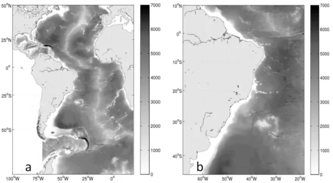
For the simulations, two grids were used, both with 21 verti-cal layers, a higher horizontal resolution grid nested in another grid of lower resolution. The grid with lower horizontal reso-lution, of approximately 28 km (1/4◦_{), takes almost the entire}

Atlantic Ocean with the domain from 50◦_{N to 78}◦_{S and from}

98◦_{W to 22}◦_{E (Fig. 1a). This grid has the Northern and}

South-ern edges closed and imposition of the transport of the Antarctic Circumpolar Current (110 Sv; 1 = 106_m3_{/s) and the Agulhas} Current (10 Sv) on the Eastern and Western edges, respectively.

(3)

“main” — 2014/1/16 — 15:48 — page 245 — #3

MELLO RL, FREITAS ACN, RUSSO L, OLIVEIRA JF, TANAJURA CAS & ALVARENGA JBR

245

Figure 1 – Bathymetry used in the HYCOM model for: 1a) grid with resolution of 1/4 degree for the entire Atlantic and 1b) grid with

resolution of 1/12◦_{for the Southwestern Atlantic. The gray scale indicates the depth in meters of each grid.}

This grid provides the boundary conditions in one-way mode for the grid with horizontal resolution of approximately 9 km (1/12◦₎

with the domain from 10◦_{N to 45}◦_{S and from 68}◦_{W to 18}◦_W

(Fig. 1b). This higher-resolution grid covers the Metarea V, which is an area of the Atlantic Ocean to the West of 20◦_{W between 7}◦_N

and 35◦₅0_{S over where the Brazilian Navy produces operational}

weather forecasts within the framework of the World Meteorolog-ical Organization (WMO) Marine Broadcast System for the Global Maritime Distress and Safety System.

The bathymetry used in the numerical experiments (Fig. 1) is derived from ETOPO21_{merged with detailed bathymetry from the}

Brazilian Directorate of Hydrography and Navigation (DHN) nau-tical charts database.

The atmospheric forcing used for the model integration were air temperature at 2 m, precipitation, total radiation, short-wave radiation, water vapor mixed ratio, and wind speed at 10 me-ters taken from the operational forecasts produced by the Global Forecast System (GFS) of the National Centers for Environ-mental Prediction/National Oceanic and Atmospheric Adminis-tration (NCEP/NOAA) (ftp://ftpprd.ncep.noaa.gov/pub/data/nccf/ com/gfs/prod/), with resolution of 1◦_{× 1}◦_{every six hours.}

This article discusses the results of a sequence of short-term ocean forecasting experiments during two months. The goal is to investigate the model sensitivity to different SSH data employed to construct the forecast initial conditions. The months of February and March were chosen for this work due to the quantity of

ob-served data available for comparison with the model results. For both grids, the model was initialized on February 2nd_{2010, based} on results of analysis of HYCOM+NCODA (Navy Coupled Ocean Data Assimilation) GLOBAL 1/12◦ _{obtained at the NRL (Naval}

Research Laboratory).

This work chose as an assimilation technique the Cooper & Haines (1996) scheme, which uses SSH data to calculate the new structure of the mass field of the water colunm, based on the conservation of mass. To achieve this, taking as a reference the innovations of the SSH fields, thicknesses of the adjacent layers below the mixed layer are modified, accompanied by the necessary modifications in the deep layers, so as to ensure that the height of the column is adjusted to the SSH innovation and conservation of mass maintained. The Cooper & Haines (1996) scheme has a low computing cost and is widely used in models where the SSH is not a prognostic variable, but is directly linked to the thickness of the isopycnals that represent the vertical co-ordinate and which together with the T and S variables define its mass field.

Data assimilation was performed at regions with depths greater than 200 meters for purposes of maintaining a standard for comparison, even in the experiments that assimilate data from other models, where data is available for shallower regions.

Three experiments were conducted with the grid of 1/12◦_to

insert SSH fields from different sources at the start of each fore-cast. The experiments performed were

1_{ETOPO2 Global Gridded 2-minute Database, National Geophysical Datacenter; National Oceanic and Atmospheric Administration, U.S. Department of Commerce,}

(4)

1) NRL – total SSH obtained from the results of HY-COM+NCODA GLOBAL 1/12◦_{obtained at the NRL;}

2) ALONG TRACK – SSH produced using the optimal inter-polation method with the along-track data in a seven-day window, furnished by the AVISO system (Archiving, Vali-dation and Interpolation of Oceanographic data) (Tanajura et al. 2013 in this edition);

3) MERCATOR – total SSH obtained from the results of the Mercator-Ocean Project (http://www.mercator-ocean.fr/), with resolution of 1/4◦_.

A control experiment (CONTROL) was also carried out, where no external source of SSH was imposed. In all these experiments data assimilation was performed out daily. The four experiments per-formed in the 1/12◦_{grid were nested in the same output}

gener-ated in the 1/4◦_{grid. The experiment in the 1/4}◦_{grid was}

car-ried out daily, using the Cooper & Haines (1996) method, and the SSH field from HYCOM NCODA GLOBAL 1/12◦_{obtained from}

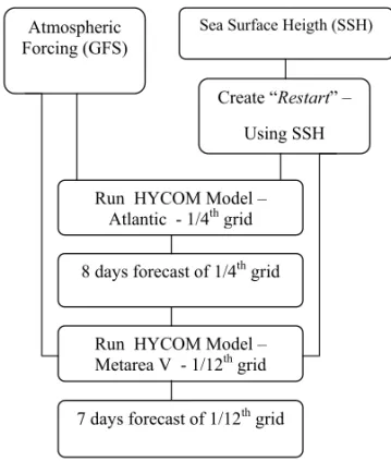
the NRL. Each simulation generated a prediction of eight days for the nesting of the 1/12◦_{grid, spanning from February 1}st ₂₀₁₀ to March 31st_{2010, with outputs every 24 hours.}

Atmospheric Forcing (GFS)

Run HYCOM Model – Atlantic - 1/4th_grid

Sea Surface Heigth (SSH)

Create “ ” – Using SSH

8 days forecast of 1/4th_grid

Run HYCOM Model – Metarea V - 1/12th_grid

7 days forecast of 1/12th_grid

Figure 2 – Scheme of the experiments performed. Observational data

To verify the model results, observed daily data of temperature and salinity were used. They were collected by Argo profilers for the period of February and March 2010. These sources were

taken from the database of the US National Oceanic and At-mospheric Administration – NOAA (http://dapper.pmel.noaa.gov/ dchart) adding up to a total of 804 profiles distributed in the 1/12◦

grid, as shown in Figure 3.

The Argo drifters are equipped with sensors with an accuracy of 0.005◦_{C for temperature, 5 dbar for pressure and 0.01 for}

salin-ity. The temperature and pressure sensors are sturdy and maintain this accuracy when they are calibrated for the entire lifetime of the drifter (which is estimated as 4 years). However, the conductivity sensor, from which salinity is derived, is highly sensitive and is subject to biological encrustations, which may cause fluctuations in its measures (Freeland, 1997; Sall’ee & Morrow, 2007).

On this dataset, quality control was performed on the tem-perature and salinity data, where profiles with excessive de-viations (spikes), distributed outside the climatological stan-dards, excessive gradients and profiles with constant values were corrected or eliminated, following the methodology of The Global Temperature and Salinity Profile Program (GTSPP – http://www.nodc.noaa.gov/GTSPP/gtspp-home.html). Finally, 747 qualified profiles of temperature and salinity were interpo-lated to the vertical levels of the Levitus (1982) climatology. The results of the model were also interpolated to the same levels.

Statistical tools for analysis

For comparison of the Argo temperature (T) and salinity (S) pro-files with the respective propro-files from the numerical experiments, some statistical tools were used: mean, standard deviation (Eq. 1), centered root mean square error (Eq. 2) and correlation (Eq. 3). Due to the great variability of the hydrographic properties of the study area, an option was made to calculate both the standard deviation of the variable (T, S) and also the standard deviation of the difference between the parameters observed and those mod-eled. These analyses showed that in spite of the difference among the profiles in the study area, the difference between the data from the model and data observed displayed similar behavior. Thus, it was opted to make a statistical analysis of the entire water col-umn, the mixed layer and thermocline, where the greatest devia-tions occurred. In this way it is possible to study both the varia-tion of temperature and salinity and the variavaria-tion of the difference between the results of the model and the Argo results.

std = r 1 N X (x − ˉx)2 (1) rms = s P

[(xobs− ˉxobs− (xmod− ˉxmod)]2

(5)

“main” — 2014/1/16 — 15:48 — page 247 — #5

247

Figure 3 – Study area with the positions of the Argo drifters during the months of February and March 2010. The gray

line marks the 200 m depth line.

cor = P

[(xobs− ˉxobs∗ (xmod− ˉxmod)] qP (xobs− ˉxobs)2 N ∗ qP (xmod− ˉxmod)2 N (3)

where_{x is the analyzed variable.}

This work also made use of Taylor diagrams (Taylor, 2001), which provide a concise summary of the statistics, setting out standards of correspondence between a set of reference data and another set to be evaluated. This diagram considers the correla-tion coefficient, the, centered root mean square error, and stan-dard deviation (COR, RMS and STD) for datasets with the same number of samples.

The reference set, represented in this study by the Argo data, produces in relation to itself a self-correlation equal to 1, RMS equal to 0, and the standard deviation varies according to the data sampled. The other set represents the statistical relationship between the observed data and the result of an experiment.

RESULTS

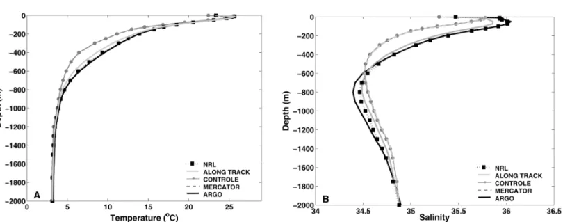
The average vertical profiles of temperature and salinity for each experiment compared with the Argo profiles are presented below. In Figure 4a, which represents the average temperature profile, we may note that from the surface to a depth of approximately 100 meters and less then 900 meters, all the experiments dis-play behavior similar to the observed data. The mean profiles of the 24 h forecasts from the NRL and ALONG-TRACK experiments were closer to the Argo profile than the other forecasts. The maxi-mum difference in temperature (1T) found was 0.5◦_{C and 1.0}◦_C,

respectively. In the region of the thermocline, the MERCATOR and CONTROL profiles display similar values, although with a discrepancy of up to 3.0◦_{C in relation to the observed values.}

These differences are associated to the great variations of tem-perature and salinity that occur in the region and the difficulty of

(6)

Figure 4 – Average profile of a) Temperature and b) Salinity for the entire area for the NRL, ALONG TRACK, MERCATOR and CONTROL experiments and Argo.

representing this variation using only an interpolation at the Levitus levels (1982). Furthermore, the SSH field obtained for MERCATOR has lower spatial resolution that the NRL and ALONG TRACK fields, showing an adjustment less refined in re-lation to the observed data.

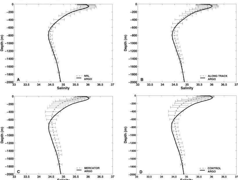
The average profiles of salinity are presented in Figure 4b. Once again, the NRL and ALONG TRACK experiments are those most similar to the observed data. From the surface to 600 meters depth, the NRL has salinity very close to the Argo profile, with a difference of salinity (1S) of less than 0.07. The ALONG TRACK produced salinity slightly below the Argo (1S<0.2). The MER-CATOR and CONTROL experiments, meanwhile, show 1S be-tween 0.6 and 0.7. At depths greater than 600 meters, all the experiments show salinity greater than the observed data, al-though the NRL continues to be the closest to the Argo profile (1S>–0.07).

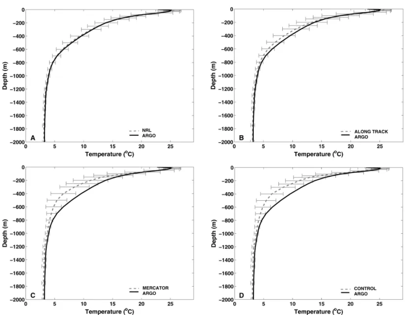
Figure 5 presents, in addition to the observed and modeled average temperature, the standard deviation of difference of tem-perature (std(1T)) of each experiment with respect to the Argo data. The NRL shows the lowest values of std(1T), i.e., besides the average temperature for the entire area being similar, the dif-ference between the profiles of each NRL station and the Argo data is less than in the other experiments in the entire water column, between 0.2◦_{C and 2.4}◦_{C (Fig. 5a, Table 1). The ALONG TRACK,}

MERCATOR and CONTROL experiments (Figs. 5b, 5c and 5d) present a standard deviation varying between 0.3◦_{C and 3.2}◦_C,

0.2◦_{C and 3.4}◦_{C and 0.3}◦_{C and 2.9}◦_{C, respectively, with the}

greatest deviations taking place between 75 and 125 meters. Figure 6 shows the observed and modeled average salinity and standard deviation of the difference of salinity (std(1S)) of

each experiment with respect to the Argo data. The std(1S) from the NRL encompasses the Argo values and the lowest values are at the surface, increasing with depth, between 0 and 0.4 (Fig. 6a, Table 2). The ALONG TRACK also produced a profile similar to the Argo profile (Fig. 6b) and encompasses the entire average of the Argo data. The MERCATOR and CONTROL experiments (Figs. 6c and 6d), meanwhile, besides presenting the values furthest from the Argo average, also present the greatest values of stan-dard deviation with 0.5◦_{C (Table 2), and at some levels do not}

encompass the values of the averages of the Argo data.

Another form of evaluation and comparison between the re-sults of the experiments and the data observed is the Taylor Dia-gram (Fig. 7). As described above, this represents in summarized form the degree of correspondence between the numerical results and the data observed.

Due to the differences observed in the vertical profiles be-tween the mixed layer and the thermocline, it was deemed neces-sary to verify the behavior of temperature and salinity in the Taylor Diagram for these layers separately. The limiting depths were cho-sen based on the similarities of the average vertical distributions of temperature: 0-100 m and 125-800 m.

Figure 7 shows the Taylor diagrams of temperature and salin-ity for the entire water column (A and D), for mixed layer (B and E) and thermocline (C and F). The correlation coefficient is rep-resented by dotted and dashed blue lines. Standard deviation is indicated by black dotted lines. The green dashed lines measure the distance between the point of reference and the analyzed point, representing the RMS.

All the diagrams present 5 points, where A represents the Argo data, which displays a self-correlation equal to 1, RMS equal

(7)

“main” — 2014/1/16 — 15:48 — page 249 — #7

249

Figure 5 – Average temperature profile (◦_{C) from observations and model and standard deviation of the difference for the experiments: (a) NRL, (b) ALONG TRACK,}

(c) MERCATOR and (d) CONTROL.

to 0 and standard deviation of the set of data analyzed. The other points (B, C, D and E) represent the statistical relationship be-tween the data observed (point A) and the result of each one of the experiments, as indicated in the figure.

In the Taylor Diagrams of temperature for the entire water col-umn (Fig. 7a) we observe that the four experiments display values relatively close to the Argo set, for correlation, standard deviation and also RMS. The experiment that displays the best statistical relation to the data observed is the NRL. This experiment has greater correlation (0.99) and lower RMS (0.99◦_{C). While not}

attaining the closest standard deviation to the Argo data, they do have similar values: 8.76◦_{C and 8.67}◦_{C respectively,}

show-ing that both have a very close dispersion from the set. The ALONG TRACK has a high correlation (0.98) and low RMS (1.39◦_{C) in relation to the data. The standard deviation of}

temper-ature (8.80◦_{C) is greater than the NRL. The MERCATOR,}

mean-while, displays the standard deviation closest to Argo (8.68◦_C),

high correlation (0.98) although with a higher RMS (1.58◦_{C). The}

CONTROL displayed a correlation of 0.98, deviation of 8.55◦_C

and error of 1.47◦_{C. Thus, considering the entire water}

col-umn, we note that the imposition of external SSH data improves the results of the forecast, but does not produce a great difference in the statistics.

In the mixed layer, the Taylor Diagram of temperature (Fig. 7b) shows that the NRL best represents the Argo data, dis-playing greater correlation (0.97), and a lower RMS (1.28◦_C).

The STD calculated was very close to the Argo data, 5.23◦_C

and 5.27◦_{C, respectively. Meanwhile the ALONG TRACK and}

MERCATOR experiments showed a correlation equal to 0.94; RMS of 1.78◦_{C and 1.71}◦_{C; and STD of 5.07}◦_{C and 5.00}◦_C,

whereas the CONTROL presented a correlation of 0.95; RMS of 1.61◦_{C and STD of 5.14}◦_{C, showing that the CONTROL is closer}

to the observed data than the ALONG TRACK and MERCATOR experiments.

(8)

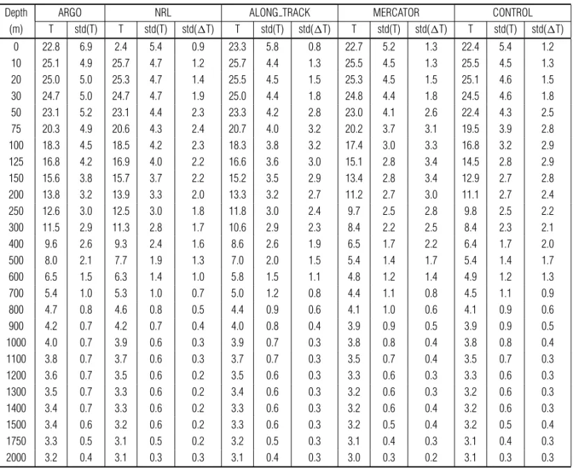
Table 1 – Average of Temperature (T), standard deviation of temperature (std(T)), standard deviation of difference of temperature (std(1T) for the Argo data and the

NRL, ALONG TRACK, MERCATOR and CONTROL experiments at each level. Unit is◦_C.

Depth ARGO NRL ALONG TRACK MERCATOR CONTROL (m) T std(T) T std(T) std(1T) T std(T) std(1T) T std(T) std(1T) T std(T) std(1T) 0 22.8 6.9 2.4 5.4 0.9 23.3 5.8 0.8 22.7 5.2 1.3 22.4 5.4 1.2 10 25.1 4.9 25.7 4.7 1.2 25.7 4.4 1.3 25.5 4.5 1.3 25.5 4.5 1.3 20 25.0 5.0 25.3 4.7 1.4 25.5 4.5 1.5 25.3 4.5 1.5 25.1 4.6 1.5 30 24.7 5.0 24.7 4.7 1.9 25.0 4.4 1.8 24.8 4.4 1.8 24.5 4.6 1.8 50 23.1 5.2 23.1 4.4 2.3 23.3 4.2 2.8 23.0 4.1 2.6 22.4 4.3 2.5 75 20.3 4.9 20.6 4.3 2.4 20.7 4.0 3.2 20.2 3.7 3.1 19.5 3.9 2.8 100 18.3 4.5 18.5 4.2 2.3 18.3 3.8 3.2 17.4 3.0 3.3 16.8 3.2 2.9 125 16.8 4.2 16.9 4.0 2.2 16.6 3.6 3.0 15.1 2.8 3.4 14.5 2.8 2.9 150 15.6 3.8 15.7 3.7 2.2 15.2 3.5 2.9 13.4 2.8 3.4 12.9 2.7 2.8 200 13.8 3.2 13.9 3.3 2.0 13.3 3.2 2.7 11.2 2.7 3.0 11.1 2.7 2.4 250 12.6 3.0 12.5 3.0 1.8 11.8 3.0 2.4 9.7 2.5 2.8 9.8 2.5 2.2 300 11.5 2.9 11.3 2.8 1.7 10.6 2.9 2.3 8.4 2.2 2.5 8.4 2.3 2.1 400 9.6 2.6 9.3 2.4 1.6 8.6 2.6 1.9 6.5 1.7 2.2 6.4 1.7 2.0 500 8.0 2.1 7.7 1.9 1.3 7.0 2.0 1.5 5.4 1.4 1.7 5.4 1.4 1.7 600 6.5 1.5 6.3 1.4 1.0 5.8 1.5 1.1 4.8 1.2 1.4 4.9 1.2 1.3 700 5.4 1.0 5.3 1.0 0.7 5.0 1.2 0.8 4.4 1.1 0.8 4.5 1.1 0.9 800 4.7 0.8 4.6 0.8 0.5 4.4 0.9 0.6 4.1 1.0 0.6 4.1 0.9 0.6 900 4.2 0.7 4.2 0.7 0.4 4.0 0.8 0.4 3.9 0.9 0.5 3.9 0.9 0.5 1000 4.0 0.7 3.9 0.6 0.3 3.9 0.7 0.3 3.8 0.8 0.4 3.8 0.8 0.4 1100 3.8 0.7 3.7 0.6 0.3 3.7 0.7 0.3 3.5 0.7 0.4 3.5 0.7 0.3 1200 3.6 0.7 3.5 0.6 0.2 3.5 0.6 0.3 3.3 0.6 0.3 3.3 0.6 0.3 1300 3.5 0.7 3.3 0.6 0.2 3.4 0.6 0.3 3.2 0.6 0.3 3.2 0.6 0.3 1400 3.4 0.7 3.3 0.6 0.2 3.3 0.6 0.3 3.2 0.6 0.4 3.2 0.6 0.3 1500 3.4 0.6 3.2 0.6 0.2 3.3 0.6 0.3 3.2 0.5 0.4 3.2 0.5 0.4 1750 3.3 0.5 3.1 0.5 0.2 3.2 0.5 0.3 3.1 0.4 0.3 3.1 0.4 0.3 2000 3.2 0.4 3.1 0.3 0.3 3.1 0.4 0.3 3.0 0.3 0.2 3.1 0.3 0.3

In the Taylor Diagram of temperature for the thermocline (Fig. 7c), the NRL also presented better results: greater correla-tion (0.98), lower RMS (1.05◦_{C) and STD very close to the Argo}

data, 4.99◦_{C and 4.84}◦_{C, respectively. The ALONG TRACK and}

CONTROL showed correlation of 0.96, RMS of 1.44◦_{C; 1.45}◦_C

and STD of 4.95◦_{C. The MERCATOR displayed lower correlation}

(0.954), greater RMS (1.58◦_{C) and STD of 4.31}◦_{C, and thus this}

was the experiment with worst results in this region.

The Taylor Diagram of salinity for the entire water column (Fig. 7d) displays greater spread, showing that there is a greater discrepancy in the prediction of salinity. In this case also, the experiment that best represents the observed data is the NRL, with the greatest correlation (0.95) and the smallest RMS (0.24), also displaying the closest standard deviation (0.76) to the Argo

data (0.79). The ALONG TRACK showed the second-best result, with correlation of 0.92, RMS of 0.31 and STD of 0.74. The MERCATOR and CONTROL displayed results very close, corre-lation of 0.88 and RMS of 0.40 for both, while the STD was 0.57 for the MERCATOR and 0.56 for the CONTROL.

In the mixed layer (Fig. 7e), the best result found in the Tay-lor Diagram of salinity was for the NRL, although the correlations were low. The NRL displayed greater correlation (0.90) and lower RMS (0.34). The NRL also showed the closest STD to the data with values of 0.75 and 0.78, respectively. The ALONG TRACK and MERCATOR experiments had the same correlation (0.87) but RMS of 0.41 and 0.30, respectively. The STD for these experi-ments was 0.82 and 0.64. The CONTROL displayed lower corre-lation (0.85), RMS of 0.41 and STD of 0.63, and thus in the Taylor

(9)

“main” — 2014/1/16 — 15:48 — page 251 — #9

251

Figure 6 – Average salinity profile from observations and model and standard deviation of the difference for the experiments: (a) NRL, (b) ALONG TRACK,

(c) MERCATOR and (d) CONTROL.

Diagram, the ALONG TRACK, MERCATOR and CONTROL occupy the same distance (discrepancy) from the observed data.

The Taylor Diagram of salinity for the Thermocline (Fig. 7f) also showed that the NRL was the closest to the Argo data, with greater correlation (0.92), lower RMS (0.22) and the clos-est STD to the data observed, 0.57 and 0.60 respectively. The ALONG TRACK showed a correlation of 0.89, RMS of 0.28 and STD of 0.54, proving to produce the second best forecast. The MERCATOR displayed a result very similar to the CONTROL; cor-relation of 0.79 and 0.80, RMS of 0.41 for both and STD of 0.30 for both.

Thus, in general terms, the Taylor Diagrams for the mixed layer and thermocline displayed the same characteristics as the Taylor Diagram for the entire water column, although with lower values of correlation and greater RMS. This is due to the greater variability of temperature and salinity in the upper layers and the difficulty of the models to reproduce these variabilities of meso and large scale, such as exchange of heat between ocean and

atmosphere, mass exchange between the isopycnal layers, vor-tices, among others. The imposition of SSH, in this study using the Cooper & Haines (1996) method, is used to insert these data into the model. Moreover, the Taylor Diagram for the thermocline displays better results than for the mixed layer, as the Cooper & Haines method does not directly affect the mixed layer.

CONCLUSION

From analysis of the average vertical profiles of T and S and the Taylor Diagrams, it was found that the forecasts from the NRL ex-periment, with initial condition constrained by data from the NRL HYCOM+NCODA+GLOBAL 1/12◦_{, is the one that best represents}

the actual state of the ocean in comparison to the other experi-ments, according to the observational data. This experiment may have presented this result due to the higher-resolution of the SSH data imposed (1/12◦_{), in comparison with the data used in the}

(10)

Figure 7 – Taylor Diagrams: a) Temperature (◦_{C) for the entire water column, b) Temperature of the mixed layer, c) Temperature of the thermocline, d) Salinity}

(11)

“main” — 2014/1/16 — 15:48 — page 253 — #11

253

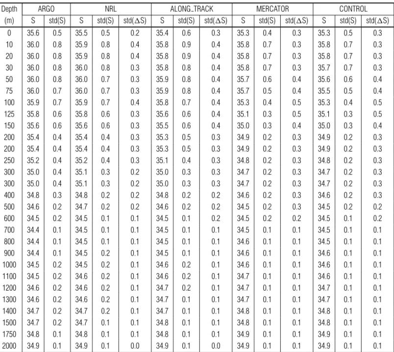
Table 2 – Average of Salinity (S), standard deviation of salinity (std(S)), standard deviation of difference of salinity (std(1S) for the Argo data and the NRL, ALONG TRACK, MERCATOR and CONTROL experiments at each level.

Depth ARGO NRL ALONG TRACK MERCATOR CONTROL (m) S std(S) S std(S) std(1S) S std(S) std(1S) S std(S) std(1S) S std(S) std(1S) 0 35.6 0.5 35.5 0.5 0.2 35.4 0.6 0.3 35.3 0.4 0.3 35.3 0.5 0.3 10 36.0 0.8 35.9 0.8 0.4 35.8 0.9 0.4 35.8 0.7 0.3 35.8 0.7 0.3 20 36.0 0.8 35.9 0.8 0.4 35.8 0.9 0.4 35.8 0.7 0.3 35.8 0.7 0.3 30 36.0 0.8 36.0 0.8 0.3 35.8 0.8 0.4 35.8 0.7 0.3 35.7 0.7 0.3 50 36.0 0.8 36.0 0.7 0.3 35.9 0.8 0.4 35.7 0.6 0.4 35.6 0.6 0.4 75 36.0 0.7 36.0 0.7 0.3 35.9 0.8 0.4 35.7 0.5 0.4 35.5 0.5 0.4 100 35.9 0.7 35.9 0.7 0.4 35.8 0.7 0.4 35.3 0.4 0.5 35.3 0.4 0.5 125 35.8 0.6 35.8 0.6 0.3 35.6 0.6 0.4 35.1 0.3 0.5 35.1 0.3 0.5 150 35.6 0.6 35.6 0.6 0.3 35.5 0.6 0.4 35.0 0.3 0.4 35.0 0.3 0.4 200 35.4 0.4 35.4 0.4 0.3 35.3 0.5 0.3 34.9 0.2 0.3 34.9 0.2 0.3 200 35.4 0.4 35.4 0.4 0.3 35.3 0.5 0.3 34.9 0.2 0.3 34.9 0.2 0.3 250 35.2 0.4 35.2 0.4 0.3 35.1 0.4 0.3 34.8 0.2 0.3 34.8 0.2 0.3 300 35.0 0.4 35.1 0.3 0.2 35.0 0.3 0.3 34.7 0.2 0.3 34.7 0.2 0.3 300 35.0 0.4 35.1 0.3 0.2 35.0 0.3 0.3 34.7 0.2 0.3 34.7 0.2 0.3 400 34.8 0.3 34.8 0.2 0.2 34.8 0.2 0.2 34.6 0.2 0.3 34.6 0.2 0.3 500 34.6 0.2 34.7 0.2 0.2 34.6 0.2 0.2 34.5 0.2 0.3 34.5 0.2 0.2 600 34.5 0.2 34.5 0.1 0.1 34.5 0.1 0.2 34.5 0.2 0.2 34.5 0.1 0.2 700 34.4 0.1 34.5 0.1 0.1 34.5 0.1 0.1 34.5 0.1 0.1 34.5 0.1 0.1 800 34.4 0.1 34.5 0.1 0.1 34.5 0.1 0.1 34.6 0.1 0.1 34.5 0.1 0.1 900 34.4 0.1 34.5 0.2 0.1 34.5 0.1 0.1 34.6 0.1 0.1 34.6 0.1 0.1 1000 34.5 0.2 34.5 0.2 0.1 34.6 0.2 0.1 34.6 0.1 0.1 34.6 0.1 0.1 1100 34.5 0.2 34.6 0.2 0.1 34.6 0.2 0.1 34.7 0.1 0.1 34.6 0.1 0.1 1200 34.6 0.2 34.6 0.2 0.1 34.7 0.2 0.1 34.7 0.1 0.1 34.7 0.1 0.1 1300 34.6 0.2 34.6 0.2 0.1 34.7 0.1 0.1 34.7 0.1 0.1 34.7 0.1 0.1 1400 34.7 0.2 34.7 0.2 0.1 34.7 0.1 0.1 34.8 0.1 0.1 34.8 0.1 0.1 1500 34.7 0.2 34.7 0.1 0.1 34.8 0.1 0.1 34.8 0.1 0.1 34.8 0.1 0.1 1750 34.8 0.1 34.8 0.1 0.1 34.8 0.1 0.1 34.9 0.1 0.1 34.9 0.1 0.1 2000 34.9 0.1 34.9 0.1 0.0 34.9 0.1 0.0 34.9 0.1 0.1 34.9 0.1 0.1

number of data observed from Argo drifters to generate the ex-ternal SSH field, when compared with the SSH data used in the optimal interpolation in the ALONG TRACK. However, it should be noted that SSH data from the NRL HYCOM+NCODA GLOBAL 1/12◦_{were assimilated, and in this article independent}

tempera-ture and salinity profiles were used for comparison. It may also be verified that all the simulations using the Cooper & Haines method with SSH present a better or equal result than those using forecasts without SSH constraint (CONTROL).

Moreover, it was noted that the average profiles show the general behavior of the experiments, although they may oversee regions/layers of great variability, as in the mixed layer. From the Taylor Diagram it was noted that when the deeper layers were

in-cluded in the statistical evaluation, the metrics show better re-sults than the ones in the thermocline and mixed layer for all the experiments. In spite of the great difference of average profiles of temperature in the thermocline, we note through the Taylor Dia-gram there is a high correlation (0.98 to 0.95) between the exper-iments and the Argo data. Furthermore, the RMSs of temperature and salinity found for this region are very close to those found for the entire water column. Thus, based on these statistical analysis one may state that this region is being well represented, especially in the NRL experiment, due to application of the Cooper & Haines method. The mixed layer showed lower correlations because the Cooper & Haines method only imposes an alteration on the thick-ness of the isopycnal layers below this layer.

(12)

Based on these results, a new phase of work will begin, in which SSH data from HYCOM+NCODA will be inserted using the Cooper & Haines method (1996) in the operational system. Other data assimilation methods may also be studied to improve the model results in the mixed layer. One possibility is the use of the Sea Surface Temperature (SST) taken from analysis and/or satel-lite data. A second possibility would be to use vertical profiles or in situ surface data to extrapolate them into its neighboring region on the basis of some interpolation techniques.

ACKNOWLEDGMENTS

This work was supported by PETROBRAS and the Brazilian Oil Regulatory Agency ANP (Agência Nacional de Petróleo, Gás Nat-ural e Biocombust´ıveis), within the special participation research project “Oceanographic Modeling and Observation Network (REMO)”, Cooperation Agreement number 0050.0046200.08.9 between PETROBRAS and the Brazilian Navy.

REFERENCES

BLECK R. 2002. An oceanic general circulation model framed in hybrid isopycnic-Cartesian coordinates. Ocean Modelling, 4: 55–88. CAMPOS EJD. 2006. The Equatorward Translation of the Vitoria Eddy in a Numerical Simulation. Geophysical Research Letters, 33, pp. L22607. DOI: 10.1029/2006GL026997.

CIRANO M, MATA MM, CAMPOS EJD & DEIR Ó NFR. 2006. A circulação oceânica de larga-escala na região oeste do Atlântico Sul com base no modelo de circulação Global OCCAM. Revista Brasileira de Geof´ısica, 24(2): 209–230.

CHASSIGNET EP, SMITH LT, HALLIWELL GR & BLECK R. 2003. North Atlantic simulation with the HYbrid Coordinate Ocean Model (HYCOM): Impact of the vertical coordinate choice, reference density, and thermo-baricity. Journal of Physical Oceanography, 33: 2504–2526.

CHASSIGNET EP, HURLBURT HE, SMEDSTAD OM, HALLIWE GR, WALLCRAFT AJ, METZGER EJ, BLANTON BO, LOZANO C, RAO DB, HOGAN PJ & SRINIVASAN A. 2006. Generalized vertical coordinates for eddy-resolving global and coastal ocean forecasts. Oceanography, 19(1): 118–129.

CHASSIGNET EP, HURLBURT HE, SMEDSTAD OM, HALLIWELL GR, HOGAN PJ, WALLCRAFT AJ, BARAILLE R & BLECK R. 2007. The HYCOM (HYbrid Coordinate Ocean Model) data assimilative system. Journal of Marine Systems, 65: 60–83.

CHASSIGNET EP, HURLBURT HE, METZGER EJ, SMEDSTAD OM, CUMMINGS JA, HALLIWELL GR, BLECK R, BARAILLE R, WALLCRAFT AJ, LOZANO C, TOLMAN HL, SRINIVASAN A, HANKIN S, CORNILLON

P, WEISBERG R, BARTH A, HE R, WERNER F & WILKIN J. 2009. US GO-DAE: Global ocean prediction with the HYbrid Coordinate Ocean Model (HYCOM). Oceanography 22(2): 64–75, doi: 10.5670/oceanog.2009.39. COOPER M & HAINES K. 1996. Altimetric assimilation with water prop-erty conservation. Journal of Geophysical Research, 101: 1059–1077. COUNILLON F & BERTINO L. 2009. Ensemble Optimal Interpolation: multivariate properties in the Gulf of Mexico. Tellus, 61A: 296–308. DOMBROWSKY E, BERTINO L, BRASSINGTON GB, CHASSIGNET EP, DAVIDSON F, HURLBURT HE, KAMACHI M, LEE T, MARTIN MJ, MEI S & TONANI M. 2009. GODAE systems in Operation. Oceanography, 22(3): 80–95.

EZER T & MELLOR GL. 1994. Continuous assimilation of GEOSAT altimeter data into a threedimensional primitive equation Gulf Stream model. J. Phys. Oceanogr., 24(4): 832–847.

EZER T, MELLOR GL, KO D & SIRKES Z. 1993. A comparison of Gulf Stream sea surface height fields derived from Geosat altimeter data and those derived from sea surface temperature data. Journal of Atmospheric and Oceanic Technology, 10: 76–87.

FERNANDES AM, SILVEIRA ICA, CALADO L, CAMPOS EJD & PAIVA AM. 2009. A twolayer approximation to the Brazil Current-Intermediate Western Boundary Current System between 20 S and 28 S. Ocean Modelling, 29: 154–158.

FREELAND H. 1997. Calibration of the conductivity cells on P-ALACE floats. US WOCE Implementation Report, 9: 37–38.

HALLIWELL G. 2004. Evaluation of vertical coordinate and vertical mix-ing algorithms in the Hybrid Coordinate Ocean Model (HYCOM). Ocean Modelling, 7: 285–322.

HOUTEKAMER PL & MITCHELL HL. 1998. Data Assimilation Using an Ensemble Kalman Filter Technique. Mon. Wea. Rev., 126: 796–811. KOURAFALOU VH, PENG G, KANG H, HOGAN PJ, SMEDSTAD O & WEISBERG RH. 2009. Evaluation of Global Ocean Data Assimilation Experiment products on South Florida nested simulations with the Hy-brid Coordinate Ocean Model. Ocean Dynamics, 59: 47–66. DOI: 10.1007/s10236-008-0160-7.

LEVITUS S. 1982. Climatological Atlas of the World Ocean, NOAA. Professional paper, no. 13, U.S. Gov. Printing Office, 173 pp.

MELLOR GL & EZER T. 1991. A Gulf Stream Model and altimetry assim-ilation scheme. J. Geophys. Res., 96(C5): 8779–8795.

OKE PR, SAVOK P & CORNEY SP. 2007. Impacts of localization in the EnKF and EnOI: experiments with a small model. Ocean Dynamics, 57: 32–45. DOI: 10.1007/s10236-006-0088-8.

OKE PR, BRASSINGTON GB, GRIFFIN DA & SCHILLER A. 2010. Ocean data assimilation: a case for ensemble optimal interpolation. Australian Meteorological and Oceanographic Journal, 59: 67–76.

(13)

“main” — 2014/1/16 — 15:48 — page 255 — #13

255

SALL’EE JB & MORROW R. 2007. Delayed mode salinity quality con-trol of Southern Ocean Argo floats. LEGOS technical report, N. 01/2007. LEGOS, Toulouse, France.

SARACENO M, D’ONOFRIO EE, FIORE ME & GRISMEYER WH. 2010. Tide model comparison over the Southwestern Atlantic Shelf, Continen-tal Shelf Research, Volume 30, Pages 1865-1875, ISSN 0278-4343, DOI: 10.1016/j.csr.2010.08.014.

TANAJURA CAS & BELYAEV KP. 2002. On the oceanic impact of a data-assimilation method in a coupled ocean-land-atmosphere model. Ocean

Dynamics, 52: 123–132, DOI: 10.1007/s10236-002-0013-8.

TANAJURA CAS, COSTA FB, RAMOS DA SILVA R, RUGGIERO GA & DAHER VB. 2013. Assimilation of sea surface height anomalies into HYCOM with an Optimal Interpolation scheme over the Atlantic Ocean Metarea V. Revista Brasileira de Geof´ısica, 31(2): 257–270.

TAYLOR KE. 2001. Summarizing multiple aspects of model perfor-mance in a single diagram. J. Geophys. Res., 106: 7183–7192 (PCMDI Report 55).

Recebido em 4 abril, 2012 / Aceito em 26 abril, 2013 Received on April 4, 2012 / Accepted on April 26, 2013

NOTES ABOUT THE AUTHORS

Raquel Leite Mello. Holds a degree in Physics from the Universidade Federal do Rio de Janeiro (UFRJ) (2000), a master’s (2003) and Doctorate (2007) in Physical

Oceanography at the Instituto Oceanográfico, Universidade de São Paulo (IO/USP). Acts in the area of Operational Oceanography in the Rede de Modelagem e Observação Oceanográfica (REMO) at the Centro de Hidrografia da Marinha – Diretoria de Hidrografia e Navegação (CHM-DHN), Niterói – Rio de Janeiro. Experienced in the area of Oceanography, active principally on the following themes: Estuaries, Mid and Large Scale, Oceanography and Numerical Modeling.

Ana Cristina Neves de Freitas. Holds a degree in Oceanology and master’s in Physical, Chemical and Geological Oceanography from the Universidade Federal do

Rio Grande (FURG) (2003). Possesses experience in the area of Physical Oceanography, with emphasis on the analysis, treatment and interpretation of oceanographic data and numerical modeling, with interest in the circulation of the Southwestern Atlantic. Since 2009 active as a researcher in the area of Operational Oceanography in the Rede de Modelagem e Observação Oceanográfica (REMO) at the Centro de Hidrografia da Marinha – Diretoria de Hidrografia e Navegação (CHM-DHN).

Lucimara Russo. Holds a degree in Mathematics from the Universidade Estadual Paulista J´ulio de Mesquita Filho (UNESP) (2005) and a master’s in Meteorology

from the Centro de Previsão de Tempo e Estudos Climáticos at the Instituto Nacional de Pesquisas Espaciais (CPTEC/INPE) (2009). Active in the area of Operational Oceanography in the Rede de Modelagem e Observação Oceanográfica (REMO) at the Centro de Hidrografia da Marinha – Diretoria de Hidrografia e Navegação (CHM-DHN), Niterói – Rio de Janeiro. Is experienced in the area of Meteorology, acting principally in the following themes: Ocean – Atmosphere Interaction, Operational Oceanography and Numerical Modeling.

Jean Felix de Oliveira. Holds a degree in Naval Sciences from the Escola Naval (1993). Specialization in Hydrography for Officers of the Brazilian Navy from

the Diretoria de Hidrografia e Navegação (1996) and a doctorate in Computational Modeling from the Laboratório Nacional de Computação Cient´ıfica (2009). Former Officer-in-Charge of the Oceanographic Modeling Section of the Centro de Hidrografia da Marinha. Active mainly on the following themes: Data Assimilation, HYCOM, Oceanographic Modeling.

Clemente Augusto Souza Tanajura is mechanical-nuclear engineer with Ph.D. in Meteorology by the Center for Ocean-Land-Atmosphere Studies (COLA), University

of Maryland, College Park, US. He was Associate Researcher for the Brazilian National Laboratory for Scientific Computing (LNCC) for 18 years and today he is a Professor for the Federal University of Bahia. Was the scientific-technological coordinator of the Oceanographic Modeling and Observation Network (REMO) from December 2008 until March 2013 and he is a member of the GODAE OceanView Science Team. Works with data assimilation, ocean and atmosphere modeling, short-range weather and ocean predictability and climate studies.

Jo˜ao Bosco Rodrigues Alvarenga. Holds a degree in Naval Sciences from the Escola Naval (1976). Specialization in Hydrography for Officers of the Brazilian Navy

from the Diretoria de Hidrografia e Navegação (1980) and a master’s in Physical Oceanography from the Universidade de São Paulo (1993). Currently is the scientific head of the Rede de Modelagem e Observação Oceanográfica (REMO) at the Centro de Hidrografia da Marinha – Diretoria de Hidrografia e Navegação (CHM-DHN).