The mixed capacitated arc routing problem with non-overlapping routes

Repositório ISCTE-IUL

Deposited in Repositório ISCTE-IUL:

2019-03-27

Deposited version:

Pre-print

Peer-review status of attached file:

Unreviewed

Citation for published item:

Constantino, M., Gouveia, L., Mourão, M. C. & Nunes, A. C. (2015). The mixed capacitated arc routing problem with non-overlapping routes. European Journal of Operational Research. 244 (2), 445-456

Further information on publisher's website:

10.1016/j.ejor.2015.01.042

Publisher's copyright statement:

This is the peer reviewed version of the following article: Constantino, M., Gouveia, L., Mourão, M. C. & Nunes, A. C. (2015). The mixed capacitated arc routing problem with non-overlapping routes. European Journal of Operational Research. 244 (2), 445-456, which has been published in final form at https://dx.doi.org/10.1016/j.ejor.2015.01.042. This article may be used for non-commercial purposes in accordance with the Publisher's Terms and Conditions for self-archiving.

Use policy

Creative Commons CC BY 4.0

The full-text may be used and/or reproduced, and given to third parties in any format or medium, without prior permission or charge, for personal research or study, educational, or not-for-profit purposes provided that:

• a full bibliographic reference is made to the original source • a link is made to the metadata record in the Repository • the full-text is not changed in any way

The full-text must not be sold in any format or medium without the formal permission of the copyright holders. Serviços de Informação e Documentação, Instituto Universitário de Lisboa (ISCTE-IUL)

The mixed capacitated arc routing problem with

non-overlapping routes

Miguel Constantinoa,d, Lu´ıs Gouveiaa,d, Maria Cˆandida Mour˜aob,d, Ana Catarina Nunesc,d,∗

a_{Faculdade de Ciˆencias, ULisboa, 1749-016 Lisboa, Portugal}

b_{Instituto Superior de Economia e Gest˜ao, ULisboa, Rua do Quelhas 6, 1200-781 Lisboa,}

Portugal

c_{ISCTE-IUL – Instituto Universit´ario de Lisboa, Av. das For¸cas Armadas, 1649-026}

Lisboa, Portugal

d_{Centro de Investiga¸c˜ao Operacional, ULisboa, 1749-016 Lisboa, Portugal}

Abstract

Real world applications for vehicle collection or delivery along streets usually lead to arc routing problems, with additional and complicating constraints. In this paper we focus on arc routing with an additional constraint to identify vehicle service routes with a limited number of shared nodes, i.e. vehicle service routes with a limited number of intersections. This constraint leads to solutions that are better shaped for real application purposes. We propose a new problem, the bounded overlapping MCARP (BCARP), which is defined as the mixed capacitated arc routing problem (MCARP) with an additional constraint imposing an upper bound on the number of nodes that are common to different routes. The best feasible upper bound is obtained from a modified MCARP in which the minimization criteria is given by the overlapping of the routes. We show how to compute this bound by solving a simpler problem. To obtain feasible solutions for the bigger instances of the BCARP heuristics are also proposed. Computational results taken from two well known instance sets show that, with only a small increase in total time traveled, the model BCARP produces solutions that are more attractive to implement in practice than those produced by the MCARP model.

∗_{Corresponding author}

Email addresses: mfconstantino@fc.ul.pt (Miguel Constantino),

legouveia@fc.ul.pt (Lu´ıs Gouveia), cmourao@iseg.ulisboa.pt

Keywords: Routing, Integer linear programming, Heuristics, District design, Capacitated arc routing

1. Introduction

Capacitated arc routing mathematical models are often used to formulate delivering or collecting problems where the demands are associated with the links of the underlying network.

There are many variants of these problems. In the typical capacitated arc routing problem (CARP) the objective is to identify minimum cost (or time) routes to be traversed by the vehicles of a given fleet to perform the service in the streets of a network, starting and ending at a depot. The street segments demanding for service are called tasks, and have a given demand to be satisfied by one of the vehicles. The fleet is homogeneous, and the vehicles capacity must be respected.

The CARP was introduced by Golden and Wong (1981), and originally defined on undirected graphs. Since then, several CARP variations and gen-eralizations have been reported in the literature, many of them motivated by real life applications, like waste collection, postal distribution or winter gritting. Dror (2000), Wøhlk (2008), and Corber´an and Prins (2010) survey the research on the CARP and its variations, as well as their applications.

The Mixed CARP (MCARP) generalizes the CARP for mixed graphs, that is, graphs with arcs and edges. The MCARP is more suited to situations where the direction of the traversals has to be taken into account. This is the case of household waste collection (see e.g. Ghiani et al. (2005); Mour˜ao and Amado (2005); Belenguer et al. (2006); Bautista et al. (2008); Mour˜ao et al. (2009); Gouveia et al. (2010)), or road network maintenance (see e.g. Amaya et al. (2007)). The MCARP is NP-hard, since it generalizes the CARP, which is known to be NP-hard (Golden and Wong, 1981).

Since this work is motivated by a refuse collection problem, henceforward the task demands represent the amounts of refuse to collect.

Real world applications often require other constraints that must be added to the basic MCARP model. In some cases, it is not even easy to decide how to measure the additional specifications. Examples of such sit-uations arise when workloads need to be equitably distributed among the vehicles, or different vehicle routes have to be constrained to separated geo-graphical regions. On the recent paper of Ghiani et al. (2014) strategic and

tactical issues involving these type of constraints are surveyed for solid waste management systems.

Also, too many intersections of the service areas of different vehicles can complicate the activities to be held in a region (see e.g., Muyldermans et al. (2002); Mourgaya and Vanderbeck (2007)). According to Kim et al. (2006) and Poot et al. (2002) for instance, solutions with an excessive number of vehicle crossovers tend to be rejected by the practitioners. Kim et al. (2006) also remark that the overlapping of service areas is strongly related to the intersection of the vehicle routes. The number of intersections may decrease if each vehicle service area is concentrated in a geographical region.

An adequate definition of these “nice” regions (sets of arcs and edges) is not easy to state since besides needing to be separated and workload bal-anced, their shape should have other “nice” characteristics. These, apart from being subjective, also allow practitioners to accept or reject a solution after a single viewing. A survey on measures used in the literature for the classification of the regions is provided later in Section 2.

Two of these “attractive” characteristics for the service areas are: i)

con-nectivity and ii) compactness. While concon-nectivity can be clearly defined as

the possibility of traveling between any two points of a region without leaving it, there are different measures of the compactness of a region (MacEachren, 1985). In general, these measures compare the region against an “ideal com-pact shape”, such as a circle or a square, or they are based on the distances between points in the region – higher distances mean, in general, less compact regions.

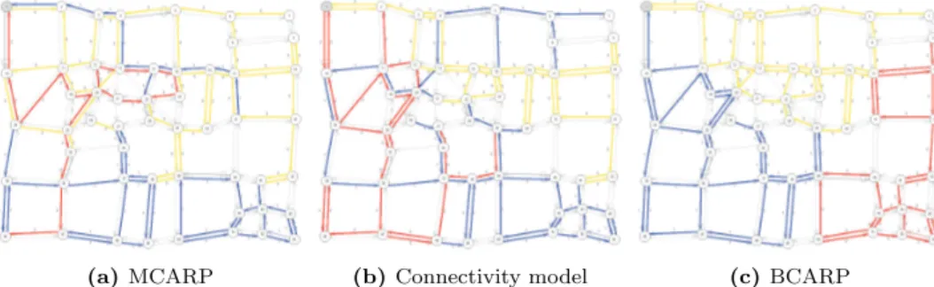
Typical solutions for MCARP models are usually very unsatisfactory in terms of the above criteria. Figure 1a) depicts the optimal MCARP solution for instance lpra2 (see Section 6.1 for a description of the data set), where we can see the overlap of several different vehicle routes (identified by a different color) and very irregular (thus, not “nice”) regions served by each route. Furthermore, we even observe disconnected sequences of tasks within each vehicle service. Thus, solutions resulting from solving the “pure” MCARP can be very inadequate to implement in practice.

The disconnected components observed in the MCARP solutions has mo-tivated our first attempt to improve the shape characteristics of the routes. In this approach, we have imposed constraints guaranteeing that the set of tasks within each route are connected. We omit from this paper the details of how we have modeled and implemented this approach. However, we re-fer the reader to Figure 1b), which illustrates the solution for the instance

lpra2 obtained after adding such “connectivity” constraints to the model. It is quite clear that this solution, despite having connected sets of tasks, still exhibits several undesirable situations such as vehicle routes that overlap and spread (being non compact) in the collection zone.

This attempt to model the “nice” features of the routes by adding con-nectivity constraints illustrates what we have mentioned before, namely that it may not be straightforward to measure and describe the “attractiveness” specification of the routes, in a mathematical way.

(a) MCARP (b) Connectivity model (c) BCARP Figure 1: lpra2 instance – optimal solutions for 3 vehicles.

Motivated by this unsuccessful experiment, in this paper we propose, study and test a new model that uses a constraint simpler to formulate and that is based on a different way to measure the non-overlapping of the vehicle routes. We call this new problem the bounded overlapping MCARP (BCARP). The overlapping is measured in terms of the number of nodes that are common to the tasks of different routes.

One motivation for considering this measure is as follows. We may inter-pret the set of these common (shared) nodes as representing the boundaries between the regions served by each route, and their number as the length of the corresponding boundaries. Thus, one way to promote “nice” (disjoint and compact) regions is by limiting the length of their boundaries.

Figure 1c) depicts the optimal BCARP solution for instance lpra2, where we have included the new constraint on non-overlapping routes. It is interest-ing to compare the three solutions in the figure in order to see the advantage of the latest approach, in terms of compactness and separation of the regions served by each route. Moreover, although connectivity was not enforced in the BCARP model, the resulting solution has connected sets of tasks in each route.

characteristics of solutions. While the first one measures the connectivity, the other two try to measure the compactness, as detailed in Section 5.

This paper is organized as follows. After the literature review (Section 2), the relevant notation is presented in Section 3.1. Next, in Section 3.2 we re-view a model for the MCARP from Gouveia et al. (2010) which will be used as a backbone to model the more restrictive version of the MCARP here studied. In Section 3.3 we describe a variant where we want to minimize the num-ber of shared nodes, named as the non overlapping MCARP (NOMCARP). The value of the NOMCARP objective function is then used to define the upper bound for the number of overlapping nodes in the MCARP. In Sec-tion 3.4 we propose a model for the BCARP that is obtained from combining the MCARP model with constraints from the NOMCARP, and a constraint guaranteeing the referred bounded overlapping. Section 4 is devoted to the methodology employed to find feasible solutions for the BCARP. Solutions for small sized instances are obtained by solving the models in sequence as described above. Heuristics are developed and used to obtain solutions for the larger sized instances. The measures introduced to evaluate the solutions (Section 5) precede the computational results. These involve two sets of well known benchmark instances and are presented and analyzed in Section 6, before the conclusions, in Section 7.

2. Literature review

This section reviews the literature on the solution methodologies and the numerical measures used to obtain and evaluate the “nice” attributes for zones, concerning regions partitioning for routing applications.

When partitioning a region in smaller “nice” zones either for arc or node routing applications, three main approaches have been discussed in the lit-erature. In the first approach, the partitioning and the routing problems are sequentially solved, using multi phase methods (Teixeira et al., 2004; Mour˜ao et al., 2009). In the second, the partitioning and the routing are solved to-gether as a whole problem (Kim et al., 2006; Mour˜ao et al., 2009; Ramos and Oliveira, 2011). In the last one, only the partitioning problem is solved. In some cases, the partitioning is solved keeping in mind that the application is an arc routing problem (Muyldermans et al., 2002, 2003; Perrier et al., 2008; Assis et al., 2014) and in others that the application is on a node routing problem (Mourgaya and Vanderbeck, 2007; Lin and Kao, 2008; R´ıos-Mercado

and Fern´andez, 2009; Gonzalez-Ram´ırez et al., 2011; Jarrah and Bard, 2012; Lei et al., 2012; Salazar-Aguilar et al., 2012).

Among the attributes regarded as relevant when designing zones for rout-ing applications we may highlight the compactness, the non-overlapprout-ing, and the connectivity within each zone.

Compactness is one of the most frequently mentioned characteristics, al-though not always clearly defined. Furthermore, the meaning of compactness slightly differs from author to author, being, for instance, associated with: i) zones shapes as close as possible to circles, squares or rectangles (Lin and Kao, 2008; Gonzalez-Ram´ırez et al., 2011; Jarrah and Bard, 2012); ii) geo-graphically or visually compact zones (Perrier et al., 2008; Lei et al., 2012); or iii) the proximity between the demand entities in the same zone (Poot et al., 2002; Muyldermans et al., 2003; Kim et al., 2006; Tang and Miller-Hooks, 2006; R´ıos-Mercado and Fern´andez, 2009; Salazar-Aguilar et al., 2012; Assis et al., 2014).

Several compactness measures have thus been considered in the literature, whether to evaluate the final solutions, to evaluate compactness during the execution of the solution methods, or both. Generically, these measures try to evaluate the proximity between elements belonging to the same zone, as next detailed.

We may find measures based on maximum travel times (Mour˜ao et al., 2009; Gonzalez-Ram´ırez et al., 2011); on maximum Euclidean distances (R´ıos-Mercado and Fern´andez, 2009; Assis et al., 2014); on the sum of the Euclidean distances (Kim et al., 2006; Mourgaya and Vanderbeck, 2007; Salazar-Aguilar et al., 2012); on the averages and standard deviations of distances, or travel times between customers, or to a reference point in a zone (Poot et al., 2002; Tang and Miller-Hooks, 2006; Mour˜ao et al., 2009); on the perimeters of the zones (Lei et al., 2012); or even perimeters and areas of the zones (Lin and Kao, 2008). Jarrah and Bard (2012) define clusters of clients in the plane in such a way that the ratio of the difference between the maximum and the minimum x coordinate and the difference of the maximum and the minimum

y coordinate lies within a given interval. Poot et al. (2002) and Tang and

Miller-Hooks (2006) also consider the average number of customers in a zone which are closer to the reference point of a different zone rather than to its own, representing costumers who are not well positioned. While Poot et al. (2002) reference point refers to the center of gravity, Tang and Miller-Hooks (2006) opt to use the customer closer to this point, named as the median of the tour. Tang and Miller-Hooks (2006) compute the measures based on

network travel times instead of Euclidean distances.

In some cases, these evaluation compactness measures are also embed-ded in the heuristic processes (Kim et al., 2006; Tang and Miller-Hooks, 2006; R´ıos-Mercado and Fern´andez, 2009; Gonzalez-Ram´ırez et al., 2011; Lei et al., 2012; Salazar-Aguilar et al., 2012; Assis et al., 2014). In other cases, authors devise compactness indicators only embedded in the solution meth-ods (Mourgaya and Vanderbeck, 2007; Lin and Kao, 2008). Although not specifically devised for routing application, it is worth to refer compactness measures that compare the region with that of an ideal shape (MacEachren, 1985; Bozkaya et al., 2003).

Non-overlapping may be defined as zones with clear geographical borders (Cattrysse et al., 1997; Muyldermans et al., 2003), from routes overlapping (Poot et al., 2002; Kim et al., 2006; Lu and Dessouky, 2006; Tang and Miller-Hooks, 2006) or boundary crossing points (Lin and Kao, 2008). However, the literature has been scarce on the evaluation of zones overlapping. Poot et al. (2002) and Kim et al. (2006) evaluate the overlapping of the solutions by counting the number of nodes in more than one convex hull of clusters of nodes (each cluster formed by the stops of a route). Lu and Dessouky (2006) define the crossing length percentage of a trip as the sum of the crossed length of all the crossings divided by the total length of the trip. Tang and Miller-Hooks (2006) claim that by minimizing the number of customers closer to the reference point of another tour, they also minimize the overlapping of the tours. In the mathematical model proposed by Lin and Kao (2008), an upper limit for the number of boundary crossing points is imposed, and the number of such points is also used to evaluate the overlapping of the final solutions. These authors consider a predefined set of small land parcels, representing small collection areas regarding the amount of refuse to collect, and with the road lengths per parcel previously computed. The aim is to assign the parcels into balanced regions, regarding the refuse to collect and the road lengths. In the models here proposed no predefined routes or areas are imposed, and the crossing points are determined by the models.

Matis (2008) measures the visual attractiveness of a tour by combining, in only one equation, the number of crossings amongst different routes; the com-pactness (defined from the distances between customers in the same route); and the number of customers in a route which are closer to the center of gravity of another route.

Note that in this paper, the definition of attractive routes does not con-sider the location of the depot (the same applies to the definitions given in

the previous references). This implies that the design and cost of the optimal solutions may be influenced by the time taken traveling from the depot to the first service, and from the last service back to the depot. On the other hand, the alternative approach (incorporating the location of the depot in the definition of attractive routes) may produce lopsided shaped routes or even routes with more odd shapes. A computational study to compare the two approaches may shed some light on the advantages and disadvantages of each approach. Such is the purpose of future work.

Zones contiguity is generally related to the connectivity between all of its demand entities (Muyldermans et al., 2003; Perrier et al., 2008; Assis et al., 2014) or the possibility to reach all of them within the zone (R´ıos-Mercado and Fern´andez, 2009; Salazar-Aguilar et al., 2012).

In this paper, we propose an exact method, based on a model that simul-taneously designs sectors and builds routes, and a heuristic solution method which sequentially solves the two problems. In fact, by solving a MCARP with an upper bound on the number of overlapping areas, we are able to de-sign “nice” routes. These methods may then directly be applied to a sectors design problem, if each sector is assigned to one vehicle.

3. Models

In this section we review and present models for three related problems, i) the MCARP; ii) the non overlapping MCARP (NOMCARP), which also identifies vehicle routes as in the MCARP, but the minimization criteria is on non-overlapping; and iii) the BCARP, which is the MCARP with an additional constraint on the number of overlappings. We also show that the NOMCARP may be solved by a simpler model, with the same objective, but only requiring the allocation of tasks to the vehicle routes (the design of routes is not required). The new and simpler model is called as the non overlapping routes model (nor ).

For simplicity, and without loss of generality, we assume that no demand links are incident into the depot. In the other cases, a dummy depot is considered, only linked with the depot, and from where vehicle routes must start and end, being the depot treated as a common node. We also considered that each zone is served by only one vehicle route.

3.1. Notation

The initial mixed network, (N, AD, AR, ER), includes deadheading, i.e.

links with no demand for service, and required (or demand) links. N is the set of nodes, representing the depot (node s), and street crossings or alleys. All deadheading links are represented by arcs in AD. To identify the links

having a service to be performed, and called required links or tasks, we use the sets AR and ER, corresponding to the set of the required arcs and the

set of required edges, respectively.

For the directed formulations that we will use, we define the directed graph G = (N, A) as next detailed. All links are represented by arcs in

A = AD ∪ R where R = AR∪ AER is the set of required arcs, with AER =

{(i, j), (j, i) : {i, j} ∈ ER∧i < j}. That is, in the directed graph G = (N, A),

each required edge {i, j} ∈ ER is replaced by two opposite arcs, (i, j) and

(j, i), with the same associated data as the original edge. Only one of these two arcs is required to be served. Thus, |R| = |AR| + 2|ER|, and |AR| + |ER|

is the number of tasks.

We assume that both G and its subgraph spanned by N\{s} are strongly connected graphs. For simplicity, all nodes in N\{s} are endpoints of at least one task. Thus, nodes i ̸= s which are not endpoints of a task are removed from the network and connections in the original network using these nodes are reestablished by adding arcs with durations corresponding to shortest deadheading path values in the original network.

The following notation is also needed to describe the models.

• For each link, arc (i, j) or edge {i, j}, dij > 0 is its deadheading time, i.e.,

the time needed to traverse the street without serving it. Additionally, each required link (i, j) or {i, j} has an associated demand, qij > 0, and a

service time, tij ≥ dij.

• A fleet of P identical vehicles is available, each with a capacity of W . The

time needed to empty a vehicle is λ.

• v(.) is the optimal value of model (.) or the value of a feasible solution

obtained with model (.).

3.2. MCARP model

Here, we briefly review the model of Gouveia et al. (2010), named by (mcar ).

Thus, for each route p = 1, . . . , P , let:

• xp

• yp

ij be the number of times that arc (i, j)∈ A is deadheaded by route p. • fp

ij be the flow in arc (i, j) ∈ A, related to (part of) the route demand,

needed to guarantee the routes connectivity.

(mcar ) min P ∑ p=1   ∑ (i,j)∈A dijyijp + ∑ (i,j)∈R tijxpij+ λ ∑ (s,j)∈A yp_sj   (1a) s.t.: P ∑ p=1 xp_ij = 1 ∀(i, j) ∈ AR (1b) P ∑ p=1 ( xp_ij+ xp_ji)= 1 ∀(i, j) ∈ AER: i < j (1c) ∑ j:(i,j)∈A yp_ij+ ∑ j:(i,j)∈R xp_ij = ∑ j:(j,i)∈A yp_ji+ ∑ j:(j,i)∈R xp_ji ∀i ∈ N; ∀p (1d) ∑ (s,j)_∈A y_sjp 6 1 ∀p (1e) ∑ j:(j,i)∈A f_jip − ∑ j:(i,j)∈A f_ijp = ∑ j:(j,i)∈R qjixpji ∀i ∈ N \ {s}; ∀p (1f) ∑ (s,j)∈A f_sjp = ∑ (i,j)∈R qijx p ij ∀p (1g) f_ijp 6 W(yp_ij+ xp_ij) ∀(i, j) ∈ R; ∀p (1h) f_ijp 6 W y_ijp ∀(i, j) ∈ AD;∀p (1i) xp_ij ∈ {0, 1} ∀(i, j) ∈ R; ∀p (1j)

y_ijp > 0 and integer ∀(i, j) ∈ A; ∀p (1k)

f_ijp > 0 ∀(i, j) ∈ A; ∀p (1l)

The objective function (1a) minimizes the total traveling time, given by the deadheading, the service and the dump times. Constraints (1b) and (1c) ensure that all the tasks are served by vehicle routes; (1d) impose the conti-nuity of routes at each node; (1e) are needed to adequately charge the dump cost in the objective function and to ensure that no more than P vehicles are used; (1f) and (1g) are flow conservation constraints, that together with the linking constraints (1h)–(1i) force the connectivity of the routes. Con-straints (1h)–(1i) are also used to guarantee that each route total demand is compatible with the vehicles capacity, W .

symmetry-breaking inequalities similar to the ones suggested in Benavent et al. (2014). However, as no more instances were solved by its inclusion in the models we drooped this additional constraints in the models here proposed.

3.3. Models for the non overlapping MCARP (NOMCARP)

In this subsection we describe two models for the NOMCARP, named as (nomcar ) and (nor ). The objective is to assign tasks (corresponding to arcs or edges) to vehicle routes while minimizing the overlapping. One way to measure this overlapping is by counting the number of routes each end node of a task is assigned to.

3.3.1. Model (nomcar)

For p = 1, . . . , P , and o ∈ N, let np_o be a binary variable, indicating whether node o is an end node of a task assigned to route p. With these variables the expression ∑_p=1,...,P np

o represents the number of routes node o belongs to. Thus, in our models, the summation term (2) represents the

number of routes graph nodes belong to, and is used to measure the overlap-ping. ∑ o∈N P ∑ p=1 np_o (2)

To obtain a model to minimize the overlapping of the vehicle routes, we can replace the objective function (1a) of the MCARP model by the minimization of (2), min ∑ o_∈N P ∑ p=1 np_o (3)

and include the following constraints, which force np

o to be one if node o is

an end node of a task belonging to vehicle route p:

xp_ij 6 npo ∀(i, j) ∈ AR; o = i, j;∀p (4a)

xp_ij+ xp_ji6 np_o ∀(i, j) ∈ AER : i < j ; o = i, j;∀p (4b)

Let us denote by (nomcar ) the model resulting from the (mcar ) model by replacing the objective function (1a) with (3), and including the additional constraints (4a) to (4c).

3.3.2. Model (nor)

We observe that for the new given objective (3) we need no information about the vehicle routes that are used to visit the tasks (this statement will be clarified later on). Hence, we can reformulate and simplify the model as follows.

For p = 1, . . . , P , let zap_ij be a binary variable equal to one iff task (i, j)∈

AR is assigned to vehicle p, and let zepij be a binary variable equal to one

iff task {i, j} ∈ ER is assigned to vehicle p. Thus, variables zapij and ze p ij

correspond, respectively, to xp_ij for (i, j)∈ AR, and to xpij+ x p

ji for{i, j} ∈ ER

in the previous models (mcar ) and (nomcar ). Consider the following model:

(nor ) N O = min ∑ o_∈N P ∑ p=1 np_o (3) s.t.: P ∑ p=1 zap_ij = 1 ∀(i, j) ∈ AR (5a) P ∑ p=1 zep_ij = 1 ∀{i, j} ∈ ER (5b) ∑ (i,j)∈AR qijza p ij+ ∑ {i,j}∈ER qijze p ij 6 W ∀p (5c) zap_ij6 np_o ∀(i, j) ∈ AR; o = i, j;∀p (5d) zep_ij 6 npo ∀{i, j} ∈ ER; o = i, j;∀p (5e) zap_ij∈ {0, 1} ∀(i, j) ∈ AR;∀p (5f) zep_ij ∈ {0, 1} ∀{i, j} ∈ ER;∀p (5g) np_o∈ {0, 1} ∀ o ∈ N; ∀p (4c)

In the (nor ) model the objective function (3) minimizes the number of nodes visits. Constraints (5a) and (5b) assign each task to only one vehicle, and (5c) ensures that this assignment respects the vehicles capacity. Linking constraints (5d) and (5e) are needed to relate the assigned tasks with the task nodes variables.

In order to see that the two models, (nor ) and (nomcar ), are equivalent, we state and prove (see Appendix A) the following result.

Proposition. Given a feasible solution of any one of the models (nor) and (nomcar), there is a feasible solution of the other model, with the same ob-jective value.

3.4. Bounded overlapping MCARP model (bcar)

We can use the optimal value of the problem defined in Subsection 3.3 to define a tight upper bound for the non-overlapping constraint in the model for the BCARP, named as (bcar ). As referred before, the BCARP is a MCARP with a bounded number of overlapping areas.

Besides (1a)–(1l), which are taken from the MCARP model, we add a constraint, (6), imposing the previously mentioned upper bound, N O, on the number of times that the nodes are shared, and the linking constraints between node and routing variables are also needed and stated by (4a)–(4c).

∑ o∈N P ∑ p=1 np_o6 NO (6)

As we will see in the computational results, the MIP solver, within a time limit of one hour, is not able to find feasible solutions for the biggest tested instances with the (bcar ) model. In order to overcome this disadvantage we have developed a heuristic, described in Section 4.

4. Solving BCARP instances

To solve instances of the BCARP we hopefully solve the two models, (nor ) and (bcar) (see Sec. 4.1). However, in situations where the MIP solver does not provide the optimal solution within the prescribed time limit for one of the two models, we use heuristics as detailed in Sections 4.2 and 4.3. In the computational results section, we compare the solutions produced by the heuristic and by the (bcar ) model, when possible.

4.1. Solving the BCARP using models (nor) and (bcar)

In theory, optimal solutions for BCARP instances may be obtained if a MIP solver is sequentially applied to the two models. To solve a given instance, we first solve the corresponding (nor ) model to identify the upper bound on the number of shared nodes, NO. The model (bcar) is then solved.

This methodology, as it will be computationally confirmed in Section 6, only works for small instances, since the MIP solver used (CPLEX) fails to solve (bcar) or even (nor) for medium size instances (from 30/40 nodes, 100/90 links and 11 vehicles for mval instances and from 145 nodes, 360 links and 8 vehicles for lpr instances) within the time limit of one hour. Feasible solutions for the bigger instances are found through the heuristics next detailed.

4.2. Solving (nor)

Whenever the MIP solver fails to solve to optimality or even to find a feasible solution for (nor ) we resort to a heuristic. With that purpose,

P seed-tasks are first selected, chosen far from the depot and from each

other, and assigned to the vehicles. Let vp be the seed-task of vehicle p. A

new objective function which measures the distances between tasks and the seed-tasks is defined. Let distuvp be the undirected distance between task

u = (i, j) ∈ AR or u = {i, j} ∈ ER and the seed-task vp ∈ AR∪ ER, i.e.,

the shortest path deadheading time computed ignoring the orientation of the arcs, and not including du nor dvp. The objective function (3) is replaced by

min P ∑ p=1 ( ∑ u_∈AR distuvpza p u+ ∑ u_∈ER distuvpze p u ) (7)

and a feasible solution to (nor ) is obtained by (7) within constraints (5a), (5b), (5c), (5f) and (5g).

We first observe that this variant of the (nor ), named as (hnor), is easier to solve since we have omitted the variables np

o and the corresponding

con-straints. Moreover, with the fixed seeds and (7) the symmetric assignments of the (nor ) model are avoided. The underlying idea of the new objective is to fix tasks that are close to the seed-tasks.

The optimal solution for (hnor ) is then used as follows: tasks such that the two end-nodes belong to only one vehicle in the (hnor ) solution are fixed to that vehicle, and we then solve a restricted (nor ) with these tasks fixed. By first solving the (hnor ), the restricted (nor) becomes easier to solve (through the fixing of variables – corresponding to task assignments).

The value of N O to be used in the (bcar ) model, and in the 2-phase heuristic described in the next section, is then the best of the following two values: i) the overlapping in the solution described above, computed by (2); ii) the best value obtained by the MIP solver for the (nor ) model.

4.3. A 2-phase Heuristic for the BCARP

A feasible solution for (bcar ) can be obtained by solving a mixed arc routing problem per vehicle, after solving (nor ). In the first phase, model (nor ) is used to obtain an assignment of tasks to vehicles, and then, in the second phase, this assignment is used to build the routes of each vehicle.

Note that each vehicle subproblem is non-capacitated, as (nor ) assigns tasks taking vehicle capacities into account. The resulting subproblems are thus substantially easier to solve than the original MCARP, since the values of the variables for the assignment of tasks to routes are already chosen, except for the direction for servicing the required edges.

In the computational section we compare, whenever possible, the solu-tions obtained by this heuristic with the solusolu-tions obtained with (bcar ).

5. “Nice” solution measures

As referred, “nice” solutions stand for connected and compact solutions. To evaluate the connectivity and the compactness of a solution we propose three measures. We opted for normalized measures as this helps examining and classifying solutions of different characteristics, as well as isolated solu-tions. The proposed measures are designed mainly to evaluate solutions in urban environments. It is often the case in many cities that the geometry of streets is rectangular, and |AD| is small when compared with |AR∪ ER|. • Connectivity Index (CI) is the average number of connected components

(CC) of the set of tasks in the service zones, given by CI = CC

|routes|, where |routes| is the number of routes of the solution under evaluation. In the

“ideal” situation the tasks of each zone are all connected and the value of

CI is equal to one.

• Average Tasks Distance (ATD) is the average of the shortest path

dead-heading times between tasks within service zones, computed by Equa-tion (8), AT D = 1 |routes| P ∑ p=1 ∑ a,b served by p Dab |taskpairs| (8)

where |taskpairs| = |AR∪ER|×(|AR∪ER|−|routes|)

2×|routes|2 represents an approximation for the mean value of the number of task pairs per route, and Dab is the

minimum deadheading time from task a to task b, not including da nor db. These values represent the minimum between at most eight shortest

deadheading travel times, as we are dealing with mixed graphs. In fact, if both a, b∈ ER, eight distances are considered to compute Dab (see Mour˜ao

et al. (2009)), resulting in a symmetric distance matrix D. Note that, “nicer” solutions are obtained with a smaller AT D value. We can observe that routing distances tend to increase when the shape of the service zones deviates from “nice” compact shapes such as circles or squares.

• Routes Overlapping Index (ROI), given by Equation (9), measures the node

overlapping in the solution obtained when compared with the one in an “ideal” solution. Again, smaller values of this index correspond to “nicer” solutions.

ROI =_(√ N O− |N|

|routes| +√|N| − 1)2− |N|

(9)

In Equation (9), N O− |N| is the node overlapping of the solution under evaluation, with N O here computed by (2), while(√|routes| +√|N| − 1

)2 − |N| represents the node overlapping in an “ideal” solution for an hypothetical

instance, as next detailed.

In order to motivate the index ROI, we consider a hypothetical instance with |N| = n2 _{nodes and} |routes| = r2 _{service zones, with n and r integer} and n − 1 multiple of r. Assume further that nodes are placed uniformly in a square in the plane. In the “ideal” partition of this square, each of the |routes| service zones is contained in a smaller square with [1 + (n − 1)/r]2 nodes each (see Figure 2, where n = 13 and r = 3). Most nodes belong to only one of these squares, others belong to two and some belong to four. The sum of the number of squares each node belongs to is given by

|routes|×[1+(n−1)/r]2 _{= (r + n−1)}2_{. Hence, the overlapping is calculated} by (√|routes| +√|N| − 1

)2

− |N|. We use this formula even if the above

assumptions on|N| and |routes| are not satisfied. Observe that no conditions on the tasks are imposed. It may happen that some nodes that belong to more than one square are only visited by one route from a single sector. In order to have it simpler, the definition of the third measure omit these situations. Note that, this simplification does not spoil the “significance” and “information” of the measure.

Table 1 presents the values for the “nice” solution measures, that are used to compare connectivity and compactness for the optimal lpra2

solu-Figure 2: Hypothetical instance and “ideal” solution with |N| = 169 and |routes| = 9. In this case

(√

|routes| +√|N| − 1)2− |N| = 56.

tion (Figure 1) computed with the three models ((mcar), connectivity model, and (bcar)). This instance has 104 tasks and 3 routes are needed. The con-nectivity index, CI, is higher for the MCARP solution, thus indicating a less “nice” solution. The BCARP model, although not explicitly enforcing the connectivity constraints, produces solutions that are, in terms of connectiv-ity, as good as the ones obtained by the connectivity model. We observe a similar behavior concerning the other measures, AT D and ROI; the so-lutions obtained from the MCARP model are always worse than the ones obtained from the connectivity model, which, in turn, are outperformed by the solutions generated by the BCARP model.

Through our computational experiments, we will confirm these results, namely we will see that feasible vehicle routes obtained with the BCARP model are substantially more compact and then more attractive to the users. Table 1: lpra2 instance – characteristics of the optimal solutions.

Connectivity

(mcar) model (bcar) Number of connected components 6.0 3.0 3.0

CI 2.0 1.0 1.0

Number of shared nodes 85.0 78.0 59.0

AT D 98.7 87.6 61.1

ROI 2.9 2.2 0.5

6. Computational results

In this section we describe computational results from the approaches previously proposed and discussed. The results for the MCARP and BCARP models and the heuristic are analyzed and compared under three different

view-points to evaluate the effect of the new overlapping constraint on the routes:

i) The impact on the objective values (total traveling time). ii) The impact on the gap values and CPU times.

iii) The shape of the solutions.

Exact and heuristic approaches are also compared for the BCARP to access the quality of the proposed heuristic, and also to evaluate the size of the instances that can be solved to optimality by the proposed ILP model.

The shape of the solutions is evaluated according to the measures de-scribed in Section 5.

The computational results were obtained with the MIP solver CPLEX 12.5, on a personal computer (Intel Core i7-3520M 2.90GHz processor and 8 GB of RAM, under 64-bit Windows 7 Professional), for two sets of benchmark MCARP instances detailed in Section 6.1. The analysis of the results is provided in Section 6.2.

6.1. Test instances

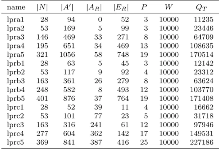
Computational experiments were conducted with the MCARP instances also used in Belenguer et al. (2006) and Gouveia et al. (2010), named lpr and mval. The instances characteristics are displayed in Table 2 and in Table 3. The first column in these tables indicates the instance name, followed by the number of nodes, |N|. Third to fifth columns depict the total number of links, |A′| = |AD| + |AR| + |ER|, the number of required arcs, |AR|, and the

number of required edges, |ER|. The number of vehicles, P , its capacity, W ,

and the total network demand, QT, are shown in the three last columns. In

the 34 mval instances (Table 3) all links have an associated service, and then the total number of links, |A′|, is given by summing the number of arc and edge tasks, |AR| + |ER|.

6.2. Analysis of computational results

Relevant computational results, comparing solution values deviations and CPU times of the methods, are displayed in Table 4 and Table 5, respectively for the mval and for the lpr instances. As before, the first column indicates the instance name.

Table 2: lpr instances characteristics. name |N| |A′| |AR| |ER| P W QT lpra1 28 94 0 52 3 10000 11235 lpra2 53 169 5 99 3 10000 23446 lpra3 146 469 33 271 8 10000 64709 lpra4 195 651 34 469 13 10000 108635 lpra5 321 1056 58 748 19 10000 170514 lprb1 28 63 5 45 3 10000 12142 lprb2 53 117 9 92 4 10000 23312 lprb3 163 361 26 279 8 10000 63624 lprb4 248 582 8 493 12 10000 103770 lprb5 401 876 37 764 19 10000 171408 lprc1 28 52 39 11 4 10000 16662 lprc2 53 101 77 23 5 10000 31718 lprc3 163 316 241 61 12 10000 97946 lprc4 277 604 362 142 17 10000 149531 lprc5 369 841 387 416 25 10000 227186

Table 3: mval instances characteristics.

name |N| |AR| |ER| P W QT name |N| |AR| |ER| P W QT mval1a 24 20 35 4 200 358 mval6a 31 22 47 5 170 451 mval1b 24 13 38 5 120 358 mval6b 31 22 44 6 120 451 mval1c 24 17 36 10 45 358 mval6c 31 23 45 12 50 451 mval2a 24 16 28 4 180 310 mval7a 40 36 50 5 200 559 mval2b 24 12 40 5 120 310 mval7b 40 25 66 6 150 559 mval2c 24 14 35 10 40 310 mval7c 40 28 62 11 65 559 mval3a 24 15 33 4 80 137 mval8a 30 20 76 5 200 566 mval3b 24 16 29 5 50 137 mval8b 30 27 64 6 150 566 mval3c 24 18 25 9 20 137 mval8c 30 28 55 11 65 566 mval4a 41 26 69 5 225 627 mval9a 50 32 100 5 235 654 mval4b 41 19 83 6 170 627 mval9b 50 44 76 6 175 654 mval4c 41 21 82 7 130 627 mval9c 50 42 83 7 140 654 mval4d 41 21 83 11 75 627 mval9d 50 38 93 12 70 654 mval5a 34 22 74 5 220 614 mval10a 50 32 106 5 250 704 mval5b 34 35 56 6 165 614 mval10b 50 33 101 6 190 704 mval5c 34 17 81 7 130 614 mval10c 50 36 100 7 150 704 mval5d 34 29 63 11 75 614 mval10d 50 42 87 12 75 704

i) Evaluating the feasible solution values

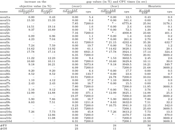
The second column in Tables 4 and 5 give information on the increase in (bcar ) objective value, measured in percentage, from the optimum value of (mcar ), whilst column three depicts the same percentage comparing the solution values of the BCARP heuristic with (mcar ) optimum values. Table 4: Computational results – mval instances.

increase on the gap values (in %) and CPU times (in sec)

objective value (in %) (mcar ) (bcar ) Heuristic

name v(B)−v(F )_{v(F )} H−v(F )_{v(F )} v(F )−LbF_LbF cpu v(B)−LbB_LbB cpu H−LbB_LbB cpu

mval1a 0.00 0.43 0.00 5.4 * 0.00 12.5 0.43 0.3 mval1b 15.33 15.33 0.00 0.4 * 0.00 341.4 0.00 0.5 mval1c – – 7.85 7200.0 * – 6775.8 25.94 3176.1 mval2a 14.51 19.14 0.00 1.6 * 0.00 2.4 4.04 0.1 mval2b 9.37 10.89 0.00 5.7 * 0.00 72.5 1.39 0.4 mval2c – – 7.16 7200.0 * – 4000.8 23.66 401.1 mval3a 6.09 6.96 0.00 1.1 * 0.00 1.4 0.82 0.2 mval3b 4.23 7.04 0.00 5.7 * 0.00 261.9 2.70 0.4 mval3c – – 6.41 7200.0 * 21.15 4232.4 35.26 632.7 mval4a 7.24 7.59 0.00 19.7 * 0.00 73.6 0.32 1.2 mval4b 14.62 14.92 0.00 61.1 * 14.62 3620.1 14.92 20.1 mval4c 17.78 17.14 0.00 6921.3 * 17.78 3924.1 17.14 324.4 mval4d – – 6.35 7200.0 – 7200.0 20.81 3600.2 mval5a 11.22 12.23 0.00 9.4 * 1.53 3602.5 2.45 2.6 mval5b 10.60 10.11 0.00 7200.0 * 10.60 3629.8 10.11 30.0 mval5c 9.18 16.21 0.00 5073.8 * 9.18 3949.5 16.21 349.7 mval5d – – 6.99 7200.0 – 7200.0 21.68 3600.2 mval6a 9.20 9.20 0.00 6.4 * 0.00 17.7 0.00 0.5 mval6b 8.52 8.52 0.00 133.7 * 0.00 22.6 0.00 0.7 mval6c – – 10.91 7200.0 24.78 7200.0 33.04 3600.3 mval7a 1.10 4.12 0.00 57.2 * 1.10 3600.8 4.12 0.9 mval7b 2.43 2.43 0.00 16.7 * 0.00 15.5 0.00 1.0 mval7c – – 7.80 7200.0 – 7200.0 11.95 3600.3 mval8a 5.16 9.12 0.00 9.0 * 0.00 781.1 3.76 1.1 mval8b 12.99 14.88 0.00 371.1 * 12.99 3625.1 14.88 25.3 mval8c – – 19.37 7200.0 – 7200.0 33.89 3600.2 mval9a 5.90 7.86 0.00 16.7 * 5.90 3602.0 7.86 2.2 mval9b 8.83 7.51 0.00 1211.8 * 8.83 3632.0 7.51 32.2 mval9c – – 0.23 7200.0 * 10.75 3941.9 12.15 342.0 mval9d – – 12.85 7200.0 – 7200.1 25.69 3600.5 mval10a 7.26 7.73 0.00 45.8 * 7.26 3613.2 7.73 13.3 mval10b – 12.86 0.00 7200.0 * – 4478.7 12.86 879.0 mval10c – 11.08 0.00 7200.0 – 7200.0 11.08 3600.2 mval10d – – 6.31 7200.0 – 7200.1 23.50 3600.3 #FS 34 24 34 #OS 23 11 4

v(B) = (bcar ) objective value; v(F ) = (mcar ) objective value; H = heuristic value; LbB = (bcar ) lower bound value; LbF = (mcar ) lower bound value;

#FS = number of feasible solutions; #OS = number of optimal solutions;

–: the MIP solver did not find the optimal value of (mcar ) or a feasible solution for (bcar ) within the time limit; *: (nor ) optimally solved by the MIP solver in 1 hour.

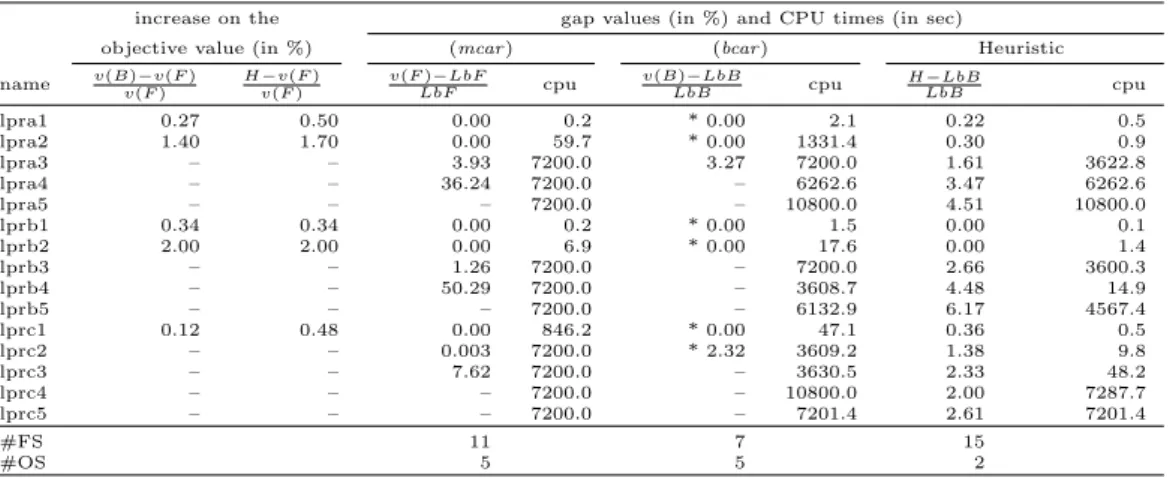
The second column (Tables 4 and 5), shows, as expected, an increase in (bcar ) feasible solution values when compared with (mcar ) optimum values. From the values reported in the third column, we may realize that the heuristic performs better on the lpr instances rather than on the mval ones. In fact, it produces significantly smaller deviations for the lpr. Regarding the increase on the objective values, the behavior of (bcar ) and the heuristic are similar, the latter being able to solve all the instances.

Table 5: Computational results – lpr instances.

increase on the gap values (in %) and CPU times (in sec)

objective value (in %) (mcar ) (bcar ) Heuristic

name v(B)−v(F )_{v(F )} H−v(F )_{v(F )} v(F )−LbF_LbF cpu v(B)−LbB_LbB cpu H−LbB_LbB cpu

lpra1 0.27 0.50 0.00 0.2 * 0.00 2.1 0.22 0.5 lpra2 1.40 1.70 0.00 59.7 * 0.00 1331.4 0.30 0.9 lpra3 – – 3.93 7200.0 3.27 7200.0 1.61 3622.8 lpra4 – – 36.24 7200.0 – 6262.6 3.47 6262.6 lpra5 – – – 7200.0 – 10800.0 4.51 10800.0 lprb1 0.34 0.34 0.00 0.2 * 0.00 1.5 0.00 0.1 lprb2 2.00 2.00 0.00 6.9 * 0.00 17.6 0.00 1.4 lprb3 – – 1.26 7200.0 – 7200.0 2.66 3600.3 lprb4 – – 50.29 7200.0 – 3608.7 4.48 14.9 lprb5 – – – 7200.0 – 6132.9 6.17 4567.4 lprc1 0.12 0.48 0.00 846.2 * 0.00 47.1 0.36 0.5 lprc2 – – 0.003 7200.0 * 2.32 3609.2 1.38 9.8 lprc3 – – 7.62 7200.0 – 3630.5 2.33 48.2 lprc4 – – – 7200.0 – 10800.0 2.00 7287.7 lprc5 – – – 7200.0 – 7201.4 2.61 7201.4 #FS 11 7 15 #OS 5 5 2

v(B) = (bcar ) objective value; v(F ) = (mcar ) objective value; H = heuristic value; LbB = (bcar ) lower bound value; LbF = (mcar ) lower bound value;

#FS = number of feasible solutions; #OS = number of optimal solutions;

–: the MIP solver did not find the optimal value of (mcar ) or a feasible solution for (bcar ) within the time limit; *: (nor ) optimally solved by the MIP solver in 1 hour.

ii) Evaluating the gap values and CPU times

To evaluate the impact of the extra constraints limiting the overlapping, we also compare gap values (in percentage) and CPU times (in seconds) for the MCARP with the ones of the two proposed methods for the BCARP, solving the model exactly and using the heuristic (Tables 4 and 5, columns 4–9).

A time limit of one hour was imposed on the MIP solver to run each model, (nor ), (bcar ), and the model defined for the second phase of the heuristic. The CPU times presented in columns 7 and 9, respectively for the (bcar ) and the heuristic, already include the (nor ) CPU time to enable comparisons with the (mcar ) CPU times. This also justifies the imposed time limit of two hours for (mcar ). The instances for which (nor ) was optimally solved by the MIP solver within one hour are marked with * in column 6 (the (bcar ) gaps).

Gap values are computed by gap = U b_Lb−Lb × 100%, where Ub is the MIP solver upper bound for the respective model. The MCARP lower bound (LbF ) is computed using the MIP solver with the models by Gouveia et al. (2010), within a time limit of two hours.

Since a lower bound for the MCARP is also a lower bound for the BCARP, the gap for (bcar ) is measured with the lower bound (LbB) given by the maximum between (LbF ) and the (bcar ) lower bound obtained by the MIP solver within a time limit of one hour. The heuristic gap is also given in

terms of the (bcar ) lower bound (LbB), as this value represents a valid lower bound for the problem under study.

More feasible solutions are found (34 against 24 for mval, and 11 against 7 for lpr) by using (mcar ) rather than with (bcar ). However, comparing the CPU times (columns 5 and 7), we may observe cases for which (bcar ) feasible solutions are obtained faster than the (mcar ) ones. Concerning (bcar ), 11 out of 34 and 5 out of 15 optimal solutions are found (respectively for mval and lpr instances), whilst (mcar ) optimally solves 12 more mval and the same lpr instances. These observations appear to indicate that (bcar ) is harder to solve than (mcar ).

The heuristic, that achieves feasible solutions with reasonable gap values for all instances, appears to be a useful method to solve the bigger sized instances.

We should emphasize that the bigger gap values, associated with the heuristic upper bounds, refer to instances that were not solved by the exact models. In many situations, the MIP solver was not even able to find a feasible solution within the time limit.

iii) Evaluating the shape of the solutions

Here we compare the solutions produced by BCARP (either by solving the problem exactly or by the heuristic) with the solutions of the MCARP in terms of the three indexes.

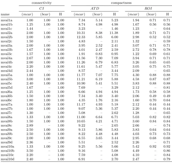
As the results show (see Tables 6 and 7), together with its simplicity, the other advantage of the overlapping constraints here defined is that they also produce good shape solutions in what concerns the compactness and the connectivity.

In these tables, results are grouped for evaluating connectivity (CI) and compactness (AT D and ROI). In each of these groups, columns (mcar ), (bcar ) and H present the corresponding values for models (mcar ) and (bcar ) and for the heuristic, respectively. As usual, the first column refers to the instance name.

It should be remarked that model (nor ), through a MIP solver or the heuristic, assigns tasks to vehicles, and its solutions are used both by (bcar ) and the BCARP heuristic. That is, the minimum objective value computed,

N O, is imposed as an upper bound for the number of shared nodes in (bcar ),

and the tasks assigned to each vehicle in the best (nor ) solution are used by the heuristic to design each vehicle route.

Table 6: Shape measures – mval instances.

connectivity compactness

CI AT D ROI

name (mcar ) (bcar ) H (mcar ) (bcar ) H (mcar ) (bcar ) H

mval1a 1.00 1.00 1.00 7.34 5.14 5.23 1.94 0.71 0.71 mval1b 1.25 1.00 1.00 8.74 4.98 4.98 1.67 0.56 0.56 mval1c 1.44 – 1.00 3.23 – 1.46 1.23 – 0.64 mval2a 2.00 1.00 1.00 10.31 8.38 11.38 1.89 0.71 0.71 mval2b 2.00 1.00 1.00 12.33 5.85 6.00 2.98 0.52 0.52 mval2c 1.50 – 1.00 4.83 – 2.11 1.32 – 0.59 mval3a 2.00 1.00 1.00 3.95 2.52 2.41 3.07 0.71 0.71 mval3b 1.67 1.00 1.00 4.01 2.47 2.59 2.72 0.78 0.78 mval3c 1.57 1.00 1.00 1.91 0.83 0.95 1.22 0.69 0.61 mval4a 2.67 1.00 1.00 11.56 7.30 7.09 3.94 0.71 0.71 mval4b 2.00 1.00 1.00 11.26 6.79 6.83 3.26 0.65 0.65 mval4c 2.20 1.00 1.00 11.61 5.47 5.77 3.05 0.75 0.75 mval4d 2.44 – 1.00 8.57 – 3.44 2.09 – 0.65 mval5a 1.00 1.00 1.00 11.77 7.07 7.75 4.30 0.88 0.88 mval5b 3.00 1.00 1.00 11.21 6.19 5.88 4.58 0.87 0.87 mval5c 2.40 1.00 1.00 10.90 5.41 5.51 3.83 0.88 0.88 mval5d 1.67 – 1.00 7.69 – 3.29 2.12 – 0.81 mval6a 1.25 1.00 1.00 6.66 4.94 4.94 1.73 0.58 0.58 mval6b 1.50 1.00 1.00 7.34 3.40 3.40 2.06 0.49 0.49 mval6c 1.80 1.00 1.00 4.35 1.76 2.16 1.60 0.70 0.64 mval7a 1.00 1.00 1.00 11.17 4.93 5.18 2.12 0.44 0.44 mval7b 1.00 1.00 1.00 9.07 5.36 5.37 2.20 0.44 0.44 mval7c 1.30 – 1.00 5.08 – 2.62 1.28 – 0.65 mval8a 1.33 1.00 1.00 11.00 6.64 6.71 5.03 0.82 0.82 mval8b 1.50 1.00 1.00 10.65 4.21 4.71 3.60 0.84 0.84 mval8c 2.89 – 1.00 9.22 – 2.65 2.66 – 0.74 mval9a 2.50 1.00 1.00 9.13 5.86 5.83 3.83 0.64 0.64 mval9b 2.50 1.00 1.00 8.22 4.48 4.48 4.03 0.73 0.73 mval9c 2.00 1.00 1.00 6.55 3.65 3.44 2.95 0.68 0.68 mval9d 2.36 – 1.00 5.51 – 2.52 2.26 – 0.71 mval10a 1.33 1.00 1.00 9.25 5.56 5.66 5.42 0.92 0.92 mval10b 3.50 – 1.00 9.16 – 5.08 4.49 – 0.86 mval10c 2.20 – 1.00 7.59 – 4.08 4.10 – 0.84 mval10d 2.40 – 1.00 6.91 – 2.70 2.47 – 0.79

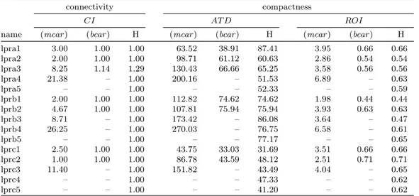
Table 7: Shape measures – lpr instances.

connectivity compactness

CI AT D ROI

name (mcar ) (bcar ) H (mcar ) (bcar ) H (mcar ) (bcar ) H

lpra1 3.00 1.00 1.00 63.52 38.91 87.41 3.95 0.66 0.66 lpra2 2.00 1.00 1.00 98.71 61.12 60.63 2.86 0.54 0.54 lpra3 8.25 1.14 1.29 130.43 66.66 65.25 3.58 0.56 0.56 lpra4 21.38 – 1.00 200.16 – 51.53 6.89 – 0.63 lpra5 – – 1.00 – – 52.33 – – 0.59 lprb1 2.00 1.00 1.00 112.82 74.62 74.62 1.98 0.44 0.44 lprb2 4.67 1.00 1.00 107.81 75.94 75.94 3.93 0.63 0.63 lprb3 8.71 – 1.00 173.42 – 86.08 3.64 – 0.47 lprb4 26.25 – 1.00 270.03 – 76.75 6.58 – 0.61 lprb5 – – 1.00 – – 77.17 – – 0.65 lprc1 2.50 1.00 1.00 43.75 33.03 31.69 3.51 0.66 0.66 lprc2 1.00 1.00 1.00 86.78 43.59 48.12 2.51 0.71 0.71 lprc3 11.40 – 1.00 151.82 – 43.49 4.04 – 0.65 lprc4 – – 1.00 – – 47.33 – – 0.62 lprc5 – – 1.00 – – 41.20 – – 0.62

H: heuristic; –: the MIP solver did not find a feasible solution within the time limit.

Note that a connectivity index value equal to one refers to an optimal solution under this measure, with one connected component per route, as it is observed (see Tables 6 and 7) for the majority of the cases for both the (bcar ) and the heuristic, and contrary to the values achieved by (mcar ). In fact, even for larger lpr instances, when available, this comparison favors the heuristic that produces values equal to 1 (except for lpra3), whereas the corresponding values for (mcar ) are greater than 10.

Again, routes compactness, evaluated through indexes AT D and ROI (Tables 6 and 7), show the advantages of imposing the new constraint.

Although identical values are obtained by (bcar ) and the heuristic for the connectivity and the compactness indexes, it should be emphasized that the second phase of the heuristic always gets a feasible solution within the time limit of one hour.

To sum up, solution objective values given by (bcar ) greater than the ones from (mcar ) are expected, since additional conditions are imposed to the vehicle routes. Nevertheless, these increases in the objective values may be considered acceptable, as they are compensated by “nicer” solution shapes.

7. Conclusions

In this paper we have introduced the BCARP problem, which is defined as the MCARP with an upper bound on the number of common nodes to

different routes.

Quite often the optimal solutions produced by MCARP do not exhibit nice characteristics to be implemented in practice, namely the shape of the routes are not attractive to practitioners.

By defining the concept of overlapped nodes and by imposing a constraint bounding the number of such nodes on the solutions of the original MCARP, our results show that the resulting solutions exhibit much better character-istics according to three “nicety” measures proposed in the paper.

As expected the optimal solutions of the new problem are more costly than the corresponding optimal solutions of the problem without the extra constraint. However, the increase in the cost is acceptable when we compare what we gain by making the routes “nicer”.

We have also developed a heuristic that produces acceptable solutions for the instances that are not easy solved by the proposed MIP model. This method also provides “nice” feasible solutions, with acceptable gap values in small computational times. The heuristic suggested in Section 4.2 for the NOMCARP subproblem allows us to improve the feasible solutions for the BCARP as well as to improve the “nice” characteristics.

Future work will deepen the study on the properties of attractive routes. These will also address the inclusion or exclusion of the depot from the route shaping process.

Acknowledgement This work is supported by National Funding from

FCT-Funda¸c˜ao para a Ciˆencia e a Tecnologia, under the projects PEsT-OE/MAT/ UI0152 and PTDC/EGE-GES/121406/2010. The authors wish to thank the two anonymous referees for their careful reading of the manuscript and their comments and suggestions that have contributed to improve the paper.

Appendix A. Proof of the proposition

Proof. Given a feasible solution (x, y, f, n) of (nomcar ), consider (z, n) with

the same vector n, and z defined by zap_ij = xp_ij for (i, j) ∈ AR and zepij = xp_ij+ xp_ji for{i, j} ∈ ER. We show that (z, n) is feasible for (nor ) and has the

same objective value as the given solution of (nomcar ). Indeed, the objective functions are the same; satisfaction of constraints (5a) and (5b) follows from the definition of z and from (1b) and (1c); satisfaction of constraints (5d) and (5e) also follows from the definition of the variables and from (4a) and (4b); satisfaction of constraints (5f) and (5g) follows from (1b), (1c), and

(1j). To see that capacity constraints (5c) are satisfied, observe that for all p we have ∑ (i,j)∈AR qijzapij + ∑ {i,j}∈ER qijzepij = ∑ (i,j)∈R qijxpij = ∑ (s,j)∈A f_sjp ≤ W ∑ (s,j)∈A yp_sj ≤ W,

where the first equality follows from the definition of the z variables, and the second from constraints (1g). The first inequality follows from (1i), as

{(s, j) ∈ A} ⊆ AD, and the second from (1e).

Conversely, consider a solution (z, n) feasible for (nor ). We build a solu-tion (x, y, f, n) for (nomcar ) with the same n variables. For each p, if zp _{= 0}

let xp _{= 0, y}p _{= 0 and f}p

= 0; otherwise, let xp_ij = zap_ij for (i, j) ∈ AR, and xp_ij = zep_ij, xp_ji = 0 for {i, j} ∈ ER.

To define variables yp_ij and f_ijp, find a route Up _{= (u}

1, u2, . . . , uT) starting

and ending in the depot s, passing through all arcs u = (i, j) such that

xp_ij = 1, without visiting node s except as the start and end of the route. Such a route exists because of the strong connectivity assumption on the subgraph of G spanned by N\ {s}, although it may pass more than once on some arcs. Observe that u1, . . . , uT depend on p, but to make the notation

lighter we omit the superscript p from this and other terms for which that dependence follows from the context.

Let yp_ij be the number of times arc (i, j) is traversed without service in route Up_{, that is, y}p

ij = |{t : ut = (i, j)}| if (i, j) ∈ AD and ypij =|{t : ut =

(i, j)}| − xp_ij if (i, j) ∈ R. f_ijp can be defined as follows. For t = 1, . . . , T , let φut be the total demand in the set of arcs St = {ut, . . . , uT} (without

repetitions) that is satisfied in route p, that is φut =

∑ (i,j)∈St∩R qijxpij. Finally, let f_ijp = ∑ t:ut=(i,j) φut. Observe that f p ij = 0 if (i, j) /∈ Up.

We show that (x, y, f, n) is feasible for (nomcar ). Satisfaction of con-straints (1j), (1k), (1l) and (4c) follows from the definition of the variables; constraints (1b) and (1c) follow from the definition of x and from (5a) and (5b).

To see that constraints (1d) are satisfied, let p∈ {1, . . . , P } and i ∈ N. Hence, from the definition of yp_ij,

∑

j:(i,j)∈A

y_ijp − ∑ j:(j,i)∈A

= ∑ j:(i,j)∈AD |{t : ut = (i, j)}| − ∑ j:(j,i)∈AD |{t : ut = (j, i)}|+ + ∑ j:(i,j)∈R ( |{t : ut= (i, j)}| − x p ij ) − ∑ j:(j,i)∈R ( |{t : ut= (j, i)}| − x p ji ) = = ∑ j:(i,j)∈A |{t : ut= (i, j)}|− ∑ j:(j,i)∈A |{t : ut = (j, i)}|− ∑ j:(i,j)∈R xp_ij+ ∑ j:(j,i)∈R xp_ji= = ∑ j:(j,i)∈R xp_ji− ∑ j:(i,j)∈R xp_ij.

The last equality follows from Up _{being a route, so the two left sums in the}

third expression are equal for all i ∈ N.

Satisfaction of constraints (1e) follows from the fact that route Up leaves

s at most once, through a non-service arc, for each p ∈ {1, . . . , P }. Now from

the definition of f, we have for all p and i∈ N \ {s} ∑

j:(j,i)∈A

f_jip − ∑ j:(i,j)∈A

f_ijp = ∑

t:ut=(j,i)∈A

φut −

∑

t′:ut′=(i,k)∈A

φut′.

Observe that for i ∈ N \ {s} and t ∈ {1, . . . , T − 1}, ut = (j, i)∈ A if and

only if ut+1= (i, k)∈ A, so the above expression equals

∑

t:ut=(j,i)∈A

(φut − φut+1) =

∑

t:ut=(j,i)∈A

  ∑ (k,l)∈St∩R qklxpkl− ∑ (k,l)∈St+1∩R qklxpkl   = = ∑ t:ut=(j,i)∈R qjixpji = ∑ j:(j,i)∈R qjixpji,

where the first equality follows from the definition of φut and the last is

true because route Up _{visits all arcs (k, l)} ∈ R such that xp

kl = 1. Hence,

constraints (1f) are satisfied.

Constraints (1g) follow from the fact that for all p, route Up _{leaves node} s at most once and, when it does it, it uses arc u1 ∈ AD. Therefore

∑ (s,j)∈A f_sjp = f_up₁ = φp_u1 = ∑ (i,j)∈S1∩R qijx p ij = ∑ (i,j)∈R qijx p ij,

because route Up _{visits all arcs u∈ R such that x}p ij = 1.

If f_ijp = 0, constraints (1h) or (1i) are satisfied because xp_ij, yp_ij, W ≥ 0. Suppose f_ijp > 0. Thus, f_ijp = ∑ t:ut=(i,j) φut = ∑ t:ut=(i,j) ∑ (k,l)∈St∩R qklxpkl≤ ∑ t:ut=(i,j) ∑ (k,l)∈R qklxpkl= = ∑ t:ut=(i,j)   ∑ (k,l)∈AR qklza p kl+ ∑ {k,l}∈ER qklze p kl   ≤ W|{t : ut = (i, j)}|,

where the last inequality follows from (5c). The last term is equal to W (yp_ij+

xp_ij) if (i, j) ∈ R, and equal to W y_ijp if (i, j) ∈ AD. Hence constraints (1h)

and (1i) are also satisfied in this case.

Therefore, (x, y, f, n) is feasible for (nomcar ). Since variables n and the objective function are the same in both models, it follows that (x, y, f, n) and (z, n) have the same value. This concludes the proof.

References

Amaya, A., Langevin, A., Tr´epanier, M., 2007. The capacitated arc routing problem with refill points. Operations Research Letters 35 (1), 45–53.

Assis, L. S., Franca, P. M., Usberti, F. L., 2014. A redistricting problem applied to meter reading in power distribution networks. Computers & Operations Research 41, 65–75. Bautista, J., Fern´andez, E., Pereira, J., 2008. Solving an urban waste collection problem

using ants heuristics. Computers & Operations Research 35 (9), 3020–3033.

Belenguer, J. M., Benavent, E., Lacomme, P., Prins, C., 2006. Lower and upper bounds for the mixed capacitated arc routing problem. Computers & Operations Research 33 (12), 3363–3383.

Benavent, E., Corber´an, A., Gouveia, L., Mour˜ao, M., Pinto, L., 2014. Profitable mixed capacitated arc routing and related problems. TOP doi: 10.1007/s11750-014-0336-x. Bozkaya, B., Erkut, E., Laporte, G., 2003. A tabu search heuristic and adaptive memory

procedure for political districting. European Journal of Operational Research 144 (1), 12–26.

Cattrysse, D., Van Oudheusden, D., Lotan, T., 1997. The problem of efficient districting. OR Insight 10 (4), 9–13.

Corber´an, A., Prins, C., 2010. Recent results on arc routing problems: An annotated bibliography. Networks 56 (1), 50–69.

Dror, M. (Ed.), 2000. Arc Routing: Theory, Solutions and Applications. Kluwer Academic Publishers, Dordrecht.

Ghiani, G., Guerriero, F., Improta, G., Musmanno, R., 2005. Waste collection in Southern Italy: solution of a real-life arc routing problem. International Transactions in Opera-tional Research 12 (2), 135–144.

Ghiani, G., Lagan`a, D., Manni, E., Musmanno, R., Vigo, D., 2014. Operations research in solid waste management: A survey of strategic and tacticaal issues. Computers and Operations Research 44, 22–32.

Golden, B. L., Wong, R. T., 1981. Capacitated arc routing problems. Networks 11 (3), 305–315.

Gonzalez-Ram´ırez, R. G., Smith, N. R., Askin, R. G., Miranda, P. A., S´anchez, J. M., 2011. A hybrid metaheuristic approach to optimize the districting design of a parcel company. Journal of Applied Research and Technology 9 (1), 19–35.

Gouveia, L., Mour˜ao, M. C., Pinto, L. S., 2010. Lower bounds for the mixed capacitated arc routing problem. Computers & Operations Research 37 (4), 692–699.

Jarrah, A. I., Bard, J. F., 2012. Large-scale pickup and delivery work area design. Com-puters & Operations Research 39 (12), 3102–3118.

Kim, B. I., Kim, S., Sahoo, S., 2006. Waste collection vehicle routing problem with time windows. Computers & Operations Research 33 (12), 3624–3642.

Lei, H., Laporte, G., Guo, B., 2012. Districting for routing with stochastic customers. EURO Journal on Transportation and Logistics 1 (1–2), 67–85.

Lin, H. Y., Kao, J. J., 2008. Subregion districting analysis for municipal solid waste collection privatization. Journal of the Air & Waste Management Association 58, 104– 111.

Lu, Q., Dessouky, M., 2006. A new insertion-based construction heuristic for solving the pickup and delivery problem with time windows. European Journal of Operatonal Re-search 175, 672–687.

MacEachren, A. M., 1985. Compactness of geographic shape: Comparison and evaluation of measures. Geografiska Annaler. Series B, Human Geography 67 (1), 53–67.

Matis, P., 2008. Decision support system for solving the street routing problem. Transport 23 (3), 230–235.

Mour˜ao, M. C., Amado, L., 2005. Heuristic method for a mixed capacitated arc routing problem: A refuse collection application. European Journal of Operational Research 160 (1), 139–153.

Mour˜ao, M. C., Nunes, A. C., Prins, C., 2009. Heuristic methods for the sectoring arc routing problem. European Journal of Operational Research 196 (3), 856–868.

Mourgaya, M., Vanderbeck, F., 2007. Column generation based heuristic for tactical plan-ning in multi-period vehicle routing. European Journal of Operational Research 183 (3), 1028–1041.

Muyldermans, L., Cattrysse, D., Van Oudheusden, D., 2003. District design for arc-routing applications. Journal of the Operational Research Society 54 (11), 1209–1221.

Muyldermans, L., Cattrysse, D., Van Oudheusden, D., Lotan, T., 2002. Districting for salt spreading operations. European Journal of Operational Research 139 (3), 521–532. Perrier, N., Langevin, A., Campbell, J. F., 2008. The sector design and assignment problem for snow disposal operations. European Journal of Operational Research 189 (2), 508– 525.

Poot, A., Kant, G., Wagelmans, A., 2002. A savings based method for real-life vehicle routing problems. Journal of the Operations Research Society 53, 57–68.

Ramos, T. R. P., Oliveira, R. C., 2011. Delimitation of service areas in reverse logistics networks with multiple depots. Journal of the Operational Research Society 62 (7),

1198–1210.

R´ıos-Mercado, R. Z., Fern´andez, E., 2009. A reactive GRASP for a commercial terri-tory design problem with multiple balancing requirements. Computers & Operations Research 36 (3), 755–776.

Salazar-Aguilar, M. A., R´ıos-Mercado, R. Z., Gonz´alez-Velarde, J. L., Molina, J., 2012. Multiobjective scatter search for a commercial territory design problem. Annals of Op-erations Research 199 (1), 343–360.

Tang, H., Miller-Hooks, E., 2006. Interactive heuristic for practical vehicle routing problem with solution shape contraints. Journal of the Transportation Research Board 1964, 9– 18.

Teixeira, J., Antunes, A. P., Sousa, J. P., 2004. Recyclable waste collection planning – a case study. European Journal of Operational Research 158 (3), 543–554.

Wøhlk, S., 2008. A decade of capacitated arc routing. In: Golden, B., Raghavan, S., Wasil, E. (Eds.), The Vehicle Routing Problem: Latest Advances and New Challenges. Operations Research/Computer Science Interfaces. Springer, Berlin, pp. 29–48.