Nonlinear dynamics within macroeconomic factors and stock market in Portugal 1993-2003

NONLINEAR DYNAMICS WITHIN MACROECONOMIC FACTORS AND STOCK MARKET IN PORTUGAL, 1993-2003

DIONISIO, Andreia * MENEZES, Rui ** MENDES, Diana VIDIGAL DA SILVA, Jacinto

Abstract

The main objective of this paper is to assess how mutual information as a measure of global dependence between stock markets and macroeconomic factors can overcome some of the weaknesses of the traditional linear approaches commonly used in this context. One of the advantages of mutual information is that it does not require any prior assumption regarding the specification of a theoretical probability distribution or the specification of the dependence model. This study focuses on the Portuguese stock market where we evaluate the relevance of the macroeconomic and financial variables as determinants of the stock prices behaviour.

JEL Classification: C14, C22, C32

Keywords: Nonlinear dependence, mutual information, macroeconomic and financial factors

1. Introduction

It is quite common to find in the financial literature theories and models based on the efficient market hypothesis, which implies that prediction and forecasting based on historical rates of return or other factors are not possible to perform in practice. This argument has been reinforced by empirical findings that stock prices follow a random walk process. Therefore, an alternative way to study the relationship between the economic activity represented by macroeconomic factors and the behaviour of prices in the stock market lies on the analysis of long-run trends based on monthly observations [Pesaran et al. (1995)].

Traditionally, the study of such links has been made on the basis of linear models. However, there are many authors that argue that this type of analysis is in general inconclusive because linear independence is not synonymous of independence, being thus necessary to ascertain the possibility of the existence of nonlinear dependence [Darbellay (1998); Maasoumi et al. (2002)].

This paper investigates the relationship between the behaviour of certain economic factors and the Portuguese stock market prices by means of linear and nonlinear approaches based upon traditional single equation linear models and global dependence tests (linear and nonlinear) using mutual information and the global correlation coefficient. The main goal is to access dependence in a global way, linear and nonlinear, and independently of any previously assumed model. In this context we use in this paper

* Andreia Dionisio & Jacinto Vidigal da Silva: University of Evora, Center of Business Studies CEGAGE-UE, Department of Management, Largo dos Colegiais, 2, 7000 Evora, Portugal (correspondent author: andreia@uevora.pt);

** Rui Menezes & Diana Mendes: ISCTE, Department of Quantitative Methods, Av. ForcasArmadas, 1649-025 Lisboa, Portugal

mutual information as an attempt to evaluate the ability of this measure to capture dependence in financial time series.

The rest of the paper is organized as follows. Section 2 presents the theoretical framework for accessing the relationship between the behaviour of stock markets and various macroeconomic and financial factors. Section 3 presents mutual information as a measure of global dependence, describes the properties of mutual information and the estimation procedure adopted. In Section 4 we describe and justify the data used in our analysis and the results obtained from implementing the methodologies adopted in our study. Both single linear equation models and nonlinear mutual information models were employed in our context as referred to above. The final Section presents some concluding remarks of this study.

2. Background

Asset prices are commonly believed to react sensitively to economic news. Furthermore, daily experience seems to support the view that individual asset prices are influenced by a wide variety of unanticipated events and that some events have more persuasive effects on asset prices than others. In this context, the portfolio theory, based on the diversification effect, focused its attention on the systematic risk.

There are several empirical studies based on linear models, that highlight the importance of some macroeconomic variables [Chen et al. (1986); Pesaran et al. (1995); Haugen et al. (1996)], business conditions [Fama et al. (1989); Fama (1990); Fama et al. (1993)] and the real activity [McQueen et al. (1993)], on the behaviour of the stock market returns. In this context, there are alternative approaches that consider the existence of bidirectional relationships between stock returns and macroeconomic variables, revealing in some cases that it is the stock market that "leads" the real economic activity [see e.g. Fama (1990); Binswanger (2001)].

Most of the models used to study the relationship between the behaviour of stock returns and macroeconomic and financial variables were based on linear regression techniques estimated by OLS. In this sense, the possible nonlinear effect was omitted as well as the possible feedback effects. Besides, the estimated coefficients may suffer severe biases since the residuals hardly behave as white noise. Thus, the use of nonlinear models to explain in a different way the relationship between macroeconomic variables and stock returns may bring some "fresh air" into this field [e.g. Stuzer (1995); Qi (1999); Maasoumi et al. (2002)]

Globally, we retain an overall impression that there is a set of variables that may affect stock returns and can show some feedback effects. The majority of the studies in this field point to the existence of predictability of stock returns, but the rejection of the efficient market hypothesis based on this evidence was not sufficient for the majority of the referred authors.

2.1. The nonlinear approach - mutual information: One of the most practical ways to

evaluate the (in)dependence between two vectors of random variables X,Y is to consider a measure that assumes the value 0 when there is total independence and 1 when there is total dependence. Let p_X,Y

(

A B×

)

be the joint probability distribution of

(

X, Y

)

and

( )

the observation space of X and B is a subset of the observation space of Y, such that we

can evaluate the expression: ( )

( ) ( ) ln p A B p A p B × X,Y X Y

. If the two events are independent, then

(

)

( ) ( )

p_X,Y A B× = p_X A p_Y B , and so this equation will take the value zero.

Granger, Maasoumi and Racine (2004) consider that a good measure of dependence should satisfy the following six "ideal" properties:

(a) It must be well defined for both continuous and discrete random variables;

(b) It must be normalized to zero if the random variables (or vectors of random variables) are independent, and lying between -1 and +1, in general;

(c) The absolute value of the measure should be equal to 1 if there is an exact nonlinear relationship between the random variables;

(d) It must be similar or related in a simple way with the linear correlation coefficient in the case of a bivariate normal distribution;

(e) It must be metric in the sense that it is a true measure of "distance" and not just a measure of "divergence";

(f) It must be an invariant measure under continuous and strictly increasing transformations.

2.2 Mutual information properties: The concept of mutual information comes originally

from the theory of communication and measures the information of a random variable contained in another random variable. The definition of mutual information goes back to Shannon (1948) and the theory was extended and generalized by Gelfand, Kolmogorov and Yaglom (1956) [in Darbellay (1998)]. According to Pompe (1998), the concept of mutual information is very useful to analyze statistical dependences in scalar or multivariate time series as well as for detecting fundamental periods, detecting optimal time combs for forecasting and for modelling and analyzing the (non)stationarity of data. Some of those potentialities have been explored by Granger and Lin (1994) and Darbellay and Wuertz (2000), whose results reveal that mutual information varies in a nonstationary time series framework.

The properties of mutual information appear to confirm its importance as a measure of dependence [Soofi (1997); Darbellay et al. (1999), (2000); Darbellay (1998, 1999); Bernhard et al. (1999)]. Some of those properties will be presented and explored in this Subsection.

If

p

X

,

p

Yand

p

X Y, denote the pdf of the random variables X, Y and (X,Y),

respectively, then the mutual information is given by1_:

(

)

( )

_{( ) ( )}

,

( )

, , , , log X Y X Y X Y p x y I X Y p x y dxdy p x p y =

∫∫

(1)

Mutual information is a nonnegative measure [Kullback, (1968)], being equal to zero if and only if X and Y are statistically independent. In this way, the mutual information between two random variables X and Y can be regarded as a measure of dependence

1 _{The selection of the base of the logarithm is irrelevant, but is convenient to distinguish among} results: log - entropy measure in bits; log - entropy measure in dits; ln - entropy measure in nats.

between these variables, or even better, it can be regarded as a measure of the statistical correlation between X and Y. However, we can not say that X is causing Y or vice-versa.

The statistic given in equation (1) satisfies some of the properties mentioned above, namely property (a) and after some transformations, will also satisfy properties (b), (c) and (d) [Granger et al. (2004)].2

In order to satisfy the properties (b) and (d) we need to define a measure that can be directly comparable with the linear correlation coefficient. In equation (1), we have 0≤I(X,Y)≤+∞, which hampers eventual comparisons between different samples. However, we can easily compare the mutual information with the covariance, since both vary between 0 and +∞.

To obtain a statistic that satisfies property (d) without losing the properties (a) to (c) we can define an equation similar to that displayed in (2). In this context Granger and Lin (1994), Darbellay (1998) and Soofi (1997), among others, have used a standard measure for the mutual information, referred to as the global correlation coefficient, defined by:

(

)

₁ 2I( )

e

λ _{X, Y = −} − X,Y ₍₂₎

This measure varies between 0 and 1 being thus directly comparable with the linear correlation coefficient.

The function λ(X,Y) captures the overall linear and nonlinear dependence between X

and Y. This measure can be regarded as a measure of predictability based on an empirical

probability distribution, although it does not depend on any particular model of predictability. In this particular case, the above mentioned properties assume the following form: (i) λ(X,Y)=0, if and only if X contains no information on Y; (ii) λ(X,Y)=1, if exists a perfect relationship between the vectors X and Y. This is the farthest

case of determinism; (iii) when modelling the input-output pair (X,Y) by any model with input X and output U= f

( )

X , where f is a function of X, the predictability of Y by U

cannot exceed the predictability of Y by X, i.e., λ(X,Y)≥λ(U,Y).

It is well known that the Gaussian distribution maximizes Shannon entropy for the first and second moments. This implies that the Shannon entropy of any distribution is bounded upwards by the normal mutual information (NMI), and depends on the covariance matrix [Kraskov et al. (2003)]. Let us consider a normal probability distribution, defined in an Euclidian space with dimension d. Then the normal mutual information for (X,Y) is given by:

(

)

1logdet det

(

2 det V V I V = X Y = X, Y NMI X, Y

)

Y (3)

where V is the covariance matrix of (X,Y) and

det

are respectively the covariance matrices of X and Y and det represents the determinant. It can be shown that

the argument of the logarithm on the right-hand side of (3) depends only on the matching coefficients of linear correlation [see e.g. Darbellay (1998)]. Thus, for example, if d=2, that is, for (X,Y)=(X,Y) equation (4) takes the form [Kullback (1968)]:

,det

V

_X

V

(

_,

)

1_{log 1}

(

2

(

_,

)

2 NMI X Y = − −r X Y

)

.

(4)

2 _{The demonstration of some theorems about mutual information properties can be found in} Kullback, S. (1968). Information Theory and Statistics, Dover, New York.

If the empirical distribution is a normal one, the mutual information can be calculated using (4), because the normal distribution is a "linear" distribution, in the sense that the linear correlation coefficient captures the overall dependence. In this case, any empirical mutual information must be greater than or equal to the normal mutual information [Kraskov et al. (2003)].

Intuitively, one would like to have a measure of predictability that is larger than the measure of linear predictability, i.e.λ≥ . Unfortunately however, this is not always true r

[Darbellay (1998)].3

It is important to note that the difference

(

λ−r

)

does not necessarily captures the

nonlinear part of the dependence. Nevertheless, if the distribution is normal, we do have

(

)

r

(

)

λ X, Y = X, Y , and in R² we have λ

(

X,Y

)

= r X,Y

(

)

[Granger et al. (1994);

Darbellay (1998)].

Another important property of the mutual information is additivity. Basically, this property says that the mutual information can be decomposed into hierarchical levels [Shannon (1948); Kraskov et al. (2003)], that is I

(

X, Y, Z

)

=I

(

(

X, Y Z

)

,

)

+I

(

X, Y

)

.

)

. It follows that I X, Y, Z

(

will be always greater than or equal to I X, Y . By the same

(

)

token, the coefficient of linear determination and the coefficient of linear correlation cannot decrease when one adds more variables to the model.

2.3. The test of independence: On the basis of the properties of mutual information, and

because "independence" is one of the most valuables concepts in empirical econometrics, we can construct a test of independence based on the following hypothesis:H₀:p_{X Y,}

(

x y,

)

= p_X

( ) ( )

x p_Y y ;H₁:p_{X Y,}

(

x y,

)

≠ p_X

( ) ( )

x p_Y y .

H

₀

0

If holds, then and we conclude in favour of the independence between the variables. If holds, then

(

,

)

I X Y =

1

H

I X Y

(

,

)

> 0 and we reject the null hypothesis of independence. The

above hypothesis can be reformulated as follows:

(

)

(

)

0 : , 0; 1: ,

H I X Y = H I X Y > 0.

t

In order to test adequately for the independence between random variables (or vectors of random variables) we need to compute the critical values of the distribution. There are basically three approaches to obtain critical values for our test under the null: (1) asymptotic approximations to the null distribution; (2) simulated critical values for the null distribution and (3) permutation-based critical values for the null distribution.

The critical values for mutual information computed in this paper are based upon simulated critical values for the null distribution of the percentile approach (see Appendix A). These critical values have been found by simulation based upon a white noise, for a number of sample sizes. Given that the distribution of mutual information is skewed, we can adopt a percentile approach to obtain the critical values.

Appendix A lists the 90th_{, 95}th _{and 99}th _{percentiles of the empirical distribution of the}

mutual information for the process y_t =ε with ε_t i i d N. . .

( )

0,1 , having been made

3 _{A situation that can induce λ<r is the small size of the sample. A small size, in this context, is a} sample with n≤500.

5000 simulations for each critical value. This methodology was formerly proposed and applied by Granger, Maasoumi and Racine (2004), and according to these authors, the critical values thus obtained can be used to test for time series serial independence.

One of the difficulties for estimating mutual information on the basis of empirical data lies on the fact that the underlying pdf is unknown. To overcome this problem, there are essentially three different methods to estimate mutual information: (i) histogram-based estimators; (ii) kernel-histogram-based estimators; (iii) parametric methods. In order to minimize the bias that may occur, we will use the marginal equiquantization estimation process (the partition of the space in equiprobable cells), that was proposed by Darbellay (1998, 1999).4

3. Data and results.

The purpose of this study is to evaluate the behaviour of the Portuguese stock market in relation to changes in a set of economic and financial firm factors selected according to the relevant literature in this field [see e.g. Chen et al. (1986), Asprem (1989), Campbell

et al. (1989), Campbell (1991), Hordrick (1992), Fama et al. (1993), McQueen et al.

(1993), Pesaran et al. (1995), Raj et al. (1995), Maasoumi et al. (2002)]. The definition and source of the indicators that were selected, as well as the definition of the variables computed on the basis of the selected indicators, are shown in Table 1.

Table 1. Glossary and definition of indicators.

Indicator Symbol Source and definition

Price index of the Portuguese stock

market t

PI Monthly price index, Source: Data base Datastream

Short-term interest rest

3 _t

Lisbor M

Source: Data base Dhatis Long-term interest

rate Swap10t Source: Data base Dhatis

Dividend yield DYt Dividends/price ratio, Source: Data base Datastream Earnings price ratio EPRt Earnings/price ratio, Source: Data base Datastream Consumer price index IPC_t Source: Data base Datastream

Industrial production

index IPIt Source: INE

Unemployment TD_t Source: Data base Datastream

Oil prices OILt Spot oil prices in the USA market, Source:

http://www.eia.doe.gov/oil_gas/petroleum/info_glance/pric es.html

All the indicators are measured monthly and the period under analysis is October 1993 to October 2003. All the indicators have a unit root according to the Augmented Dickey-Fuller test, so their first differences are stationary variables.

4 _{For a good explanation of this method of estimation see Darbellay, G. (1998) and Darbellay, G.} and Vadja, I. (1999).

All the indicators are measured monthly and the period under analysis is from October 1993 to October 2003. The statistical analysis performed on those indicators revealed that the indicators have a unit root according to the Augmented Dickey-Fuller test and the Elliot-Rothenberg-Stock Point-Optimal test and their first differences are stationary variables.

Since all the indicators are non-stationary, we compute the differences of the logarithms and obtain the respective growth rates. Let ER represent the monthly excess _t

return; the short-term interest growth rate; the long-term interest growth rate; 3 _t Lisbor M ∆ ∆Swap10_t t DY

∆ the dividend yield growth rate; ∆EPR_t the earnings price ratio growth

rate; the growth rate; the monthly industrial production growth rate; the year-on-year industrial production growth rate; the unemployment growth rate and the oil price growth rate.

t IPC ∆ IPC ∆PIM_t t PIA ∆ ∆TD_t t OIL ∆

According to some authors [e.g. Chen et al. (1986), Fama (1990), McQueen et al. (1993)], we should use the unanticipated changes in the variables or the respective innovations. Because some of the time series have evidence of significant autocorrelation and seasonality, it was necessary to filter the series, as shown in Table 2. The filtering process for each new variable was selected according to the Scharwz information criterion and the Akaike information criterion. We performed the Ljung-Box test and in the results there is no evidence of any sign of autocorrelation in all new variables.

Table 2. Filtered series representing the unanticipated changes in the variables.

New variable Process

inovLisbor ARMA( )1, 0 of ∆Lisbor M3

inovSwap ARMA( )1, 0 of ∆Swap10

inovIPC ARMA( )3, 1 of ∆IPCSA, ∆IPCSA is the seasonal effect adjustment of IPC∆

inovPIM ARMA( )2, 0 of ∆IPMSA, ∆IPMSA is the seasonal effect adjustment of ∆PIM

inovPIA ARMA( )1,1 of ∆PIA

inovTD ARMA( )1, 1 of ∆TD

The seasonal adjustment was made through a moving average process. The filtering process was selected according to the SIC and AIC.

We have first computed linear dynamic models to evaluate the relationship between the rate of returns and the macroeconomic and financial variables. The results obtained allow us to identify the following significant explanatory variables for

2 3 2 . : , , , , , , and t t t t t t t t

ER inovSwap DY EPR inovIPC inovPIM inovTD inovTD

OIL

− ∆ ∆ − −

∆

3 t−

Having analyzed the single equation relationship between the macroeconomic and financial variables and the excess return, it is now important to assess the overall performance of the relationship in order to verify whether the set of regressors keep its explanatory power when taken together as a whole. To this end we estimated a multivariate linear dynamic regression model (equation (5)) by OLS and the results are shown in Table 4.

1 2 2 3 4 1 5

6 2 7 8 3 9

,

t t t t t

t t t t t

ER inovSwap DY EPR EPR inovIPC

inovPIM inovTD inovTD OIL

α β β β β β β β β β ε 3 t − − − − = + + ∆ + ∆ + ∆ + + + + + ∆ + − ₍₅₎

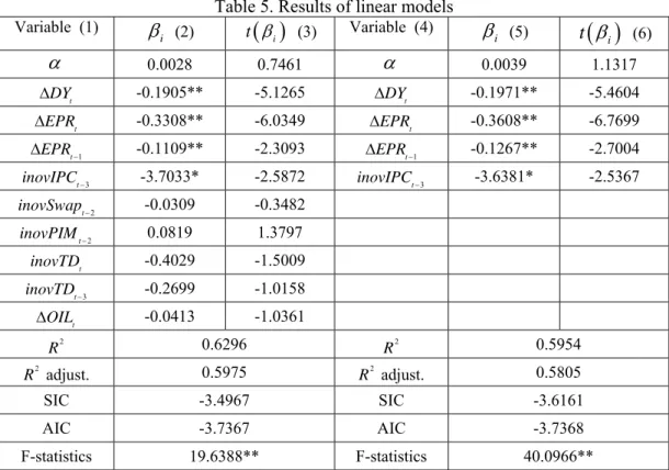
Table 5. Results of linear models Variable (1) i

β

(2) t

( )

β_i (3) Variable (4)

β

_i (5) t

( )

β

_i (6)

α

0.0028 0.7461

α

0.0039 1.1317 t DY ∆ -0.1905** -5.1265 ∆DY_t -0.1971** -5.4604 t EPR ∆ -0.3308** -6.0349 ∆EPR_t -0.3608** -6.7699 1 t EPR₋ ∆ -0.1109** -2.3093 ∆EPR_t−1 -0.1267** -2.7004 3 t inovIPC₋ -3.7033* -2.5872 inovIPC_t−3 -3.6381* -2.5367 2 t inovSwap₋ -0.0309 -0.3482 2 t inovPIM₋ 0.0819 1.3797 t inovTD -0.4029 -1.5009 3 t inovTD₋ -0.2699 -1.0158 t OIL ∆ -0.0413 -1.0361 2 R 0.6296 R2 0.5954 2 adjust. R 0.5975 R2 adjust. 0.5805 SIC -3.4967 SIC -3.6161 AIC -3.7367 AIC -3.7368 F-statistics 19.6388** F-statistics 40.0966**

Notes. Results of linear models described in equation (5) in columns (1), (2) and (3). Columns (4), (5) and (6) refer to the linear regression model, where the independent variables are those that exhibit statistical significance in the global model. We made several statistical tests on the residual of those models, namely the LM test, the ARCH LM test, the Jarque-Bera test and the stability tests CUSUM and CUSUM-Q. The results only allow the rejection of the null hypothesis of the Jarque-Bera tests, so the residuals are not normally distributed. ** refers to 1% significant level and * refers to 5% significant level.

The results displayed in Table 4 show that the only significant explanatory variables that are retained in the multivariate model are: ∆DY_t,∆EPR_t,∆EPR_t−1 and inovIPC_t−3. Not surprisingly, however, we should note that there are precisely the financial variables

that appear to maintain some explanatory and predictive power on the excess return. In what refers to the macroeconomic variables, only the

presents statistical significance in a multivariate context, showing a negative correlation with the excess return. These results are in line with the results reported by other authors, namely inter alia Fama (1990), Fama and French (1993), and Maasoumi and Racine (2002).

(

∆DYt,∆EPRt,∆EPRt−1

)

3 t inovIPC₋

The results reported above help us to identify the extent of the linear dependence that exists in the empirical data used in our analysis. However, it does say very little about the

amount of nonlinear dependence that may also occurs in data. Furthermore, if we only consider the linear relationships or dependencies, we are simultaneously assuming that these relationships are time invariant, which is not usually consistent with the empirical evidence.

In this research work we use mutual information and the global correlation coefficient as measures of global dependence, where this statistic can be compared with the usual measure of linear correlation.

We have computed the mutual information (I), the normal mutual information (NMI), the global correlation coefficient (λ) and the linear correlation coefficient (r) between the excess return in levels and each of the remaining variables measured in levels and with lags (see Tables 5 and 6). We should emphasize that mutual information takes into account the bidirectional relationships that can be established between the variables.

According to the results presented in Tables 5 and 6 we can see that the empirical mutual information (I) is higher in most cases than the normal mutual information (NMI), as well as the global correlation coefficient (λ) is higher than the linear correlation coefficient (r). These differences appear to reveal the presence of nonlinear dependence for the majority of the pairs of variables under study. The relationships that show statistical significance are evidenced in the Tables 5 and 6. The small number of statistically significant global dependence coefficients between the variables may be caused by the small sample sizes (about 118 observations) obtained, which may underestimate the value of the mutual information.

Table 5. Mutual information (I) in nats, global correlation coefficient (λ), normal mutual information (NMI) and linear correlation coefficient (r) between ERt and each of the

individual variables for different lags

I λ NMI r inovLisbor t 0.0413* 0.2816 0.0083 0.1285 inovLisbor t-1 0.0175 0.1855 0.0128 0.1591 inovLisbor t-2 0.0083 0.1283 0.0060 0.1091 inovLisbor t-3 0.0024 0.0692 0.0011 0.0464 inovSwap t 0.0043 0.0925 0.0009 0.0412 inovSwap t-1 0.0036 0.0847 0.0030 0.0775 inovSwap t-2 0.0195 0.1956 0.0170 0.1830 inovSwap t-3 0.0095 0.1372 0.0009 0.0412 ∆DY t 0.7740** 0.8873 0.2182** 0.5946 ∆DY t-1 0.0103 0.1428 0.0065 0.1136 ∆DY t-2 0.0001 0.0167 0.0006 0.0346 ∆DY t-3 0.0018 0.0599 0.0115 0.1510 ∆EPR t 0.7108** 0.8710 0.2973** 0.6695 ∆EPR t-1 0.0599* 0.3360 0.0193 0.1944 ∆EPR t-2 0.0001 0.0141 0.0001 0.0100 ∆EPR t-3 0.0083 0.1283 0.0071 0.1187 inovIPC t 0.0010 0.0436 0.0165 0.1800 inovIPC t-1 0.0009 0.0424 0.0001 0.0141 inovIPC t-2 0.0009 0.0424 0.0009 0.0424 inovIPC t-3 0.0262 0.2259 0.0198 0.1970

Table 6. Mutual information (I) in nats, global correlation coefficient (λ), normal mutual information (NMI) and linear correlation coefficient (R) between ERt and each of the individual

variables for different lags

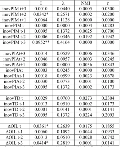
I λ NMI r inovPIM t+3 0.0010 0.0440 0.0005 0.0300 inovPIM t+2 0.0342* 0.2571 0.0002 0.0200 inovPIM t+1 0.0064 0.1128 0.0000 0.0000 inovPIM t 0.0000 0.0000 0.0004 0.0283 inovPIM t-1 0.0095 0.1372 0.0025 0.0700 inovPIM t-2 0.0006 0.0346 0.0192 0.1942 inovPIM t-3 0.0952** 0.4164 0.0000 0.0000 inovPIAt+3 0.0014 0.0529 0.0006 0.0346 inovPIAt+2 0.0046 0.0957 0.0003 0.0245 inovPIAt+1 0.0000 0.0000 0.0036 0.0843 inovPIAt 0.0003 0.0245 0.0000 0.0000 inovPIAt-1 0.0018 0.0599 0.0023 0.0678 inovPIAt-2 0.0030 0.0773 0.0001 0.0100 inovPIAt-3 0.0095 0.1372 0.0002 0.0173 inovTD t 0.0029 0.0760 0.0273 0.2304 inovTD t-1 0.0013 0.0510 0.0002 0.0173 inovTD t-2 0.0001 0.0141 0.0001 0.0141 inovTD t-3 0.0095 0.1372 0.0224 0.2093 ∆OIL t 0.0361* 0.2639 0.0175 0.1855 ∆OIL t-1 0.0060 0.1092 0.0044 0.0933 ∆OIL t-2 0.0013 0.0510 0.0028 0.0742 ∆OIL t-3 0.0414* 0.2819 0.0001 0.0141

** refers to 1% significant level and * refers to 5% significant level.

The pairs of variables

(

ER_t,∆DY_t

)

;

(

ER_t,∆EPR_t

)

and

(

ER_t,∆EPR_t−1

)

, present the

highest level of global dependence, which can be an indicator of the presence of nonlinear dependence. The large differences between λ and r in these cases (and between I and

NMI) may be caused by the fact that the variables are not normally distributed and the

residuals resulting from estimating the linear regression models previously calculated show evidence of autocorrelation and heteroscedasticity. In this context, the simple linear regression analysis may not be sufficient to analyze the level of dependence between the excess return and the macroeconomic and financial variables.

If we take into account all the variables that show statistical significance in this preliminary study and calculate the mutual information between them, we obtain the following result: 1 2 3 3 , , , , 1.8517 , , , t t t t t t t t t

ER inovLisbor DY EPR EPR I

inovPIM inovPIM oil oil

− + − − ∆ ∆ ∆ = ∆ ∆ ⎛ ⎞ ⎜ ⎟ ⎝ ⎠ (6)

which means that λ=0.9876. However, the value of the mutual information of equation (6) is not statistically significant. This fact could be a sign that we should eliminate some variables without great impact on the value of mutual information, in order to increase the degrees of freedom.

To this end, we drop each variable individually and in turn, except ER , in order to _t

obtain the new values of mutual information. We computed the following models:

1 2 3 , , , , 1.4154 * , , t t t t t t t t

ER inovLisbor DY EPR EPR

I

inovPIM inovPIM OIL

− + − ∆ ∆ ∆ = ∆

⎛

⎞

⎜

⎟

⎝

⎠

(7) 1 2 3 3 , , , , 1.5455** , , t t t t t t t t

ER inovLisbor DY EPR EPR

I

inovPIM inovPIM OIL

− + − − ∆ ∆ ∆ = ∆

⎛

⎞

⎜

⎟

⎝

⎠

(8) 1 2 3 , , , , 1.3926 , , t t t t t t t t

ER inovLisbor DY EPR EPR

I

inovPIM OIL OIL

− + − ∆ ∆ ∆ = ∆ ∆

⎛

⎞

⎜

⎟

⎝

⎠

(9) 1 3 3 , , , , 1.5134 ** , , t t t t t t t t

ER inovLisbor DY EPR EPR

I

inovPIM OIL OIL

− − − ∆ ∆ ∆ = ∆ ∆

⎛

⎞

⎜

⎟

⎝

⎠

(10) 2 3 3 , , , , 1.4350 * ,

,

, t t t t t t t t ER inovLisbor DY EPR I

inovPIM₊ inovPIM₋ OIL OIL₋

∆ ∆ = ∆ ∆

⎛

⎞

⎜

⎟

⎝

⎠

(11) 1 2 3 3 , , , , 1.2305 ,

,

, t t t t t t t t ER inovLisbor DY EPR I

inovPIM inovPIM OIL OIL

− + − − ∆ ∆ = ∆ ∆

⎛

⎞

⎜

⎟

⎝

⎠

(12) 1 2 3 3 , , , 1.3664 ,

,

, t t t t t t t t

ER inovLisbor EPR EPR

I

inovPIM inovPIM OIL OIL

− + − − ∆ ∆ = ∆ ∆

⎛

⎞

⎜

⎟

⎝

⎠

(13) 1 2 3 3 , , , 1.4117 * ,

,

, t t t t t t t t ER DY EPR EPR I

inovPIM inovPIM OIL OIL

− + − − ∆ ∆ ∆ = ∆ ∆

⎛

⎞

⎜

⎟

⎝

⎠

(14)

The values of mutual information computed in equations (7) to (14) show that when we take away (individually) the variables ∆OIL_t−3,∆OIL_t, inovPIM_t+2, ∆EPR_t−1 or

, the mutual information becomes statistically significant. This result may indicate that the information contribution of those variables (which can be interpreted as a sort of marginal mutual information) is not very strong when analyzed jointly with other variables. We should also note that the variables

t

inovLisbor

3 ,

and

t t t DY EPR inovPIM₋ ∆ ∆ , which

were statistically significant at 1% in the previous analysis (see Tables 5 and 6), are precisely the variables that show here more informative contribution in a set of variables including ER . If we only consider the variables _t ER_t

,

∆DY_t,∆EPR_t

and

inovPIM_t−3, the

value of the mutual information becomes:

(

t, t, t, t 3

)

1.3021*

I ER ∆DY ∆EPR inovPIM₋ = * (15)

which is statistically significant and confirms the existence of linear and possibly nonlinear dependence between these variables.

From the present analysis we can noticed that the set of macroeconomic and financial variables that are more correlated with the excess return is not very different from that found using a linear regression analysis. If we apply the same methodology to the variables used in equation (15) (these variables are statistically significant at 1% in the analysis of global dependence displayed in Tables 5 and 6), the mutual information will assume the value presented in equation (16):

(

t, t, t 3

)

0.4311**

I ∆DY ∆EPR inovPIM₋ = (16)

thus, the mutual information between ER and the set of explanatory variables described _t

in equation (16) is:

(

)

[

t, t, t, t 3

]

0.8710 **

I ER ∆DY ∆EPR inovPIM₋ = (17)

The global dependence between ER and a vector composed by the variables _t 3

,

and

t t t

DY EPR inovPIM₋

∆ ∆ has a value of 0.8710 nats, which corresponds to a global

correlation coefficient of λ=0.9082. If we estimate a linear regression model with these variables, namely:

1 2 3 3

t t

ER = + ∆α β DY+ ∆β EPR +β inovPIM_t− + (18) ε_t

we obtain a linear correlation coefficient of r =0.7420, smaller than the corresponding global correlation coefficient. This difference could be generated by the possible presence of nonlinear dependences, which may be a reflex of the leptocurtosis (fat-tails) and skewness of the residuals resulting from the estimation of equation (18). According to some authors [e.g. Peters (1996)] the presence of fat-tails may be a sign of the existence of nonlinearities on the variables under study.

In general, we can say that the mutual information and the global correlation coefficient seem to have some advantages relatively to the linear approach, since they have the ability to capture the dependence as a whole (linear and nonlinear). This ability allows for the inclusion of some explanatory variables that do not show a significant explanatory power in linear terms, and incorporates nonlinearities that are important to consider. The results, however, could only be fully explored if it would be possible to specify the nonlinear models themselves or at least the type of nonlinearity that lies behind this dependence. Even so, we believe that it is important to take account of the existence of possible nonlinearities and try to identify them.

4. Concluding remarks

This paper presents an analysis of the relationship between the Portuguese stock market and a set of macroeconomic and financial factors that were chosen according to the relevant literature in this field. Such relationship was studied using two different approaches, focusing mainly on the short-term component of the market: the single linear equation approach and the global approach that accounts both for linear and nonlinear components. Globally, our results indicate that some explanatory variables appear to have a statistically significant influence on the excess return and thus may constitute good proxies for this variable. We can highlight in this context the variables ∆DY_tand ∆EPR_t,

which reveals that, for the time period under analysis and the set of variables that were included in our study, the variables that are more related to financial aspects performed better than the macroeconomic variables. These results are in line with some of those obtained by Fama and French (1993), according to which the variables related to firms are stronger proxies to the excess return of stock prices than the macroeconomic variables.

In the nonlinear approach we explored some of the properties of mutual information (I) and of the global correlation coefficient (λ). The results obtained for these measures

are mostly larger than those of the normal mutual information (NMI) and the linear correlation coefficient (r), respectively, which seems to indicate the possibility that there exists a nonlinear dependence between ER and the remaining variables. The mutual _t

information does not provide any guidance about the causality that may exist between the variables. Rather it focuses on the dependence between them as a whole, which may constitute an advantage because there is no need to establish a priori any structure of dependence.

In our analysis we have seen that the variables ∆DY_t,∆EPR_t

and

inovPIM_t−3 are

those that prove to be more deeply related with ER . The main differences that we found _t

between the values of the global correlation coefficient (λ) and the corresponding linear correlation coefficient may be caused by the non-normality of the stochastic variables and the fact that the residuals resultant from the estimation of some regressions are not white noise, having undesired evidence of autocorrelation, heteroscedasticity, and non-normality. We should emphasize that the samples used in our study are of small size (about 118 observations), which may lead to an underestimation of the value of mutual information, and weaken the strength of the results that were presented. Taking into account the advantages and the limitations of mutual information as a measure of dependence and test of independence, we believe that such approach can be a useful complement to the measures currently used in the single and multiequation linear approaches, thus promoting a more complete analysis of the phenomenon under study.

References

Asprem, M. (1989). Stock Prices, Asset Portfolios and Macroeconomic Variables in Ten European Countries, Journal of Banking and Finance, 13, 589-612.

Bernhard, H. and Darbellay, G. (1999). Performance Analysis of the Mutual Information Function for Nonlinear and Linear Processing, Acts: IEEE International Conference on Acoustics, Speeche and Signal Processing (USA),3, 1297-1300.

Binswanger, M. (2001). Does the Stock Market Still Lead Real Activity? - An Investigation for the -7 Countries, Series A: Discussion Paper 2001-04, Solothurn University of Applied Sciences Northwestern, Switzerland.

Chen, N-F., Roll, R. and Ross, S. (1986). Economic Forces and the Stock Market, Journal of Business, 59, 3, July, 383-403.

Darbellay, G. (1998). An Adaptative Histogram Estimator for the Mutual Information, UTIA Research Report n.º 1889, Acad. Sc., Prague.

Darbellay, G. (1999). An Estimator of the Mutual Information Based on a Criterion for Independence, Computational Statistics and Data Analysis, 32, 1-17.

Darbellay, G. and Vadja, I. (1999). Estimation of the Information by an Adaptative Partitioning of the Observation Space, IEEE Transactions on Information Theory, 45, May, 1315-1321.

Darbellay, G. and Wuertz, D. (2000). The Entropy as a Tool for Analyzing Statistical Dependence's in Financial Time Series, Physica A, 287, 429-439.

Fama, E. (1990). Stock Returns, Expected Returns and Real Activity, Journal of Finance, 45, 1089-1108.

Fama, E. and French, K. (1989). Business Conditions and Expected Returns on Stocks and Bonds, Journal of Financial Economics, 25, 23-49.

Fama, E. and French, K. (1993). Common Risk Factors in the Returns on Bonds and Stocks; Journal of Financial Economics, 33, 3-56.

Granger, C. and Lin, J. (1994). Using the Mutual Information Coefficient to Identify Lags in Nonlinear Models, Journal of Time Series Analysis, 15, 4, 371-384.

Granger, C., E. Maasoumi e J. Racine, (2004). A Dependence Metric for Possibly Nonlinear Processes, Journal of Time Series Analysis, 25, 5, 649-669.

Haugen, R. and Baker, N. (1996). Commonality in the Determinants of Expected Stock Returns, Journal of Financial Economics, 41, 401-439.

Hsieh, D. (1991). Chaos and Nonlinear Dynamics: Application to the Financial Markets, Journal of Finance, 46, 1839-1877.

Kraskov, A., Stogbauer, H. and Grassberger, P. (2003). Estimating Mutual Information, preprint in http://www.arxiv:cond-mat/0305641.

Kullback, S. (1968). Information Theory and Statistics, Dover, New York.

Lee, B-S. (1992). Casual Relations Among Stock Returns, Interest Rates, Real Activity, and Inflation, Journal of Finance, 47, 4, 1591-1603.

Maasoumi, E. and Racine, J. (2002). Entropy and Predictability of Stock Market Returns, Journal of Econometrics, 107, 291-312.

McQueen, G. and Roley, V. (1993). Stock Prices, News and Business Conditions, Review of Financial Studies, 6, 3, 683-707.

Pesaran, M. and Timmermann, A. (1995). Predictability of Stock Returns: Robustness and Economic Significance, Journal of Finance, 50, 1201-1228.

Pompe, B (1998). Ranking Entropy Estimation in Nonlinear Time Series Analysis, preprint in Nonlinear Analysis of Physiological Data; H. Kantz, J. Kurths and G. Mayer-Kress eds., Springer, Berlin.

Qi, M. (1999). Nonlinear predictability of Stock Returns using Financial and Economic Variables, Journal of Business and Economic Statistics, 17, 4, 419-429.

Shannon, C. (1948). A Mathematical Theory of Communication (1 and 2), Bell Systems Tech; 27; 379-423 e 623-656.

Soofi, E. (1997). Information Theoretic Regression Methods, Advances in Econometrics - Applying Maximum Entropy to Econometric Problems; Thomas Fomby and R. Carter Hill eds., Vol. 12.

Stuzer, M. (1995). A Bayesian Approach to Diagnosis of Asset Pricing Models, Journal of Econometrics, 68, 367-397.

On line Annex at the journal web site

Appendix A

This appendix shows the tables of critical values for testing serial independence through mutual information for N(0,1) data. 5000 replications were computed. D.F. is the number of degrees of freedom for the mutual information, which correspond to the dimension (d) of the vectors analysed.

N=100 N=200 Percentile Percentile D.F. 90 95 99 90 95 99 2 0.0185 0.0323 0.0679 0.0092 0.0214 0.0361 3 0.1029 0.1232 0.1933 0.0561 0.0701 0.1080 4 0.1059 0.1260 0.1722 0.0591 0.0918 0.1318 5 0.2290 0.2580 0.3261 0.1049 0.1193 0.1505 6 0.6639 0.7528 0.9663 0.5355 0.5956 0.7265 7 0.8996 0.9731 1.1586 0.5819 0.6411 0.7802 8 1.3384 1.3839 1.5024 0.8378 0.8854 0.9979 9 1.9030 1.9352 2.0142 1.2932 1.3267 1.4015 10 2.5266 2.5571 2.6181 1.8560 1.8805 1.9258 N=500 N=1000 Percentile Percentile D.F. 90 95 99 90 95 99 2 0.0037 0.0070 0.0144 0.0019 0.0041 0.0071 3 0.0222 0.0369 0.0501 0.0133 0.0191 0.0311 4 0.0680 0.0788 0.1128 0.0340 0.0399 0.0568 5 0.1756 0.2066 0.2712 0.0708 0.0865 0.1128 6 0.3084 0.3514 0.4390 0.2119 0.2430 0.3046 7 0.4920 0.5391 0.6339 0.3635 0.3954 0.4688 8 0.4477 0.4843 0.5659 0.4041 0.4414 0.5252 9 0.6661 0.6941 0.7594 0.3865 0.4114 0.4640 10 1.0884 1.1082 1.1483 0.6418 0.6585 0.6942 N=2000 N=2500 Percentile Percentile D.F. 90 95 99 90 95 99 2 0.0009 0.0019 0.0033 0.0008 0.0015 0.0030 3 0.0061 0.0094 0.0147 0.0054 0.0078 0.0129 4 0.0169 0.0203 0.0278 0.0134 0.0171 0.0251 5 0.0701 0.0804 0.1030 0.0556 0.0648 0.0797 6 0.1370 0.1549 0.1940 0.1203 0.1376 0.1738 7 0.2496 0.2733 0.3224 0.2181 0.2418 0.2884 8 0.4497 0.4864 0.5508 0.3938 0.4217 0.4719 9 0.3036 0.3298 0.3858 0.3175 0.3409 0.4024 10 0.3530 0.3669 0.3996 0.2931 0.3124 0.3477