Environmental magnetism and paleomagnetism of speleothems : a new tool for documenting high-frequency instabilities of the Earth’s magnetic field and climate

Environmental magnetism and paleomagnetism of speleothems: a new tool for documenting high-frequency instabilities of the Earth’s magnetic field and climate

“ Documento Definitivo”

Doutoramento em Ciências Geofísicas e da Geoinformação

Especialidade de Geofísica

Jorge Miguel Nogueira da Silva Ponte

Tese orientada por:

Eric Font, Cristina Veiga-Pires, Claude Hillaire-Marcel

2019

UNIVERSIDADE DE LISBOA FACULDADE DE CIÊNCIAS

Environmental magnetism and paleomagnetism of speleothems: a new tool for documenting high-frequency instabilities of the Earth’s magnetic field and climate

Doutoramento em Ciências Geofísicas e da Geoinformação

Especialidade de Geofísica

Jorge Miguel Nogueira da Silva Ponte

Tese orientada por:

Eric Font, Cristina Veiga-Pires, Claude Hillaire-Marcel

Júri: Presidente:

● Doutor João Manuel de Almeida Serra, Professor Catedrático e Presidente do Departamento de Engenharia Geográfica, Geofísica e Energia da Faculdade de Ciências da Universidade de Lisboa

Vogais:

● Doutor Francisco Jávier Pavón Carrasco, Associate Professor, Facultad de Ciencias Físicas da Universidad Complutense de Madrid (Espanha)

● Doutora Maria Alexandra Faria Pais, Professora Auxiliar, Faculdade de Ciências e Tecnologias de Coimbra

● Doutor Eric Font, Professor Auxiliar, Faculdade de Ciências e Tecnologias de Coimbra (orientador)

● Doutora Helena Maria Sant’ Ovaia Mendes da Silva, Professora Associada, Faculdade de Ciências da Universidade do Porto

Documento especialmente elaborado para a obtenção do grau de doutor

'()*+',*&---&!! +.)/01&---&!!! ',23145.60.3*)7&'6+'8.,!0.3*1)&---&9!!! :-! !3*+18/,*!13&---&:! "#"! $%&'()*+',!#############################################################################################################################################################!-! "#.! ,)/)'!$0!)1'!/2)!################################################################################################################################################!3! !"#"!! $%&'()*+,-*'(.%/0&1,%'2,%+34*5*)*0',06,-%&'()*+,.(-%'('+(,*',57(/(0)8(-5,"""""""""""""""",9! !"#"#! :0').*;4)*0',06,57(/(0)8(-,-%&'()*+,%.+8*<(5,*',)8(,+%/*;.%)*0',06,=%/(05(+4/%., <%.*%)*0',.(+0.25,06,)8(,>%.)8?5,-%&'()*+,6*(/2,""""""""""""""""""""""""""""""""""""""""""""""""""""""""""""""""""""""""""""""""""""""""""""""",@! !"#"A! B7(/(0)8(-?5,-%&'()*5-,%5,%,+/*-%)(,7.0C1,"""""""""""""""""""""""""""""""""""""""""""""""""""""""""""""""""""""""""""""""""",!A! ;-! *<.1+.*!,'5&=+!3,!=5.)&---&:>! .#"! ,4'5'$)1'6,!######################################################################################################################################################!"7! .#.! 8'$6/89')*,6!###################################################################################################################################################!.:! #"#"!! D8(,>%.)8?5,$%&'()*+,E*(/2,""""""""""""""""""""""""""""""""""""""""""""""""""""""""""""""""""""""""""""""""""""""""""""""""""""""""""""""""""""",#F! #"#"#! $%&'()*G%)*0',*',.0+H5,""""""""""""""""""""""""""""""""""""""""""""""""""""""""""""""""""""""""""""""""""""""""""""""""""""""""""""""""""""""""""""",##! #"#"A! D8(.-%/,I(-%'('),$%&'()*G%)*0',JDI$K,"""""""""""""""""""""""""""""""""""""""""""""""""""""""""""""""""""""""""""""""""""""",#9! #"#"L! M().*)%/,I(-%'('),-%&'()*G%)*0',JMI$K,""""""""""""""""""""""""""""""""""""""""""""""""""""""""""""""""""""""""""""""""""""""",#9! #"#"9! :8(-*+%/,I(-%'('),-%&'()*G%)*0',J:I$K,""""""""""""""""""""""""""""""""""""""""""""""""""""""""""""""""""""""""""""""""""""",#N! #"#"O! P*5+045,I(-%'('),$%&'()*G%)*0',JPI$K,"""""""""""""""""""""""""""""""""""""""""""""""""""""""""""""""""""""""""""""""""""""""",#N! #"#"N! :8%.%+)(.*5)*+,I(-%'('),$%&'()*G%)*0',J:8I$K,"""""""""""""""""""""""""""""""""""""""""""""""""""""""""""""""""""""""",#N! .#-! ,4'5'$)1'6,!/9;!(5*6/)'!############################################################################################################################!.<! #"A"!! =%/(0+/*-%)0/0&1,"""""""""""""""""""""""""""""""""""""""""""""""""""""""""""""""""""""""""""""""""""""""""""""""""""""""""""""""""""""""""""""""""""""""",#Q! #"A"#! B7(/(0)8(-5,%5,%,+/*-%)(,7.0C1,""""""""""""""""""""""""""""""""""""""""""""""""""""""""""""""""""""""""""""""""""""""""""""""""""""""""""",#Q! #"A"A! RC1&(',%'2,:%.;0',S50)07(5,""""""""""""""""""""""""""""""""""""""""""""""""""""""""""""""""""""""""""""""""""""""""""""""""""""""""""""""""",#@! #"A"L! B7(/(0)8(-?5,-%&'()*5-,%'2,+/*-%)(,""""""""""""""""""""""""""""""""""""""""""""""""""""""""""""""""""""""""""""""""""""""""""""""",A!! ?-! 0.*<181516@&=+!3,!=5.)&---&??! -#"! /5)'29/)'!0*'5;!=/0>!;'6/89')*?/)*$9!###############################################################################################!-@! -#.! *,$)1'26/5!2'6/9'9)!6/89')*?/)*$9!=*26>!#####################################################################################!-A! -#-! /91B,)'2')*(!2'6/9'9)!6/89')*?/)*$9!=/26>!################################################################################!3:! -#3! /9*,$)2$4B!$0!6/89')*(!,C,('4)*%*5*)B!=/6,>!##################################################################################!3"!

-#@! /9*,$)2$4B!$0!/91B,)'2')*(!2'6/9'9)!6/89')*?/)*$9!=//26>!###############################################!3.! A-! *<.&.BB.,*&1B&)=.5.1*<.0&)/+B',.&)51=.&13&*<.&+.0'3.3*&0'63.*!,& !3,5!3'*!13&---&AC! 3#"! 42'5*6*9/2B!2',C5),!######################################################################################################################################!3<! L"!"!! T(0/0&*+%/,B())*'&5,%'2,B%-7/*'&,""""""""""""""""""""""""""""""""""""""""""""""""""""""""""""""""""""""""""""""""""""""""""""""""""""""",LQ! L"!"#! $()8025,""""""""""""""""""""""""""""""""""""""""""""""""""""""""""""""""""""""""""""""""""""""""""""""""""""""""""""""""""""""""""""""""""""""""""""""""""""""""""",LQ! L"!"A! I(54/)5,%'2,M*5+455*0',"""""""""""""""""""""""""""""""""""""""""""""""""""""""""""""""""""""""""""""""""""""""""""""""""""""""""""""""""""""""""""""",9F! 3#.! )1'!'00'()!$0!,4'5'$)1'6!,C20/('!,5$4'!$9!)1'!2'6/9'9)!6/89')*(!*9(5*9/)*$9!##############!D.! L"#"!! S').024+)*0',"""""""""""""""""""""""""""""""""""""""""""""""""""""""""""""""""""""""""""""""""""""""""""""""""""""""""""""""""""""""""""""""""""""""""""""""""",OL! L"#"#! T(0/0&*+%/,5())*'&,%'2,B%-7/*'&,""""""""""""""""""""""""""""""""""""""""""""""""""""""""""""""""""""""""""""""""""""""""""""""""""""""""",O9! L"#"A! $()8025,""""""""""""""""""""""""""""""""""""""""""""""""""""""""""""""""""""""""""""""""""""""""""""""""""""""""""""""""""""""""""""""""""""""""""""""""""""""""""",OO! L"#"L! I(54/)5,"""""""""""""""""""""""""""""""""""""""""""""""""""""""""""""""""""""""""""""""""""""""""""""""""""""""""""""""""""""""""""""""""""""""""""""""""""""""""""""",O@! L"#"9! M*5+455*0',""""""""""""""""""""""""""""""""""""""""""""""""""""""""""""""""""""""""""""""""""""""""""""""""""""""""""""""""""""""""""""""""""""""""""""""""""""""",N9! L"#"O! :0'+/45*0'5,"""""""""""""""""""""""""""""""""""""""""""""""""""""""""""""""""""""""""""""""""""""""""""""""""""""""""""""""""""""""""""""""""""""""""""""""""""",Q#! 3#-! /44'9;*E!*!=;/)*98>!########################################################################################################################################!<-!

3#3! /44'9;*E!**!=)/%5'!F*)1!C96*E*98!$0!*26!(C2+',!$0!,4/***G!(C%*(!,/645',>!###########################!<A!

3#@! /44'9;*E!***!=($22'()*$9!$0!6/89')*(!*9(5*9/)*$9,>!#######################################################################!<7! 3#D! /44'9;*E!*+!=,/645*98!/9;!6'/,C2'6'9)!$0!(B5*9;2*(/5!,/645',>!###########################################!7"! C-! +.,13)*+/,*!13&1B&='5.1).,/5'+&9'+!'*!13&---&DA! @#"! *9)2$;C()*$9!####################################################################################################################################################!77! @#.! 8'$5$8*(/5!,'))*98,!####################################################################################################################################!"::! @#-! 6')1$;,!###########################################################################################################################################################!":.! @#3! 2',C5),!#############################################################################################################################################################!":3! 9"L"!! =%/(0-%&'()*5-,"""""""""""""""""""""""""""""""""""""""""""""""""""""""""""""""""""""""""""""""""""""""""""""""""""""""""""""""""""""""""""""""""""""""",!FL! 9"L"#! I(/%)*<(,=%/(0*')('5*)1,JI=SK,""""""""""""""""""""""""""""""""""""""""""""""""""""""""""""""""""""""""""""""""""""""""""""""""""""""""""""""",!FO! @#@! ;*,(C,,*$9!########################################################################################################################################################!":A! @#D! ($9(5C,*$9,!####################################################################################################################################################!""3! @#A! /44'9;*E!*!H!+*2)C/5!8'$6/89')*(!4$5',!############################################################################################!""@! @#<! /44'9;*E!**!I!)/%5'!,"!################################################################################################################################!""<! @#7! /44'9;*E!***!I!)/%5'!,.J!4,'C;$H)1'55*'2!2',C5),!#########################################################################!"."! E-! 0'63.*!)0&'38&,5!0'*.&---&:;;! D#"! *9)2$;C()*$9!#################################################################################################################################################!".@! D#.! ,/645*98!/9;!6')1$;,!##############################################################################################################################!".@! D#-! 2',C5),!#############################################################################################################################################################!".D! D#3! ;*,(C,,*$9!########################################################################################################################################################!"-.!

>-! B!3'5&,13,5/)!13)&---&:?C!

5!)*&1B&B!6/+.)&---&:?D!

5!)*&1B&*'(5.)&---&:AF!

5!)*&1B&',+13@0)&---&:A:!

Abstract

Speleothems are secondary mineral deposits formed in caves and are considered as very good archives of the Earth’s magnetic field and climate. In this thesis, I provide new high-resolution magnetic data of a speleothem (SPA) collected in Algarve, in order to evaluate the effect of speleothem surface slope on the remanent magnetic directions, a still poorly studied and undemonstrated aspect of speleothem magnetism, and to provide new paleomagnetic data for the calibration of paleosecular variation (PSV) models. Paleomagnetic directions obtained from samples collected along subhorizontal to gradually subvertical calcite layers of a transversal cross-section of the SPA speleothem show very stable and high intensity magnetic directions, but with magnetic inclinations varying according to the slope of the calcite layers. Increased misalignment of the ferromagnetic particles due to their rolling along the surface, determined by Anisotropy of Anhysteretic Remanent Magnetization (AARM) techniques, results in a net distribution of shallower inclinations compared to PSV models. A correction factor is calculated based on the extrapolation of the magnetic inclinations to hypothetical horizontal layers, allowing a better comparison with PSV models, particularly consistent with the SHA.DIF.14K model. In addition, relative paleointensity data estimated using two different methods display consistent and comparable results. Finally, I provide detailed concentration- and coercivity-dependent magnetic proxy obtained through the analysis of isothermal remanent magnetization (IRM) curves and compared them with carbon and oxygen isotope composition measured in selected samples of the SPA stalagmite. Results show a low statistical correlation between magnetic and isotopic composition. However,

higher content of pedogenic magnetite, often correlated with lower 13δC and 18δO

compositions, suggests a casual-to-effect link between climate and magnetic mineralogy. These findings open new perspectives for reconstructing high-resolution PSV and climate records from speleothems and provide new insights into their NRM acquisition mechanisms.

ii

Resumo

Os espeleotemas são formações rochosas secundárias que ocorrem tipicamente em grutas e resultam da precipitação de carbonato de cálcio previamente dissolvido na água. Na ciência, são reconhecidos pela sua capacidade de registar o clima e o campo magnético da terra no momento da sua formação. Neste trabalho, vários dados de magnetismo e paleomagnetismo são obtidos através de um espeleotema recolhido numa gruta do Algarve, datado entre aproximadamente 3000 e 4500 AC. O principal objectivo é reconstruir o campo magnético terrestre gravado pelo espeleotema, assim como discutir a sua fiabilidade. Em particular, uma das perspectivas será avaliar a influência da inclinação da superfície do espeleotema na direcção do vector magnético gravado, um aspecto que nunca foi resolvido até hoje e é importantíssimo para avaliar e melhorar a fiabilidade dos registos magnéticos em espeleotemas.

O campo magnético terrestre é alvo de intensa investigação há várias décadas, sendo que alguns aspectos ainda são mal compreendidos. Um dos debates actuais prende-se com a origem do mesmo, que sabe-se ser no núcleo externo e é geralmente aceite que resulta de correntes eléctricas geradas por movimentos convectivos, mas muitas dúvidas se mantêm. É de conhecimento geral a existência de reversões do campo magnético terrestre no passado, que ocorrem na escala dos milhões de anos, mas o campo magnético varia igualmente a escalas bem mais curtas. Diariamente o campo magnético terrestre num dado local está em permanente mudança, em magnitudes porém extremamente mais baixas, reflectindo mudanças na ionosfera e magnetosfera. No entanto, é a variação secular do campo magnético terrestre que atrai grande parte dos investigadores actualmente. Esta acontece à escala de apenas alguns anos, e reflecte mudanças no interior do planeta, nomeadamente no núcleo externo. A compreensão da variação secular do campo, no presente e no passado, é muito importante para o estudo da origem do campo magnético da Terra, pelo que vários modelos de variação secular foram desenvolvidos com base em vários dados paleomagnéticos recolhidos em todo o globo. As direcções magnéticas incorporadas nesses modelos são obtidas através de objectos arqueomagnéticos, lavas e sedimentos marinhos ou lacustres. Cada tipo de dados tem as suas vantagens e desvantagens: os objectos arqueomagnéticos e as lavas têm normalmente magnetizações mais estáveis e bem determinadas por terem uma origem térmica, mas são dados discretos no tempo, correspondendo a uma data específica,

sendo necessário recolher muitas amostras de idades distintas para ter uma boa representação; por outro lado, os sedimentos fornecem dados contínuos durante um intervalo de tempo, mas as magnetizações, sendo detríticas, são mais complicadas de determinar, e estão sujeitas a efeitos secundários que podem alterar a magnetização original. Os espeleotemas, por seu lado, podem fornecer direcções magnéticas continuamente num dado intervalo de tempo, e a magnetização, sendo detrítica, é estável e não está sujeita aos efeitos posteriores como outros sedimentos. O seu maior problema está relacionado com a pequena quantidade de minerais ferromagnéticos, o que dificulta a detecção de direcções magnéticas estáveis pelos magnetómetros. Porém, devido à melhoria da sensibilidade dos equipamentos, nos últimos anos têm sido possível estudar e obter registos de variação secular do campo magnético em vários espeleotemas de todo o mundo.

Este trabalho começou com a aquisição de dados paleomagnéticos, através de desmagnetização em campo alternado, de amostras cúbicas com 2 cm de lado retiradas de uma fatia do espeleotema, chamada de SPAIII. Os primeiros dados mostraram uma magnetização estável, com vectores bem determinados e com baixa incerteza na determinação das direcções. A magnetização é primária, adquirida em grande parte por minerais magnéticos de baixa coercividade (magnetite), o que foi confirmado com a posterior aquisição e análise de curvas de magnetização remanescente isotérmica (IRM). Detecta-se uma magnetização viscosa nos primeiros passos (até 6 mT), que é facilmente removível no cálculo do vector magnético por análise de componentes principais. Analisando os dados, percebe-se que existe uma tendência para a inclinação magnética ser mais baixa quanto mais perto da base do espeleotema. Este espeleotema apresenta características muito particulares, mantendo um espaçamento quase constante entre as linhas de crescimento desde o topo à base, quando normalmente se dá um estreitamento das linhas nas zonas laterais de uma estalagmite. Isso permite amostrar várias amostras ao longo das mesmas linhas de crescimento, sendo possível comparar direcções com a mesma idade, que na teoria deveriam ser iguais. Desse modo, os primeiros resultados sugerem uma influência do ângulo das camadas de calcite na inclinação magnética gravada. Por outro lado, a declinação magnética é independente desse factor.

Numa segunda fase, amostras cilíndricas com um diâmetro de 1.1 cm foram retiradas de outra fatia do espeleotema (nomeada SPAIV). O objectivo era não só obter uma resolução maior, como permitir furar exactamente ao longo das mesmas linhas de crescimento do espeleotema, o que não foi perfeitamente alcançável com as amostras cúbicas. Os dados

iv paleomagnéticos são extremamente semelhantes aos obtidos com as amostras cúbicas, e voltou a verificar-se o efeito da inclinação das camadas na inclinação magnética. Esse efeito acontece de forma sistemática em todas as linhas de crescimento amostrada, com declives semelhantes, em média de 1º de variação na inclinação magnética por cada 10º no ângulo das camadas. Por ter um comportamento linear, aplica-se uma simples correcção por extrapolação linear para um ângulo zero, simulando camadas horizontais que se observariam no centro do espeleotema e onde teoricamente a inclinação magnética não teria sofrido qualquer efeito do declive das camadas. As direcções magnéticas foram comparadas com vários modelos de variação secular e dados paleomagnéticos contemporâneos obtidos com espeleotemas dos Alpes, lavas das Ilhas Canárias e objectos arqueomagnéticos do norte de Espanha. Em termos gerais, os valores de declinação e inclinação magnética encontram-se dentro dos previstos pelos modelos e dados utilizados para comparação. No entanto, os

valores da inclinação magnética encontram-se subestimados, aproximando-se

significativamente dos modelos quando corrigidos para uma teórica camada horizontal, reforçando o efeito de “achatamento” do vector magnético nas camadas mais verticais. Outro aspecto relevante é o facto de a inclinação magnética registada pelo espeleotema SPAIV mostrar um aumento gradual, seguido de uma brusca diminuição, o que é retratado de forma muito semelhante pelo modelo SHA.DIF.14K. A anisotropia da susceptibilidade magnética (ASM) foi igualmente analisada, como tentativa de explicar a influência da inclinação das camadas na magnetização remanescente. Porém, o diamagnetismo da calcite esconde o sinal da ASM, pelo que se teve de recorrer à anisotropia da magnetização remanescente anisterética (AMRA), uma técnica que detecta apenas o sinal dos minerais ferromagnéticos presentes na amostra. Os resultados demonstram um baixo grau de anisotropia, sugerindo partículas aproximadamente esféricas, e uma tendência para a inclinação do eixo de maior susceptibilidade ser perpendicular à superfície do espeleotema, mas com maior dispersão de valores na base (camadas verticais). Com o suporte de estudos acerca da magnetização remanescente detrítica e do efeito de “achatamento” do vector magnético, chegamos à conclusão que as partículas quase esféricas de magnetite tendem a rolar ao longo da superfície do espeleotema. Quanto maior a inclinação mais as partículas rolam, tornando as direcções dos momentos magnéticos mais dispersas. Tendo em conta todos os dados disponíveis, permite-se concluir que no espeleotema em estudo, os factores que controlam a magnetização remanescente são principalmente o campo magnético terrestre, e em menor escala, o declive das camadas.

Além da direcção do vector magnético, também se testou o cálculo da paleointensidade relativa do campo magnético. Para tal, utilizou-se dois métodos: normalização por medidas da concentração em minerais ferromagnéticos, e método de pseudo-Thellier. Ambos os métodos mostram resultados semelhantes e com repetibilidade entre diferentes sequências de amostras (representando o mesmo intervalo temporal). De salientar a identificação de um mínimo relativo destacado em todos os métodos utilizados. Deste modo, este trabalho demonstra que os espeleotemas são fontes válidas de dados paleomagnéticos e podem vir a ser incluídos nos modelos de variação secular. O efeito do declive das camadas não deve ser ignorado, mas pode ser resolvido. Os resultados aqui apresentados são relevantes para a investigação nesta área, como comprovam as duas publicações em revistas conceituadas como são o Journal of Geophysical Research e o G-cubed, ambos da American Geophysical Union (AGU).

Para finalizar, houve ainda uma tentativa de relacionar o magnetismo e clima neste espeleotema, como foi feito recentemente em dois estudos. Para tal foram recolhidos dados de isótopos de oxigénio e carbono, que foram comparados com a concentração em minerais ferromagnéticos, mais concretamente, em magnetite. Nos picos de máxima magnetização, há de facto uma tendência para ocorrem os valores mais baixos dos isótopos de oxigénio e carbono. Porém, a correlação entre os parâmetros é muito baixa, o que dificulta qualquer conclusão. A relação entre o magnetismo e o clima nos espeleotemas tem no entanto bastante potencial para ser explorado, até porque se encontra no princípio da sua investigação.

Palavras chave: Espeleotemas, paleomagnetismo, magnetismo ambiental, variação secular do campo magnético

Acknowlegments/ Agradecimentos

Por mais difícil que seja colocar em texto a importância das pessoas que fizeram parte da minha vida nestes últimos anos durante o doutoramento, não posso deixar de a registar neste espaço. Foram imensas as pessoas que me ajudaram, que provalmente me esquecerei de algumas, mas naturalmente que tenho de começar pelos meus orientadores. Eric Font, que foi fundamental não só na parte científica e pelos conhecimentos que me transmitiu, mas também pela parte motivacional. Muito obrigado pela enorme paciência! Cristina Veiga-Pires, sempre que foi preciso me ajudou e me recebeu, tal como o Claude Hillaire-Marcel, com todos os dados, medições e conselhos, principalmente na área da geologia e geoquímica. A todos os investigadores que de alguma forma contribuiram, o meu enorme agradecimento: Mark Dekkers, Mark Bourne, Ron Shaar e cientistas anónimos pelas revisões dos manuscritos; Joshua Feinberg pela revisão e edição de um dos artigos publicados, assim como pelas conversas e conselhos via e-mail; Ioan Lascu também pela sua crítica e opinião; Elena Zanella pelos dados das estalagmites dos Alpes; Martin Chadima pela orientação e ajuda na medição da AARM no LDA-3A demagnetizer; Dario Bilardello pela ajuda na interpretação dos dados de paleomagnetismo; Paulo Santana da Universidade do Algarve, por ter fornecido a máquina para moer as amostras e pela ajuda; Pedro Silva e Mário Moreira, do laboratório de magnetismo do IDL, por vários conselhos e orientações; Marta Neres, sempre disponível para me ajudar e aconselhar. Aos meus colegas e amigos Francisco Almeida, Diogo Lourenço, Sérgio den Boer, Ana Lopes, Vírgilio Bento, Daniela Lima e Maria João, pelo companheirismo e amizade também fundamentais ao longo de um curso. Também deixo o meu agradecimento à FCT pela bolsa atribuida (SFRH/BD/96241/2013), sem a qual este trabalho não teria sido realizado. Para o fim deixo o que mais importante tenho na minha vida: a minha família. Desde a minha companheira e esposa Inês, que está sempre comigo nos bons e maus momentos; à minha mãe e ao seu companheiro João, ambos com valor inestimável para mim; à minha avó Madalena; aos meus sogros Alexandre e Maria José e aos meus “avós” Alice, Companheiro Tó e Vitória, todos fazem parte do pilar que me sustenta. Sem esquecer os primos, tios e tias que estão no meu coração. Uma palavra muito especial para os que já partiram: o meu pai, que ainda faz parte de mim e recordo com muita saudade, o meu avô e a minha querida Avó Deolinda, que sempre me acarinhou de uma forma muito especial, e que faz praticamente um mês que partiu no dia que escrevi este texto. Por fim, e porque tudo o que tenho e todas as pessoas que fazem parte da minha vida foram colocadas

viii por Ele, agradeço a Deus, por nunca desistir de mim e me amar incondicionalmente com todos os meus defeitos e virtudes.

1.1 Objectives

The main objectives of this PhD thesis are the following:

1. Collect magnetic and paleomagnetic data from the speleothem under study.

2. Characterize and discuss the magnetism of speleothems: advantages and disadvantages. 3. Obtain an age model for the speleothem.

4. Reconstruct the paleosecular variation curve (direction and intensity) recorded by the speleothem.

5. Discuss the reliability of the paleomagnetic record.

Introduction

4

1.2 State of the art

Speleothems are considered as very good archives of the Earth’s magnetic field and climate, but very few speleothem magnetism studies were published hitherto, probably because earlier researchers were limited by the sensitivity of their magnetometers. The magnetism of speleothems was first studied in the late 70’s by Latham et al. (1979), who presented paleomagnetic data from speleothems (calcite stalagmites and flowstones), and concluded that their original magnetic directions are preserved. Since the recent review by Lascu and Feinberg (2011), and thanks to the development of precise magnetometers, speleothem magnetism has experienced a revival in the last decade, contributing to a better understanding about the earth’s magnetic field behavior.

The Earth’s magnetic field has been the subject of intense research for a long time. Particularly, its origin is still in under debate, although it is generally accepted that movements in the liquid outer core due to convection create electric currents which generate a magnetic field. The variation of the Earth’s magnetic field in timescales of few years to decades (referred as paleosecular variation) is thought to reflect the changes of non-dipolar component, so that scientists started developing high-resolution magnetic field models describing the geomagnetic field direction and intensity during the last thousand years, known as Paleosecular variation (PSV) models. The reconstruction of the geomagnetic field is based on the magnetic directions preserved and calculated in archaeological objects, volcanic rocks and sediments (lacustrine or marine). Archaeological material and volcanic rocks record the Earth’s magnetic field during the original cooling, in a process called thermoremanent magnetization (TRM). The original magnetic vector may be well identified, preserved and accurately dated, but these materials provide only episodic snapshots of the Earth’s magnetic field. The sediments, both lacustrine and marine, can also be used to reconstruct the geomagnetic field at the time of their deposition [e.g. Sagnotti et al., 2011;

Gómez-Paccard et al., 2012], providing continuous time-serie records. However, age

uncertainties from sediments are typically on the order of hundreds to thousand years, and such data is affected by several problems [Lascu and Feinberg, 2011]. There is a large uncertainty about the time when the sediments lock the magnetic vector. Fresh sediments are unconsolidated and water-rich, allowing the magnetic minerals to rotate freely until these sediments are compacted by overlying sediments, and resulting in a delay between the age of sedimentation and the age of the magnetization. Compaction, turbidity currents, slumping, bioturbation, dewatering, diagenesis, disturbances during collection, transport and sampling,

are examples of the large number of issues that after the magnetization recorded in sediments, generally producing shallower magnetic vectors.

In counterpart, speleothems have hold good advantages over sediments and represent robust candidates for paleomagnetic studies [Lascu and Feinberg, 2011]. Both are continuous records in time, but speleothems are solid and compact mineral deposits, avoiding the complications in measuring remanence in unconsolidated sediments. The time between the deposition of magnetic minerals and their immobilization by calcite precipitation is short, but sufficient to allow them to align with the magnetic field. As in sediment deposits, there are also post-depositional processes in speleothems, such as calcite recrystallization or dissolution that may change the original magnetic vector. However, in speleothems this effects is easily recognizable, and researchers can avoid measurements in that altered areas.

Additionally, they can be dated with a very high precision using 230Th dating. On the other

hand, one limitation about using speleothems for paleomagnetic studies is the typical low magnetic mineral concentration. In order to avoid this problem, the studies have been using speleothems that grew in regions with a high supply of detrital particles such as clays, rich in iron oxides. However, this solution offers another complication, as the detrital material also contains high levels of detrital thorium. As referred before, the dating technique is based on

the 230Th, product of decay from the Uranium initially present in the calcite matrix. In

consequence, the contamination with detrital thorium will decrease the age calculation accuracy, although certain corrections may be applied in limited cases [Latham et al., 1982]. Besides the correction techniques, it’s advised to avoid dating darker layers, supposedly with high detrital content.

1.2.1 Magnetic mineralogy and acquisition of magnetic remanence in speleothems

There is a large consensus that the main natural remanent magnetization (NRM) in speleothems is a depositional remanent magnetization (DRM), as the drip water that regularly hit the surface contains detrital sediments transported into the cave by floods or flow along rock fissures [Latham and Ford, 1993]. This detrital material contains iron oxides, which align with the Earth’s magnetic field before the precipitation of calcite imprison the magnetic minerals and conserve the original magnetization. Despite its minor contribution for the total NRM, a chemical remanent magnetization is also possible [Latham et al., 1989]. This mechanism is explained by the chemical precipitation of magnetic minerals from the drip water containing dissolved iron oxides. Since the redox conditions in the speleothem’s

Introduction

6 surface are not favourable to magnetite precipitation, CRM is usually associated to minerals with weaker magnetic signal, such as goethite [Lascu and Feinberg, 2011; Strauss et al., 2013]. The whole process of the acquisition of magnetic remanence in speleothems is resumed in Figure 1.1, published by Lascu and Feinberg (2011).

Figure 1.1 Conceptual model of the processes affecting magnetism of speleothems. Magnetic enhancement in the topsoil

occurs during wet periods, when magnetite is formed by inorganic precipitation, or possibly mediated by dissimilatory iron reducing bacteria. Addition of eolian dust to soils occurs during dry periods. Magnetic material is transported from the surface to the spelean environment by water percolating from the soil via cracks and fissures to the point sources for drip water from which speleothems form. Rivers transport larger detrital magnetic particles, which are deposited on speleothem surfaces during the quiescent stages of water retreat after a flooding episode. Insets show detailed structure of a periodically flooded stalagmite (A) at mm (B), sub-mm (C) and sub-mm (D) scales. Magnetic particles in flood layers are on the order of a few microns to tens of microns, with an upper grain size limit of w100 mm controlled by the thickness of the water film coating the speleothem. The seasonal laminae are on the order of several tens of microns to a few hundred microns and can contain dissolved or particulate organic matter, which gives the calcite luminescent properties when exposed to ultraviolet light. Finegrained magnetic particles transported by drip water or precipitated in situ are on the order of a few nanometers to a couple of hundred nanometers (from Lascu and Feinberg (2011)).

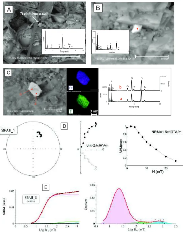
Font et al. (2014) applied paleo and rock magnetic methods in the SPA speleothem from

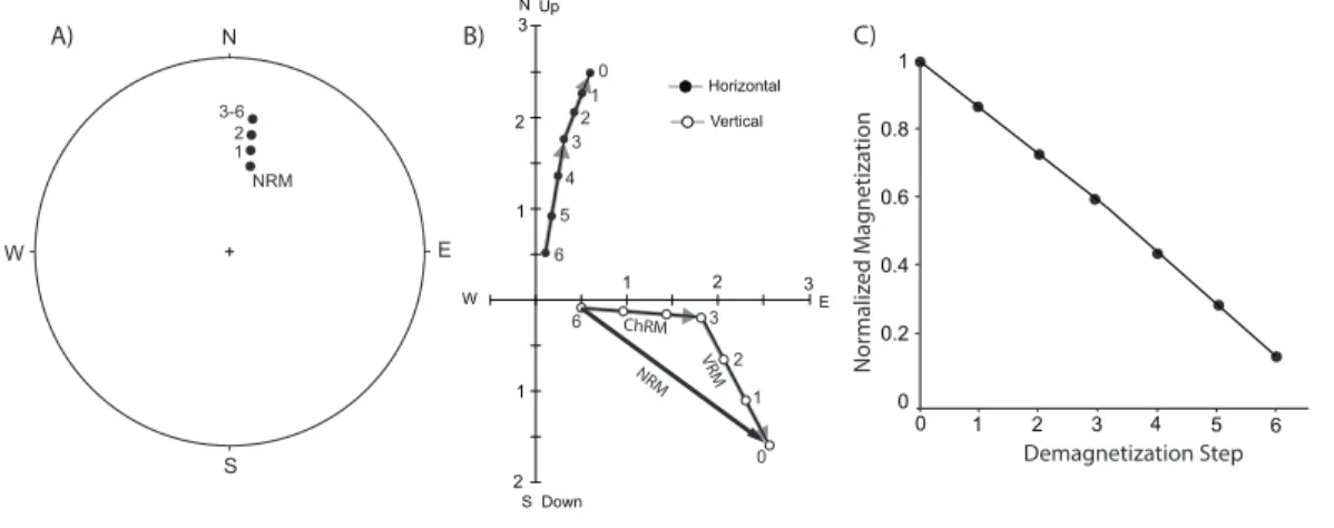
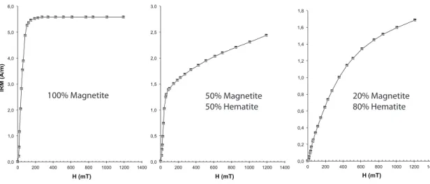
Algarve (Portugal) studied here. The results show that the main magnetic carrier is detrital titanomagnetite, identified by microscopic observation (Scanning Electron Microscopy (SEM) coupled to Energy Dispersive Spectra (EDS) composition) and magnetic properties (Cumulative Log-Gaussian (CLG) decomposition of IRM acquisition curves) (Figure 1.2). Comparison with the magnetic properties of the characteristic terra rossa soils capping the cave suggested that the detrital titanomagnetite is inherited from these terra soils and deposited in the speleothem’s surface by drip waters. This is comforted by the occurrence of magnetite grains observed in glass plates positioned below a drip water during 3 months (Figure 1.2A). The observation that magnetite is the main carrier of the NRM recorded in speleothems was also reported by: Osete et al., (2012), Strauss et al., (2013), Bourne et al., (2015), Jaqueto et al., (2016), Lascu et al., (2016), Zhu et al., (2017), Zanella et al., (2018) and Trindade et al., (2018), who identified magnetite by using several rock magnetic techniques (e.g. IRM, ARM, AF demagnetization, thermomagnetic curves) and scanning electroscopy. The main NRM mechanism is then a DRM, what together with stable magnetic directions (Figure 1.2), points the Algarve stalagmites as good candidates for paleo and environmental magnetic studies.

Despite the promising preliminary magnetic results in speleothems for paleomagnetic studies, some important aspects about the acquisition of magnetic remanence has not yet been well investigated. One of the possible problems pointed by some authors is related to the influence of the calcite growth dip angle in the recorded magnetic directions. They made a very simple test by comparing the obtained directions in central (horizontal layers) and lateral (vertical layers) samples, but the influence could not be confirmed. According to them, the differences observed in the magnetic directions between central and lateral samples are within the typical range of paleomagnetic measurement errors. However, the speleothems used in this study do not have a favourable shape for evaluating calcite dip effects since they are very thin and only 2/3 specimens could be sampled along the same growth lines. A different approach was conducted by Zhu et al. (2012), who studied the magnetic fabric of two speleothems. Similar directions of maximum principal axis of Anistropy of Isothermal Remanent Magnetization (AIRM) and NRM suggests that orientation of ferromagnetic minerals have been likely controlled by the geomagnetic field, and not by the orientation of calcite laminae growth.

Introduction

8

Figure 1.2 Scanning electron microscope (SEM) back-scattered images and EDS (Energy Dispersive Spectra) of a glass

plate positioned bellow a drip water during three months (A) and SPA stalagmite studied here (B-C), showing the presence of detrital Fe-Ti iron oxides, probably titanomagnetite. D) Stereographic and orthogonal projections of the magnetic direction obtained after Alternating Field demagnetization, as well as normalized magnetic intensity versus applied field H (mT), showing a stable and high intensity primary remanent magnetization. E) The decomposition of IRM acquisition curves using a Cumulative Log-Gaussian function shows the presence of a mixture of a low-coercivity (i.e. magnetite) and high coercivity (hematite) magnetic phases. (Modified from Font et al. (2014).

!

"

1.2.2 Contribution of speleothem magnetic archives in the calibration of Paleosecular variation records of the Earth’s magnetic field

Reconstruction of the ancient Earth’s magnetic field reconstructions is one of the most important challenge in geomagnetism to better understand the dynamics in the Earth’s core and the origin of the Earth’s magnetic field. More specifically, several models were developed during the last decade in order to reconstruct the high-frequency and short-term variations of the Earth’s magnetic field, called paleosecular variation (PSV), in the last 10-15 kyr. For example, Korte et al. (2011) and Nilsson et al. (2014) proposed the CALS10k.1b and pfmk models, respectively, for which reconstruction is based on archaeomagnetic, lava and sediment data of the last 10,000 years. Recently, Pavón-Carrasco et al. (2014) discarded sediment data, but used new data sets from volcanic and archaeological materials to propose the SHA.DIF.14k model for the last 14.000 years.

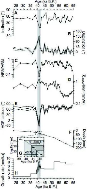
One of the greatest speleothem’s advantages is the possibility to obtain high-resolution paleomagnetic records, which allow documenting high-frequency instabilities of the geomagnetic field (in timescales of few years). For example, Osete et al. (2012) not only identified for the first time the Blake geomagnetic excursion in a speleothem from northern Spain, but also managed to date the different phases of the excursion (Figure 1.3). Accurate timing of geomagnetic excursion is crucial for understanding the geodynamo processes and for magnetostratigraphic correlation. More recently, Lascu et al. (2016) reported a paleosecular variation record from a North American speleothem, showing a geomagnetic excursion within the age interval 42.25-39.7 kyrs BP, peaking at 41.1 kyrs BP, which has been identified as the Laschamp excursion (Figure 1.4). This is the first age bracketing of the Laschamp excursion using radioisotopic dating, which had already been reported before

using volcanic paleomagnetic data (40Ar/39Ar dating), with similar ages (between 40.7 and

41.3 kyrs BP), and other sedimentary and ice core records. This geomagnetic excursion corresponds to the most studied example of a geomagnetic excursion, since it coincides with the demise of Homo Neanderthalensis and to the Last Glacial Maximum and massive Mediteranean eruptions. Thus, precise determination of the timing and duration of the Laschamp excursion helps elucidating major scientific questions in diverse areas such as geology, paleoclimatology and anthropology. Zanella et al. (2017) presented a 10.000 yrs high-resolution paleosecular variation record from two cores of an Alpine flowstone, covering almost the entire Holocene (0.5 - 9 kyrs). Comparison with PSV models and data obtained from lavas and archaeomagnetic objects shows that the flowstone is an excellent

Introduction

10 record of the Earth’s magnetic field during the last 9.000 years (Figure 1.5), providing promising data both for the detection of short term variations of the geomagnetic field and for calibration of regional PSV curves, in time intervals where paleomagnetic data is scarce.

Trindade et al. (2018) report a unique geomagnetic record for the last ~1500 years combining

data of two well-dated speleothems from Brazil, located near the present day minimum of the geomagnetic South Atlantic Anomally (SAA). The SAA marks the position of the weakest geomagnetic field on Earth, and historical geomagnetic data from ship logs, observatories and satellites indicate that the area of the anomaly has been growing and migrating continuously westward. However, the origin and longevity of the SAA are still poorly understood given the scarcity of paleomagnetic data in the southern hemisphere. This work successfully describes the evolution of the SAA through the last 1500 years, confirming that fast geomagnetic field variations derived from SAA are a recurrent feature in the region. Magnetic directions are consistent with historical observations of the Earth’s magnetic field in the last 500 years and with model ARCH3K.1 for older periods (Figure 1.6), what validates the paleomagnetic data provided by the speleothems.

Figure 1.3 The Blake Geomagnetic excursion (with three phases B1, B2 and B3) recorded by a speleothem, here identified by quick shifts in the magnetic declination and inclination values (Figure from Osete et al., 2012).

Figure 1.4 Magnetic properties and chronology of the Laschamp excursion in the speleothem specimen studied from

Crevice Cave, Missouri (USA). A: Inclination. B: Declination. C: Relative paleointensity (NRM/ARM). D: Magnetic grain

size. E: Virtual geomagnetic pole (VGP) latitude. F: Age-depth model based on 230Th dates. G: Incremental chronology

(from confocal microscopy layer counting) across the Laschamp, anchored to radioisotopic dates. H: Speleothem growth rates from the radioisotopic (black) and incremental (gray) age models (Lascu et al., 2016).

Introduction

12 Figure 1.5 Speleothem data collected from Alpine speleothems, compared to paleomagnetic data from archaeomagnetic and volcanic sources and to PSV models (Zanella et al., 2017).

Figure 1.6 Paleomagnetic record from two speleothems from Brazil, compared with PSV models (Trindade et al., 2018).

1.2.3 Speleothem’s magnetism as a climate proxy

Speleothems have been used for past climate reconstructions using several proxies. Particularly, oxygen and carbon isotopes are widely used, and even a database (SISAL) has

been created resuming all speleothem δ18O and δ13C data collected worldwide

[Atsawawaranunt et al., 2018; Lechleitner et al., 2018]. On the other side, magnetic proxies in speleothems have been poorly used. Past climate reconstructions using magnetic susceptibility of cave sediments have been successfully correlated with records obtained from other proxies [Elwood et al., 2001; Elwood et al., 2004; Elwood and Gose, 2006], but

Introduction

14 magnetic parameters obtained from a speleothem has only been used for climate reconstruction recently [Bourne et al., 2015; Jaqueto et al., 2016; Zhu et al., 2017]. A significant positive correlation between ferromagnetic mineral concentration (quantified by IRM of the soft component, magnetite) and oxygen isotope values measured in a speleothem from Virginia, USA, has been detected by Bourne et al., (2015). According to the authors,

δ18O values in the cave site are controlled by seasonal precipitation: enriched 18O rain during

Summer enhanced production of pedogenic magnetite and results in high concentrations of magnetic minerals. Jaqueto et al., (2016) used a similar approach in stalagmites from Brazil, and suggested that more negative (positive) values of oxygen and carbon isotopes correspond to lower (higher) values of magnetic mineral content. In this region, higher isotopic values are interpreted as drier periods, suggesting that vegetation cover controls the magnetic input

in the cave: drier periods (higher δ18O and δ13C) drives less vegetation cover, more erosion

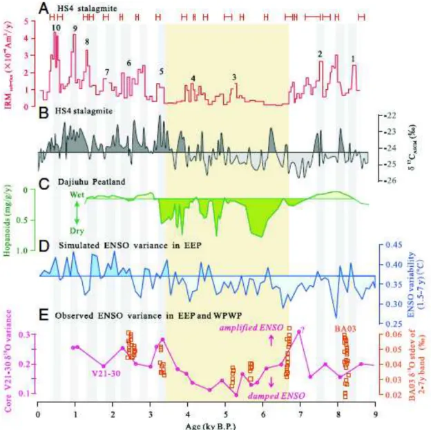
and therefore more transport of Fe-rich sediments into the cave resulting in higher magnetizations (and vice versa). Zhu et al., (2017) also used magnetic mineral concentration in Chinese speleothems to infer about rainfall amount: a high number of storms and consequent extreme rainfall events enhances the flux of pedogenic magnetite from soils to the cave, increasing magnetic mineral quantities. Since the frequency of storms in central China is correlated with El Niño Southern Oscillation (ENSO), the authors used the speleothem and its magnetic mineral content to study the variability of ENSO during the Holocene. As observed in Figure 1.7, high peaks in IRM of the soft component generally coincides with stronger ENSO periods (El Niño) and higher values of carbon isotopes, which is interpreted here as wetter periods.

Interpretation of climate proxies in speleothems is a very complex issue, and a multi-proxy approach has been suggested to improve the reliability and quality of the data [Fairchild et

al., 2012]. Speleothem magnetism brings new clue s to unravel past climate record, but still

Figure 1.7 Relationship of low-coercive magnetic mineral concentration with climate in central China: high-peaks in IRM soft componentes (A) correlates with higher (less negative) carbon isotope values and stronger ENSO periods, characterized by higher number of storms and consequent incresse in the amount of rainfall and extreme paleoflood events (Zhu et al., 2017).

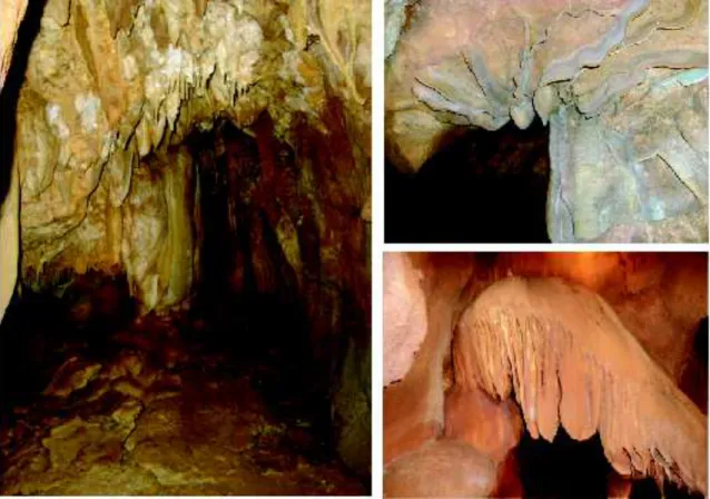
2.1 Speleothems

The studied rock formations during this PhD are speleothems (Figure 2.1). For this reason, starting with a general definition and a simple description of how they are formed is required. Speleothems are secondary mineral deposits formed by chemical precipitation of calcium

carbonate (CaCO3). They are generally found in karstic environments, characterized by

underground drainage systems, like sinkholes or caves, formed due to dissolution of soluble rocks such as limestones or dolomites, for example. Speleothem is the general term used to define all cave mineral deposits types. Stalactites, stalagmites, columns or flowstones are just a few examples of hundreds of variations of cave mineral deposits. The vast majority of

speleothems are composed by CaCO3, in form of calcite or aragonite crystals. The rainwater

becomes more acid, with lower pH, after reacting with soil’s CO2, according to the following

equation:

!!! ! ! !"!! ! !! !!!"!

As the acid water travels trough the calcium carbonate bedrock, it dissolves the rocks via the equation:

!"!#_{!! ! !}

!!"!! ! ! !"!!! !!!!!"!!

Once the water reaches the cave, it loses the CO2 through degassing to equilibrate the partial

pressure of CO2 in the cave atmosphere, which drives precipitation of CaCO3:

!"!!_{! !!!!!"!}!_{! ! ! !"!#!! !! !}

!! ! ! !"!!

Speleothems may grow through thousands of years, although not necessarily at the same rate. Over time, changes in climate, in the environment and morphology of the caves, water courses and several other factors may lead to variatiations in the speleothem’s growth rate. Some speleothems even present long hiatus in time and others have not grown to this day. If a speleothem section is cut, it is possible to observe the growth layers, similar to tree rings. Naturally, the growth layers age increase from the speleothem surface to the interior. Speleothems can be accurately dated at several growth layers, so that it is possible to estimate an age model for the whole speleothem. By collecting several data along a speleothem growth axis, it is possible to study its variation during a certain time interval with a very high resolution. For example, carbon or oxygen isotopic data profile provide important information about the past climate of the Earth since one of the most important factors controlling it is climate (temperature or amount of precipitation). In fact, speleothems are

Theoretical Principles

20 considered by scientific community as important climate archives of the Earth, but their potential does not end there. A few studies indicate that speleothems may also provide information about the past geomagnetic field, which is one of the major discussions during this PhD.

Figure 2.1 Photos of some mineral cave deposits (speleothems) from Excentricas Cave (Algarve, Portugal).

2.2 Geomagnetism

The main focus of my PhD is the magnetism in speleothems, particularly the reconstruction of the past Earth’s Magnetic Field. Thus, understanding the most basic definitions and equations in geomagnetism and paleomagnetism is required.

2.2.1 The Earth’s Magnetic Field

The first signs of the existence of a magnetic field on Earth were discovered by the Chinese about two thousand years ago when they realized that a magnet tended to align in the north-south direction. Since then, much about the Earth’s magnetic field has been discovered and documented. The surface geomagnetic field, H, can be defined as a three-dimensional vector

at any location on the Earth, characterized by a vertical (Hv) and horizontal (Hh) components, and an intensity as follows:

!!! ! !"# !

!! ! !!!"#!!!

Where I is the magnetic inclination, the angle of H with the horizontal plane. The horizontal

component is divided in the East (HE) and North (HN) components:

!! ! ! !"# ! !"#!!!!

!! ! ! !"# ! !"#!!!!

Where D is the magnetic declination, defined as the angle of Hh with the geographic north.

The total intensity is given by:

! ! !!!! !_!!! !_!!

Magnetic declination values range between 0º and 360º, positive clockwise, while magnetic inclination range between -90º and 90º, and is positive downward. The magnetic field direction is commonly described by its declination and inclination values. Figure 2.2 resumes the standard definition of the geomagnetic field.

The Earth’s magnetic field at the surface can be approximated by a magnetic field of a giant magnetic dipole located at the center of the Earth aligned with its rotational axis, which is called Geocentrical Axial Dipole (GAD) field. The present geomagnetic field is naturally more complex than the simple GAD model, attested by the fact that the real geomagnetic poles do not coincide with the geographic poles, as expected for the GAD model. For this reason, the model should be improved to an inclined geocentric dipole. The inclined GAD model that better describes the Earth’s present magnetic field has an angle of about 11.5º with the rotation axis, and explains around 80 to 90% of the surface magnetic field. The remaining part of the magnetic field is called the non-dipolar field, which is determined by subtracting the best-fitting inclined GAD approximation to the observed magnetic field.

Figure 2.2 Description of the magnetic field H (from Robert

Theoretical Principles

22 The geomagnetic field is continuously changing in several timescales, from milliseconds to millions of years. The shorter timescale variations are mainly due to currents in the ionosphere and magnetosphere. The solar wind, which carries charged particles, varies in density, temperature and speed, resulting in small diurnal fluctuations of the geomagnetic field at surface. Changes with timescales of one year or more are thought to reflect changes in the Earth’s interior, particularly in the outer core, and are referred as Paleosecular variation (PSV). It is generally accepted that electric currents due to convection (heating transfers) in the liquid outer core generate the geomagnetic field, but the knowledge about the origin of the Earth’s magnetic field is still in great development. The study of PSV is therefore object of intense research at present. Important geomagnetic field changes may also occurs in timescales of millions of years: geomagnetic reversals, when the north and south poles trade places, have been occurred several times in Earth’s history. How is it possible to know the existence of such events? They have been recorded in rocks. The study of the past geomagnetic field recorded in rocks has been object of intense research for a long time and is called paleomagnetism.

2.2.2 Magnetization in rocks

In paleomagnetism, one of the fundaments is that some rocks possess the ability to record the Earth Magnetic Field at the time they were formed. The first question is how does that happen. To answer this question, we need to understand the concept of magnetic dipole moment, or simply magnetic moment, M. The magnetic moment can be defined referring to a pair of magnetic charges or to a loop of electric current. In magnetization of rocks, it is convenient to consider the magnetic moment resulting from a pair of magnetic charges. So, the magnetic moment is proportional to the magnitude of charge m and an infinitesimal distance vector I between the plus and minus charges.

! ! !!!!!!!

When exposed to a magnetic field H, a force experienced by a magnetic charge with certain intensity and direction, the magnetic moment M tends to align with the magnetic field. The potential energy of this alignment is defined as follow:

! ! ! !!"!!"#$

Where ! is the angle between the magnetic moment M and the magnetic field H. Note that the minimum energy configuration is achieved when ! ! !", or, in another words, when M and H are parallel.

Almost all rocks in the Earth contain some ferromagnetic minerals, so they contain atoms with magnetic moments, which will align with the Earth Magnetic Field at the moment of the rock formation, when they are free to rotate. The total magnetization of a rock, J, is defined by the net magnetic moment per unit volume. In a single rock, J is calculated by the sum of the magnetic moments contained in the rock divided by its volume V:

! ! !_!!!

There are basically two types of magnetization: induced magnetization Ji and remanent

magnetization Jr. The induced magnetization is the magnetization acquired by a rock when

exposed to a magnetic field H. Ji is proportional to the magnetic susceptibility χ, which may

be interpreted as the “magnetizability” of the rock.

!! ! !!!

It results from the summed contributions of diamagnetic, paramagnetic and ferromagnetic materials composing the rock. Paramagnetic (diamagnetic) material acquires a weak magnetization in the same (contrary) direction of an external magnetic field, while it’s being applied, but loses the magnetization when the field is removed. Ferromagnetic minerals, usually dispersed in a paramagnetic or diamagnetic matrix of the rock, have a very high magnetic susceptibility. The magnetic susceptibility of a rock containing more than 0,1% of ferromagnetic minerals in the total volume is dominated by their fraction. Ferromagnetic minerals may also have the ability to keep the magnetization after the external field is removed, a characteristic responsible for the remanent magnetization of rocks.

The remanent magnetization Jr is the magnetization recording of the past magnetic fields that

have acted in the rock. When a magnetic field H applied in a rock is removed, the ferromagnetic minerals are able to keep the magnetization for a certain time t, on contrary to

paramagnetic or diamagnetic materials. After the magnetic field removal, Jr decays

exponentially, but depending on the magnetic grains size, it can be preserved through millions of years. Magnetic grains with diameters higher than 10 µm create several magnetic domains as it decreases magnetostatic energy, so that we refer to them as multi-domain (MD) grains. When magnetic grain size decreases, the number of magnetic domain decreases as well, until the grain becomes so small that dividing the grain in several magnetic domains is not energetically favorable anymore. In this case, the grain contains only one domain, and it is referred as a single-domain (SD) grain [Dunlop and Ozdemir, 1997; Liu et al., 2012].