odNEAT: an algorithm for decentralised online evolution of robotic controllers

Repositório ISCTE-IUL

Deposited in Repositório ISCTE-IUL:

2019-05-09

Deposited version:

Pre-print

Peer-review status of attached file:

Unreviewed

Citation for published item:

Silva, F., Urbano, P., Correia, L. & Christensen, A. L. (2015). odNEAT: an algorithm for decentralised online evolution of robotic controllers. Evolutionary Computation. 23 (3), 421-449

Further information on publisher's website:

10.1162/EVCO_a_00141

Publisher's copyright statement:

This is the peer reviewed version of the following article: Silva, F., Urbano, P., Correia, L. & Christensen, A. L. (2015). odNEAT: an algorithm for decentralised online evolution of robotic controllers. Evolutionary Computation. 23 (3), 421-449, which has been published in final form at https://dx.doi.org/10.1162/EVCO_a_00141. This article may be used for non-commercial purposes in accordance with the Publisher's Terms and Conditions for self-archiving.

Use policy

Creative Commons CC BY 4.0

The full-text may be used and/or reproduced, and given to third parties in any format or medium, without prior permission or charge, for personal research or study, educational, or not-for-profit purposes provided that:

• a full bibliographic reference is made to the original source • a link is made to the metadata record in the Repository • the full-text is not changed in any way

The full-text must not be sold in any format or medium without the formal permission of the copyright holders.

Serviços de Informação e Documentação, Instituto Universitário de Lisboa (ISCTE-IUL) Av. das Forças Armadas, Edifício II, 1649-026 Lisboa Portugal

Online Evolution of Robotic Controllers

Fernando Silva

Bio-inspired Computation and Intelligent Machines Lab, 1649-026 Lisboa, Portugal Instituto de Telecomunicac¸ ˜oes, 1049-001 Lisboa, Portugal

LabMAg, Faculdade de Ciˆencias, Universidade de Lisboa, 1749-016 Lisboa, Portugal

Paulo Urbano

LabMAg, Faculdade de Ciˆencias, Universidade de Lisboa, 1749-016 Lisboa, Portugal

Lu´ıs Correia

LabMAg, Faculdade de Ciˆencias, Universidade de Lisboa, 1749-016 Lisboa, Portugal

Anders Lyhne Christensen

Instituto Universit´ario de Lisboa (ISCTE-IUL), 1649-026 Lisboa, Portugal

Abstract

Online evolution gives robots the capacity to learn new tasks and to adapt to chang-ing environmental conditions durchang-ing task execution. Previous approaches to online evolution of neural controllers are typically limited to the optimisation of weights in networks with a pre-specified, fixed topology. In this article, we propose a novel ap-proach to online learning in groups of autonomous robots called odNEAT. odNEAT is a distributed and decentralised neuroevolution algorithm that evolves both weights and network topology. We demonstrate odNEAT in three multirobot tasks: aggrega-tion, integrated navigation and obstacle avoidance, and phototaxis. Results show that odNEAT approximates the performance of rtNEAT, an efficient centralised method, and outperforms IM-(µ + 1), a decentralised neuroevolution algorithm. Compared with rtNEAT and IM-(µ + 1), odNEAT’s evolutionary dynamics lead to the synthesis of less complex neural controllers with superior generalisation capabilities. We show that robots executing odNEAT can display a high degree of fault tolerance as they are able to adapt and learn new behaviours in the presence of faults. We conclude with a series of ablation studies to analyse the impact of each algorithmic component on performance.

Keywords

Artificial neural networks, decentralised algorithms, multirobot systems, neurocon-troller, online evolution.

1

Introduction

Evolutionary computation has been widely studied and applied as a means to au-tomate the design of robotic systems (Floreano and Keller, 2010). In evolutionary robotics, controllers are typically based on artificial neural networks (ANNs). The pa-rameters of the ANNs, such as the connection weights and occasionally the topology, are optimised by an evolutionary algorithm, a process termed neuroevolution.

Neu-roevolution has been successfully applied to tasks in a number of domains, see Yao (1999) and Floreano et al. (2008) for examples.

In traditional evolutionary approaches, controllers are synthesised offline. When a suitable neurocontroller is found, it is transferred to real robots. Once deployed, the controllers are thus specialised to a particular task and environmental conditions. Even if the controllers are based on adaptive neural models (Beer and Gallagher, 1992; Harvey et al., 1997), they are fixed solutions and exhibit limited capacity to adapt to conditions not seen during evolution.

Online evolution is a process of continuous adaptation that potentially gives robots the capacity to respond to changes and unforeseen circumstances by modifying their behaviour. An evolutionary algorithm is executed on the robots themselves while they perform their tasks. The main components of the evolutionary algorithm (evaluation, selection, and reproduction) are carried out autonomously on the robots without any external supervision. This way, robots have the potential for long-term self-adaptation in a completely autonomous manner. The first example of online evolution in a real mo-bile robot was performed by Floreano and Mondada (1994). A contribution by Watson et al. (1999, 2002) followed, in which the use of multirobot systems was motivated by an anticipated speed-up of evolution due to the inherent parallelism in such systems.

Over the last decade, different approaches to online evolution in multirobot sys-tems have been developed, see for instance Bianco and Nolfi (2004); Bredeche et al. (2009); Haasdijk et al. (2010); Prieto et al. (2010); Karafotias et al. (2011). Notwithstand-ing, in such contributions, online approaches have been limited to the evolution of weighting parameters in fixed-topology ANNs. Fixed-topology methods require the system designer to decide on a suitable topology for a given task, which usually in-volves intensive experimentation. A non-optimal topology affects the evolutionary process and, consequently, the potential for adaptation.

In this article, we present a novel algorithm for online evolution of ANN-based controllers in multirobot systems called Online Distributed NeuroEvolution of Aug-menting Topologies (odNEAT). odNEAT is completely decentralised and can be dis-tributed across multiple robots. odNEAT is characterised by maintaining genetic diver-sity, protecting topological innovations, keeping track of poor solutions to the current task in a tabu list, and exploiting the exchange of genetic information between robots for faster adaptation. Moreover, robots executing odNEAT are flexible and potentially fault-tolerant, as they can adapt to new environmental conditions and to changes in the task requirements.

This article offers a comprehensive presentation and analysis of odNEAT, initially introduced in Silva et al. (2012). To the best of our knowledge, only one other online method that optimises neural topologies and weights in a decentralised manner has previously been proposed; the island model-based (µ + 1) algorithm of Schwarzer et al. (2011), henceforth IM-(µ + 1) — an implementation of the (µ + 1)-online algorithm by Haasdijk et al. (2010) with hoc transmissions of randomly chosen controllers. In ad-dition, the real-time NeuroEvolution of Augmenting Topologies (rtNEAT) algorithm by Stanley et al. (2005), an online version of NeuroEvolution of Augmenting Topolo-gies (NEAT) (Stanley and Miikkulainen, 2002) designed for video games, is a promi-nent centralised evolutionary algorithm that has a number of features in common with odNEAT. The goal of rtNEAT is similar to that of odNEAT in online evolution. rtNEAT was developed to allow non-player characters to optimise their behaviour during a game. We experimentally compare the performance of odNEAT with the performance of rtNEAT and IM-(µ + 1) in three simulation-based experiments involving groups of

e-puck-like robots (Mondada et al., 2009). The first experiment, the aggregation task, requires individual search and coordinated movement to form and remain in a sin-gle group. The task is challenging given the robots’ limited sensing capabilities. The second experiment, the integrated navigation and obstacle avoidance task, is used as a means to analyse odNEAT’s behaviour when two conflicting objectives have to be learned. The task implies an integrated set of actions, and consequently a trade-off between avoiding obstacles and maintaining speed and forward movement. The third experiment, the phototaxis task, is performed in a dynamic environment with changing task parameters. The main conclusion is that odNEAT is an efficient and robust online neuroevolution algorithm. odNEAT yields performance levels comparable to rtNEAT, despite being completely decentralised, and odNEAT significantly outperforms IM-(µ + 1). We furthermore show that: (i) odNEAT allows robots to continuously adapt to different environmental conditions and to the presence of faults injected in the sensors, and that (ii) odNEAT evolves controllers with relatively low complexity and superior generalisation performance.

The article is organised as follows. In Section 2, we discuss previous studies on on-line evolution in multirobot systems, and we introduce NEAT, rtNEAT, and IM-(µ + 1). In Section 3, we present and motivate the features of odNEAT. In Section 4, we explain our experimental methodology and the three tasks used in this study. In Section 5, we present and discuss our experimental results. Section 6 is dedicated to the exploration and analysis of odNEAT in terms of long-term self-adaptation, fault tolerance, and the influence of each algorithmic component on performance. Concluding remarks and directions for future research are provided in Section 7.

2

Background and Related Work

In this section, we review the main approaches in the literature for online evolution of ANN-based controllers in multirobot systems, and the main characteristics of NEAT, rtNEAT, and IM-(µ + 1).

2.1 Online Evolutionary Robotics

Existing approaches to online evolution in multirobot systems fall into three cate-gories (Eiben et al., 2010a): (i) distributed evolution, (ii) encapsulated evolution, and (iii) a hybrid approach, similar to a physically distributed island model.

2.1.1 Distributed Evolution

In distributed evolution, each robot carries a single genotype. The evolutionary process takes place when robots meet and exchange genetic information. The first attempt at truly autonomous continuous evolution in multirobot systems was performed by Wat-son et al. (1999, 2002), and entitled embodied evolution. Robots probabilistically broad-cast a part of their stochastically mutated genome at a rate proportional to their fit-ness. Robots that receive gene transmissions incorporate this genetic material into their genome with a probability inversely proportional to their fitness. This way, selection and variation operators are implemented in a distributed manner through the interac-tions between robots.

Following Watson et al.’s initial publications on embodied evolution, a number of improvements and extensions were proposed, see Bianco and Nolfi (2004) and Karafo-tias et al. (2011) for examples. The distribution of an evolutionary algorithm in a pop-ulation of autonomous robots offered the first demonstration of evolution as a contin-uous adaptation process. The main disadvantage of embodied evolution approaches

is that the improvement of existing solutions is only based on the exchange of genetic information between robots. In large and open environments, where encounters may be rare or frequent transmission of information may be infeasible, the evolutionary process is thus prone to stagnation.

2.1.2 Encapsulated Evolution

A complementary approach, encapsulated evolution, overcomes stagnation as each robot maintains a population of genotypes stored internally and runs its self-sufficient instance of the evolutionary algorithm locally. Alternative controllers are executed se-quentially and their fitness is measured. Within this paradigm, robots adapt individu-ally without interacting or exchanging genetic material with other robots.

In order to enable efficient encapsulated evolution, Bredeche et al. (2009) proposed the (1+1)-online algorithm after the classic (1+1)-evolutionary strategy. Montanier and Bredeche (2011) then extended the (1+1)-online algorithm to incorporate a restart pro-cedure as a means to bypass local optima. In-between the two studies, Haasdijk et al. (2010) proposed the (µ + 1)-online algorithm. The algorithm was evaluated for the ability to address noisy evaluation conditions and to produce solutions within a satis-factory period of time. With respect to Haasdijk et al.’s algorithm, subsequent studies examined: (i) distinct self-adaptive mechanisms for controlling the mutation opera-tor (Eiben et al., 2010b), (ii) racing as a technique to cut short the evaluation of poor individuals (Haasdijk et al., 2011), and (iii) the impact of a number of parameters on performance (Haasdijk et al., 2012). Although there has been a number of successive contributions using encapsulated evolution, the main drawback of the approach is that there is no transfer of knowledge or exchange of genetic information between robots, which can accelerate online evolution (Huijsman et al., 2011).

2.1.3 Hybrid Evolution

The two methodologies, encapsulated evolution and distributed evolution, can be com-bined, leading to a hybrid approach similar to an island model. Each robot optimises the internal population of genomes through intra-island variation, and genetic infor-mation between two or more robots is exchanged through inter-island migration.

Distinct approaches to hybrid online evolution have been proposed. An example of such a method is the one introduced by Elfwing et al. (2005), in which task-oriented and survival-oriented criteria are combined. In the approach, robots evaluate their in-ternal population of solutions in a time-sharing manner. During the evaluation period, the performance of a controller is assessed based on its ability to solve the task and to sustain the robot’s energy reserve by finding and replacing battery packs.

With the purpose of enabling online self-organisation of behaviour in multirobot systems, Prieto et al. (2010) proposed the real-time Asynchronous Situated Coevolution (r-ASiCo) algorithm. r-ASiCo is based on a reproduction mechanism in which individ-ual robots carry an embryo. When robots meet, the embryo is genetically modified. If a controller is unable to solve the task, the embryo is used to produce a new controller. Huijsman et al. (2011) introduced an approach based on the encapsulated (µ + 1)-online algorithm, and on a peer-to-peer evolutionary algorithm designed by Laredo et al. (2010). The hybrid method consistently yielded a better performance than both pure distributed evolution and pure encapsulated evolution, due to its ability to lever-age parallelism in multirobot systems. Despite the new approaches and algorithmic advances, one of the main limitations of existing approaches to online evolution, in-cluding all methods described above, is that neuroevolution solely adjusts the weights of the ANN, while the topology must be specified a priori by the experimenter and

remains fixed during task execution.

2.2 NeuroEvolution of Augmenting Topologies

The NeuroEvolution of Augmenting Topologies (NEAT) method (Stanley and Miikku-lainen, 2002) is one of the most prominent offline neuroevolution algorithms. NEAT optimises both network topologies and weighting parameters. NEAT executes with global and centralised information like canonical evolutionary algorithms, and has been successfully applied to distinct problems, outperforming several methods that use fixed-topologies (Stanley and Miikkulainen, 2002; Stanley, 2004). The high performance of NEAT is due to three key features: (i) the tracking of genes with historical markers to enable meaningful crossover between networks with different topologies, (ii) a nich-ing scheme that protects topological innovations, and (iii) the incremental evolution of topologies from simple initial structures, i.e., complexification.

In NEAT, the network connectivity is represented through a flexible genetic en-coding. Each genome contains a list of neuron genes and a list of connection genes. Connection genes encompass: (i) references to the two neuron genes being connected, (ii) the weight of the connection gene, (iii) one bit indicating if the connection gene should be expressed or not, and (iv) a global innovation number, unique for each gene in the population. Innovation numbers are assigned sequentially, and they therefore represent a chronology of the genes introduced. Genes that express the same feature are called matching genes. Genes that do not match are either disjoint or excess, depend-ing on whether they occur within or outside the range of the other parent’s innovation numbers. When crossover is performed, matching genes are aligned. The NP-hard problem of matching distinct network topologies is thus avoided and crossover can be performed without a priori topological analysis. In terms of mutations, NEAT allows for classic connection weight and neuron bias perturbations, and structural changes that lead to the insertion of either a new connection between two previously uncon-nected neurons, or a new neuron. A new neuron gene, representing the new neuron in the ANN, is introduced in the genome by splitting an old connection gene into two new connection genes.

NEAT protects new structural innovations by reducing competition between genomes representing differing structures and network complexities. The niching scheme is composed of speciation and fitness sharing. Speciation divides the popula-tion into non-overlapping sets of similar genomes based on the amount of evolupopula-tionary history they share. Explicit fitness sharing dictates that individuals in the same species share the fitness of their niche. The fitness scores of members of a species are first ad-justed, i.e., divided by the number of individuals in the species. Species then grow or shrink in size depending on whether their average adjusted fitness is above or below the population average. Since the size of the species is taken into account in the compu-tation of the adjusted fitness, new smaller species are not discarded prematurely, and one species does not dominate the entire population.

NEAT starts with a population of simple networks with no hidden neurons. New neurons and new connections are then progressively added to the networks as a re-sult of structural mutations. Because NEAT speciates the population, the algorithm effectively maintains a variety of networks with different structures and different com-plexities over the course of evolution. In this way, NEAT can search for an appropriate degree of complexity to the current task.

2.3 rtNEAT: Real-time NEAT

Real-time NeuroEvolution of Augmenting Topologies (rtNEAT) was introduced by Stanley et al. (2005) with the purpose of evolving ANNs online. rtNEAT is a cen-tralised real-time version of NEAT originally designed for video games. Compared with NEAT, rtNEAT differs in a number of aspects, namely: (i) rtNEAT is a steady-state algorithm, while NEAT is generational, (ii) rtNEAT produces one offspring at regular intervals, every n time steps, and (iii) unlike NEAT, in which the number of species may vary, rtNEAT attempts to keep the number of species constant. To that end, rtNEAT adjusts a threshold Ctthat determines the degree of topological similarity

necessary for individuals to belong to a species. When there are too many species, Ct

is increased to make species more inclusive; when there are too few, Ctis decreased to

make species less inclusive. Despite these differences, rtNEAT has shown to preserve the dynamics of NEAT, namely complexification and protection of innovation through speciation (Stanley et al., 2005).

Even though rtNEAT only creates one offspring at a time, it approximates NEAT’s behaviour, in which a number of offspring nkis assigned to each species. In rtNEAT, a

parent species Skis chosen proportionally to its average adjusted fitness, as follows:

P r(Sk) =

Fk

Ftotal

(1) where Fkis the average adjusted fitness of species k, and Ftotalis the sum of all species’

average adjusted fitness. As a result, the expected number of offspring for each species in rtNEAT is, over time, proportional to nkin traditional NEAT. The remaining process

of reproduction is similar to NEAT’s: two parents are chosen, and crossover and mu-tation operators are applied probabilistically. The individual with the lowest adjusted fitness is then removed from the population and replaced with the new offspring.

Similarly to rtNEAT, odNEAT is based on steady-state dynamics. We therefore use rtNEAT instead of the original, generational NEAT for comparisons of features and performance in the remainder of the article.

2.4 IM-(µ + 1) algorithm

To the best of our knowledge, only one method has previously been pro-posed (Schwarzer et al., 2011) that optimises both the weighting parameters and the topology of ANN-based controllers according to a physically distributed island model. The algorithm is a variant of the (µ + 1)-online algorithm, proposed by Haasdijk et al. (2010), with random ad-hoc exchange of genomes between robots. We henceforth refer to this method as IM-(µ + 1). We first describe the similarities between IM-(µ + 1) and rtNEAT, and then the execution loop of IM-(µ + 1).

The IM-(µ + 1) algorithm mimics a number of features of rtNEAT. Firstly, new genes are assigned innovation numbers. An important difference with respect to rt-NEAT is that in IM-(µ + 1), innovation numbers are local and randomly chosen from a predefined interval to enable a decentralised implementation. The interval [1, 1000] was used in Schwarzer et al. (2011). Secondly, as in rtNEAT, crossover is performed between similar genomes to maximise the chance of producing meaningful offspring. Explicit speciation is not used in IM-(µ + 1). Instead, genomes that have a high degree of genetic similarity are recombined. Genetic similarity is computed based on the ratios of matching connection genes and matching neuron genes.

Thirdly, IM-(µ + 1) follows rtNEAT’s complexification policy and usually starts evolution from simple topologies, although it can be seeded with a parametrisable

number of hidden neurons (Schwarzer et al., 2011). IM-(µ+1) allows for non-structural mutations similarly to rtNEAT, namely connection weight and neuron bias perturba-tions, but it employs different methods for optimising the topology of the ANN. Struc-tural mutation of a connection gene can either remove the gene or introduce a new connection gene in a random location and with a randomly assigned weight. In the same way, structural mutation of a neuron gene can either delete the gene or produce a new neuron gene with a random innovation number and a random bias value. In ad-dition, insertion of new neuron genes and connection genes can be performed through duplication and differentiation of an existing neuron gene, and of its incoming and outgoing connection genes.

2.4.1 Execution Loop

In the IM-(µ + 1) algorithm, as in the encapsulated (µ + 1)-online, each robot maintains an internal population of µ genomes. Robots in close proximity can exchange genomes according to a migration policy that presupposes bilateral and synchronous commu-nication. When two robots meet, they exchange genomes if none of them has had a migration within a predefined period of time. Each robot randomly selects and re-moves one genome from its internal population, and probabilistically applies crossover and mutation. The resulting genome is transmitted to the neighbouring robot, and the genome received is incorporated in the internal population.

During task execution, λ = 1 new offspring is produced at regular time intervals. One genome from the population of µ genomes maintained by the robot is randomly selected to be a parent. A second parent is used if there is any genome in the popu-lation considered genetically similar. The offspring resulting from crossover and mu-tation is decoded into an ANN that controls the robot. The controller operates for a fixed amount time called the evaluation period. When the evaluation period elapses, the evaluated genome is added to the population of the robot. The genome with the lowest fitness score is subsequently removed to keep the population size constant.

3

odNEAT

In this section, we present Online Distributed NeuroEvolution of Augmenting Topolo-gies (odNEAT), an online neuroevolution algorithm for multirobot systems, in which both the weighting parameters and the topology of the ANNs are under evolutionary control. One of the motivations behind odNEAT is that, by evolving neural topologies, the algorithm bypasses the inherent limitations of fixed-topology online algorithms. As in rtNEAT, odNEAT starts with simple controllers, in which the input neurons are connected to the output neurons. The ANNs are progressively augmented with new neurons and new connections, and a suitable network topology is the product of a continuous evolutionary process. In addition, odNEAT is distributed across multiple robots that evolve in parallel and exchange solutions.

odNEAT adopts rtNEAT’s matching and recombination of neural topologies, and niching scheme, and presents a number of differences when compared with IM-(µ + 1). The differences between the three algorithms are summarised in Table 1. odNEAT differs from rtNEAT and IM-(µ + 1) in a number of key aspects, the most significant being:

• The internal population of each robot is constructed in an incremental manner. • odNEAT maintains a local tabu list of recent poor solutions, which enables a robot

• odNEAT follows a unilateral migration policy for the exchange of genomes be-tween robots. Copies of the genome encoding the active controller are probabilis-tically transmitted to nearby robots if they have a competitive fitness score and represent topological innovations with respect to the robot’s internal population of solutions.

• odNEAT uses local, high-resolution timestamps. Each robot is responsible for as-signing a timestamp to each local innovation, be it a new connection gene or a new neuron gene. The use of high-resolution timestamps for labels practically guaran-tees uniqueness and allows odNEAT to retain the concept of chronology.

• A controller remains active as long as it is able to solve the task. A new controller is only synthesised if the current one fails, i.e., when it is actually necessary. • New controllers are given a minimum amount of time controlling the robot, a

mat-uration period.

Table 1: Summary of the main differences between odNEAT, rtNEAT, and IM-(µ + 1)

odNEAT rtNEAT IM-(µ + 1)

Population Distributed Centralised Distributed

Niching scheme Yes Yes No

Tabu list Yes No No

Migration policy Unilateral n/a Synchronous

Innovation numbers High-res. timestamps Sequential Random

Controller replacement When previous fails Periodically Periodically

Maturation period Yes No No

3.1 Measuring Individual Performance

In odNEAT, robots maintain a virtual energy level reflecting the individual task per-formance of the current controller. Controllers are assigned a default and domain-dependent virtual energy level when they start executing. The energy level increases and decreases as a result of the robot’s behaviour. If a controller’s energy level reaches a minimum threshold, a new controller is produced.

One common issue, especially for highly complex tasks, is that online evaluation is inherently noisy. Very dissimilar conditions may be presented to different genomes when they are translated into a controller and evaluated. The location of a robot within the environment and the proximity to other robots, for instance, are factors that may have a significant influence on performance and behaviour. With the purpose of obtain-ing a more reliable fitness estimate, odNEAT distobtain-inguishes between the fitness score of a solution and its current energy level. The fitness score is defined as the average of the virtual energy level, sampled at regular time intervals.

3.2 Internal Population, Exchange of Genomes, and Tabu List

In odNEAT, each robot maintains a local set of genomes in an internal population. The internal population is subject to speciation and fitness sharing. The population contains genomes generated by the robot, namely the current genome and previously active genomes that have competitive fitness scores, and genomes received from other robots. Every control cycle, a robot probabilistically broadcasts a copy of its active genome and

the corresponding virtual energy level to robots in its immediate neighbourhood, an inter-robot reproduction event, with a probability computed as follows:

P (event) = Fk Ftotal

(2) where Fkis the average adjusted fitness of local species k to which the genome belongs

and Ftotal is the sum of all local species’ average adjusted fitnesses. The broadcast

probability promotes the propagation of topological innovations with a competitive fitness.

The internal population of each robot is updated according to two principles. Firstly, a robot’s population does not allow for multiple copies of the same genome. Due to the exchange of genetic information between the robots, a robot may receive a copy of a genome that is already present in its population. Whenever a robot receives a copy C’ of a genome C, the energy level of C’ is used to incrementally average the fitness of C, and thus to provide the receiving robot with a more reliable estimate of the genome’s fitness. Secondly, whenever the internal population is full, the insertion of a new genome is accompanied by the removal of the genome with the lowest adjusted fitness score. If a genome is removed or added, the corresponding species has either increased or decreased in size, and the adjusted fitness of the species is recalculated.

Besides the internal population, each robot also maintains a local tabu list, a short-term memory which keeps track of recent poor solutions, namely: (i) genomes removed from the internal population because it got full, or (ii) genomes whose virtual energy level reached the minimum threshold, and therefore failed to solve the task. In the latter case, the genome is added to the tabu list but it is maintained in the internal population as long as its fitness is comparatively competitive.

The tabu list filters out solutions broadcast by other robots that are similar to those that have already failed. The purpose of the tabu list is: (i) to avoid flooding the internal population with poor solutions, and (ii) to keep the evolutionary process from cycling around in an unfruitful neighbourhood of the solution space. Received genomes must first be checked against the tabu list before they become part of the internal population. Received genomes are only included in the internal population if they are topologically dissimilar from all genomes in the tabu list.

3.3 New Genomes and the Maturation Period

When the virtual energy level of a controller reaches the minimum threshold, because it is incapable of solving the task, a new genome is created. In this process, an intra-robot reproduction event, a parent species is chosen proportionally to its average adjusted fitness, as defined in (2). Two parents are selected from the species, each one via a tour-nament selection of size 2. The offspring is created based on crossover of the parents’ genomes and mutation of the new genome. Once the new genome is decoded into a new controller, it is guaranteed a maturation period during which no controller re-placement takes place. The new controller can continue to execute after the maturation period if its energy level is above the threshold.

odNEAT’s maturation period is conceptually similar to the recovery period of the (1 + 1)-online algorithm (Bredeche et al., 2009), and its purpose is twofold. Firstly, the maturation period is important because the new controller may be an acceptable so-lution to the task but the environmental conditions in which it starts to execute may be unfavourable. Thus, the new controller is protected for a minimum period of time.

Secondly, the maturation period defines a lower bound of activity in the environment that should be sufficiently long to enable a proper estimate of the quality of the con-troller. This implies a trade-off between a minimum evaluation time and how many candidate solutions can be evaluated within a given amount of time. A longer matu-ration period increases the reliability of the fitness estimate of solutions that fail, i.e., of the stepping stones of the evolutionary process, while a shorter maturation period increases the number of solutions that can be evaluated within a given period of time. In Algorithm 1, we summarise odNEAT as executed by each robot.

Algorithm 1Pseudo-code of odNEAT that runs independently on every robot. The ex-perimental parameters of odNEAT and the robot capabilities are detailed in Section 4.1

genome ← create random genome() controller ← assign as controller(genome) energy ← default initial energy

loop

if broadcast? then

send(genome, robots in communication range)

end if

if has received? then

for all c in received genomes do

if tabu list approves(c) and population accepts(c) then

add to population(c) adjust population size() adjust species fitness()

end if end for end if

operate in environment() energy ← update energy level()

if energy ≤ minimum energy threshold and not(in maturation period?) then

add to tabu list(genome) offspring ← generate offspring() update population(offspring)

genome ← replace genome(offspring) controller ← assign as controller(genome) energy ← default initial energy

end if end loop

4

Experimental Methodology

In this section, we define our experimental methodology, including the simulation plat-form and robot model, and we describe the three tasks used in the study: aggregation, phototaxis, and integrated navigation and obstacle avoidance. Our experiments serve as a means to determine if and how odNEAT evolves controllers for solving the spec-ified tasks, the complexity of solutions evolved, and the efficiency of odNEAT when compared with rtNEAT and IM-(µ + 1).

4.1 Experimental Setup

We use JBotEvolver (Duarte et al., 2014) to conduct our simulated experiments. JBotE-volver is an open-source, multirobot simulation platform, and neuroevolution frame-work. The simulator is written in Java and implements 2D differential drive kinematics.

In our experimental setup, the simulated robots are modelled after the e-puck (Mondada et al., 2009), a 7.5 cm in diameter differential drive robot capable of moving at speeds up to 13 cm/s. Each robot is equipped with infrared sensors that multiplex obstacle sensing and communication between robots at a range of up to 25 cm.1 _{The sensors of the robots are used in the three tasks to detect walls and other}

robots. In real e-pucks, the wall sensors can be implemented with active infrared sen-sors, while the robot sensors can be implemented using the e-puck range & bearing board (Guti´errez et al., 2008). In the phototaxis task, robots are also given the ability to detect the light source, which can be provided by the fly-vision turret or by the omni-directional vision turret.2 Each sensor and each actuator are subject to noise, which is simulated by adding a random Gaussian component within ±5% of the sensor satura-tion value or actuasatura-tion value. Each robot also has an internal sensor that enables it to perceive its current virtual energy level.

Each robot is controlled by an ANN produced by the evolutionary algorithm be-ing tested. The controllers are discrete-time recurrent neural networks with connec-tion weights ∈ [−10, 10]. The inputs of the ANN are the normalised readings ∈ [0, 1] from the sensors mentioned above. The output layer has two neurons, whose values are linearly scaled from [0, 1] to [−1, 1]. The scaled output values are used to set the signed speed of each wheel (positive in one direction, negative in the other). The acti-vation function is the logistic function. The three algorithms start with simple networks with no hidden nodes, and with each input neuron connected to every output neuron. Evolution is therefore responsible for adding new neurons and new connections, both feed-forward and recurrent.

A group of five robots operates in a square arena surrounded by walls. The size of the arena was chosen to be 3 x 3 meters. Every 100 ms of simulated time, each robot executes a control cycle. In Table 2, we summarise the characteristics common to the three tasks. Regarding the configuration of the evolutionary algorithms, the parame-ters are the same for odNEAT, rtNEAT, and IM-(µ + 1): crossover rate - 0.25, mutation rate - 0.1, add neuron rate - 0.03, add connection rate - 0.05, and weight mutation mag-nitude - 0.5. The parameters were found experimentally: new connections have to be added more frequently than new neurons, and evolution tends to perform better if neural networks are recombined and augmented in a parsimonious manner. odNEAT is configured with a maturation period of 5 control cycles (50 seconds). Preliminary experiments showed this parameter value to provide an appropriate trade-off between the reliability of fitness estimates and the speed of convergence towards good solu-tions. A previously found to be poor solution is removed from the tabu list if a similar genome is not among the last 50 genomes received by the robot. Performance is robust to moderate variations in the parameters.

4.2 Preliminary Performance Tuning

We conducted a series of preliminary tests across all three tasks as a means to analyse the algorithms’ dynamics. Firstly, we tested both odNEAT and rtNEAT with: (i) a dynamic compatibility threshold and a target number of species from 1 to 10, and (ii) a fixed compatibility threshold δ = 3.0 for speciating the population, with corresponding coefficients set as in previous studies using NEAT (Stanley and Miikkulainen, 2002;

1_{The original e-puck infrared range is 2-3 cm (Mondada et al., 2009). In real e-pucks, the liblrcom library,}

available at http://www.e-puck.org, extends the range up to 25 cm and multiplexes infrared communi-cation with proximity sensing.

Table 2: Summary of the experimental details

Group size 5 robots

Broadcast range 25 cm

Control cycle frequency 100 ms

Arena size 3 x 3 meters

Simulation length 100 hours

Runs per configuration 30

odNEAT population size 40 genomes per internal population IM-(µ + 1) population size 40 genomes per internal population

rtNEAT population size 200 genomes

Neural network weight range [-10, 10]

Inputs range [0,1]

Outputs range [0,1], rescaled to [-1, 1]

Activation function Logistic function

Stanley, 2004). Results were found to be similar, and we therefore decided to use a fixed compatibility threshold.

Secondly, we verified that the periodic production of new controllers in rtNEAT and in IM-(µ + 1) led to incongruous group behaviour. Regular substitution of con-trollers caused the algorithms to perform poorly in collective tasks that explicitly re-quired continuous group coordination and cooperation, such as the aggregation task. In IM-(µ + 1), ruptures of collective behaviour were caused by having every robot changing to a new controller at the same time. In rtNEAT, rupture of collective be-haviour was still significant but less accentuated, as only one controller was substituted at regular time intervals. We compared the average fitness score of consecutive groups of controllers executed on the robots. In the majority of the substitutions, the perfor-mance of new controllers was worse than the perforperfor-mance of the previous ones. In these cases, differences in the fitness scores were statistically significant in the aggre-gation task for rtNEAT and for IM-(µ + 1) (ρ < 0.01, Mann-Whitney test), and in the phototaxis task for IM-(µ + 1) (ρ < 0.05).

To provide a fair and meaningful comparison of performance, we modified the condition for creating new offspring. rtNEAT and IM-(µ + 1) were modified to pro-duce offspring when a robot’s energy level reaches the minimum threshold (zero in our experiments), i.e., when a new controller is necessary. In the IM-(µ + 1) algorithm, we also observed collisions in the assignment of innovation numbers. To reduce the chance of collisions, we replaced the random assignment of innovation numbers by high-resolution timestamps, as in odNEAT. We verified that the modified versions of rtNEAT and IM-(µ + 1) consistently outperformed their original, non-modified coun-terparts by evolving final solutions with higher fitness scores (ρ < 0.05, Mann-Whitney, in the aggregation and phototaxis tasks), and that were found in fewer evaluations on average.

4.3 Aggregation

In an aggregation task, dispersed agents must move close to one another so that they form a single cluster. Aggregation plays an important role in a number of biological systems (Camazine et al., 2001). For instance, several social animals use aggregation to increase their chances of survival, or as a precursor of other collective behaviours.

We study aggregation because it combines different aspects of multirobot tasks, namely distributed individual search, coordinated movement, and cooperation. Aggregation is also related to a number of real-world problems. For instance, in robotics, self-assembly and collective transport of heavy objects require aggregation at the site of interest (Groß and Dorigo, 2009).

In the initial configuration, robots are placed in random positions at a minimum distance of 1.5 meters between neighbours. Robots are evaluated based on a set of criteria that include the presence of robots nearby, and the ability to explore the arena and move fast. The initial virtual energy level of each controller E is set to 1000 and limited to the range [0, 2000] units. At each control cycle, E is updated according to the following equation:

∆E

∆t = α(t) + γ(t) (3)

where t is the current control cycle, and α(t) is a reward proportional to the number n of different genomes received in the last P = 10 control cycles. In our experiments, we use α(t) = 3 · nenergy units. As robots executing odNEAT exchange candidate solutions to the task, the number of different genomes received is used to estimate the number of robots nearby. The second component of the equation, γ(t), is a factor related to the quality of movement computed as:

γ(t) = (

-1 if vl(t) · vr(t) < 0

Ωs(t) · ωs(t) otherwise

(4) where vl(t)and vr(t)are the left and right wheel speeds, Ωs(t)is the ratio between the

average and maximum speed, and ωs(t) =pvl(t) · vr(t)rewards controllers that move

fast and straight at each control cycle. Robot and controller details are summarised in Table 3. To determine when robots have aggregated, we sample the number of robot clusters at regular intervals throughout the simulation as in Bahgec¸i and Sahin (2005). Two robots are part of the same cluster if the distance between them is less than or equal to their sensor range (25 cm).

Table 3: Aggregation controller details

Input neurons:18

8 for IR robot detection (range: 25 cm) 8 for IR wall detection (range: 25 cm) 1 for energy level reading

1 for reading the number of different genomes received in the last P = 10 control cycles

Output neurons:2 Left and right motor speeds

4.4 Integrated Navigation and Obstacle Avoidance

Navigation and obstacle avoidance is a classic task in evolutionary robotics. Robots have to simultaneously move as straight as possible, maximise wheel speed, and avoid

obstacles. The task is typically studied using only one robot. In multirobot experi-ments, each robot poses as an additional, moving obstacle for the other robots. In a confined environment, such as our enclosed arena, this task implies an integrated set of actions, and consequently a trade-off between avoiding obstacles in sensor range and maintaining speed and forward movement. We study navigation and obstacle avoid-ance because it is an essential feature for autonomous robots operating in real-world environments, and because it provides the basis to more sophisticated behaviours such as path planning or traffic rules (Cao et al., 1997).

Initially, robots are placed in random locations and with random orientations, drawn from a uniform distribution. The virtual energy level E is limited to the range ∈ [0, 100] units. When the energy level reaches zero, a new controller is generated and assigned the default energy value of 50 units. During task execution, E is updated ev-ery 100 ms according to the following equation, adapted from Floreano and Mondada (1994):

∆E

∆t = fnorm(V · (1 − √

∆v) · (1 − dr) · (1 − dw)) (5)

where V is the sum of rotation speeds of the two wheels, with 0 ≤ V ≤ 1. ∆v ∈ [0, 1] is the normalised absolute value of the algebraic difference between the signed speed values of the wheels. drand dware the highest activation values of the infrared sensors

for robot detection and for wall detection, respectively. drand dware normalised to a

value between 0 (no robot/wall in sight) and 1 (collision with a robot or wall).

The four components encourage respectively, motion, straight line displacement, robot avoidance, and wall avoidance. The function fnormmaps linearly from the

do-main [0, 1] into [−1, 1]. Robot and controller details are summarised in Table 4. Table 4: Navigation and obstacle avoidance controller details

Input neurons:17

8 for IR robot detection (range: 25 cm) 8 for IR wall detection (range: 25 cm) 1 for energy level reading

Output neurons:2 Left and right motor speeds

4.5 Phototaxis

In a phototaxis task, robots have to search and move towards a light source. We use a dynamic version of the phototaxis task. Every five minutes of simulated time, the light source is moved instantaneously to a new random location. In this way, robots have to continuously search for and reach the light source, which eliminates behaviours that find the light source by chance. As in the navigation task, robots start at random locations and with random orientations drawn from a uniform distribution. The virtual energy level E ∈ [0, 100] units, and controllers are assigned an initial value of 50 units. At each control cycle, the robot’s virtual energy level E is updated as follows:

∆E ∆t =      Sr if Sr> 0.5 0 if 0 < Sr≤ 0.5 -0.01 if Sr= 0 (6)

where Sris the maximum value of the readings from light sensors, between 0 (no light)

and 1 (brightest light). Light sensors have a range of 50 cm and robots are therefore only rewarded if they are close to the light source. Remaining IR sensors detect nearby walls and robots within a range of 25 cm. Details are summarised in Table 5.

Table 5: Phototaxis controller details

Input neurons:25

8 for IR robot detection (range: 25 cm) 8 for IR wall detection (range: 25 cm) 8 for light source detection (range: 50 cm) 1 for energy level reading

Output neurons:2 Left and right motor speeds

5

Results

In this section, we present and discuss the experimental results. We compare the per-formance of odNEAT with the perper-formance of rtNEAT and of IM-(µ + 1) in the three tasks. We analyse: (i) the number of evaluations, i.e., the number of controllers tested by each robot before one that solves the task is found, (ii) the task performance in terms of fitness score, (iii) the complexity of solutions evolved, and (iv) their generalisation capabilities. The number of evaluations is measured because it is independent of the potentially different evaluation times used by the algorithms and thus ensures a mean-ingful comparison. We use the two-tailed Mann-Whitney test to compute statistical sig-nificance of differences between sets of results because it is a non-parametric test, and therefore no strong assumptions need to be made about the underlying distributions. Success rates are compared using the two-tailed Fisher’s exact test, a non-parametric test suitable for this purpose (Fisher, 1925).

For each of the three tasks considered and each algorithm evaluated, we conduct 30 independent evolutionary runs. Because multiple comparisons are performed us-ing the results obtained in each set of 30 runs (number of evaluations, fitness scores, complexity of solutions evolved, and their generalisation capabilities), we adjust the ρ-value using the two-stage Hommel method (Hommel, 1988), a more powerful and less conservative modification of the classic Bonferroni correction method (Blakesley, 2008).

5.1 Comparing odNEAT and rtNEAT

We start by comparing the performance of odNEAT and rtNEAT to evaluate the quality of our algorithm with respect to a centralised state-of-the-art neuroevolution method. Table 6 summarises the number of evaluations and fitness scores of controllers that solve the task for both odNEAT and rtNEAT. In terms of evaluations, results show com-parable performance even though there is a slight advantage in favour of rtNEAT. On

average, odNEAT requires each robot to evaluate approximately 6 to 8 controllers more than rtNEAT. Differences in the number of evaluations are not statistically significant (ρ ≥ 0.05, Mann-Whitney).

With respect to the fitness scores, both odNEAT and rtNEAT typically evolve high performing controllers as summarised in Table 6.3 _{In two of the three tasks assessed,}

odNEAT tends to outperform rtNEAT. In the aggregation task and in the navigation task, odNEAT produces superiorly performing controllers (ρ < 0.05, Mann-Whitney). In the phototaxis task, rtNEAT evolves superior controllers (ρ < 0.05, Mann-Whitney). Table 6: Comparison of the number of evaluations and of the fitness scores of solutions to the task (out of 100) between odNEAT and rtNEAT. Values listed are the avg. ± std. dev. over 30 independent runs for each experimental configuration

Task Method Number of evaluations Fitness score

Aggregation odNEAT 103.7 ± 80.9 89.2 ± 4.8 rtNEAT 95.5 ± 60.4 83.4 ± 11.9 Navigation odNEAT 23.6 ± 19.2 93.0 ± 9.2 rtNEAT 17.6 ± 11.1 89.9 ± 11.4 Phototaxis odNEAT 40.9 ± 24.1 85.7 ± 6.4 rtNEAT 34.8 ± 16.3 89.6 ± 6.3

odNEAT differs from rtNEAT in the sense that it has a distributed and decen-tralised nature, and therefore does not assess the group-level information from the global perspective. To unveil the evolutionary dynamics of the two algorithms, we first analyse the stepping stones that lead to the final solutions, i.e., how the evolu-tionary search proceeds through the high-dimensional genotypic search space for the respective algorithms. A number of methods have been proposed to perform such analysis (Kim and Moon, 2003; Vassilev et al., 2000), and they are mainly based on visualisations of the structure of fitness landscapes or the fitness score of the best indi-viduals over time. To visualise the intermediate genomes produced by odNEAT and rtNEAT, and how the algorithms traverse the search space with respect to each other, we use Sammon’s nonlinear mapping (Sammon Jr., 1969). Contrarily to visualisation and di-mensionality reduction techniques such as Principal Components Analysis (Kittler and Young, 1973), and Self-organising Maps (Kohonen, 1982), Sammon’s mapping aims to preserve the original distances between elements in the mapping to a lower dimension. Sammon’s mapping performs a point mapping of high-dimensional data to two-or three-dimensional spaces, such that the structure of the data is approximately pre-served. The algorithm minimises the error measure Em, which represents the disparity

between the high-dimensional distances δij and the resulting distance dij in the lower

dimension for all pairs of points i and j. Emcan be minimised by a steepest descent

procedure to search for a minimum error value, and it is computed as follows:

Em= 1 Pn−1 i=1 Pn j=i+1δij n−1 X i=1 n X j=i+1 (δij− dij)2 δij (7)

3_{The fitness scores for the aggregation task shown in Table 6 are linearly mapped from [0, 2000] to [0, 100],}

Using Sammon’s mapping, we project the genomes representing intermediate con-trollers tested over the course of evolution by odNEAT and rtNEAT. In order to obtain a clearer visualisation, we do not map all genomes produced during the course of evo-lution. Instead, we only map genomes that have a genomic distance δ > 4.5 when compared with already recorded genomes. This criterion was found experimentally to ensure that the two-dimensional space has a representative selection of genomes while being readable. The output of the mapping are x and y coordinates for every genome. The distance in the high-dimensional space δij between two genomes i and j is based

on genomic distance as used by odNEAT and rtNEAT for speciation. On the other hand, the distance between two points in the two-dimensional visualisation space is computed as their Euclidean distance.

−6 −4 −2 0 2 4 6 − 6 − 4 − 2 0 2 4 6 (a) Aggregation odNEAT rtNEAT −6 −4 −2 0 2 4 6 − 6 − 4 − 2 0 2 4 6 odNEAT rtNEAT

(b) Navigation and obstacle avoidance

−6 −4 −2 0 2 4 6 − 6 − 4 − 2 0 2 4 6 odNEAT rtNEAT (c) Phototaxis

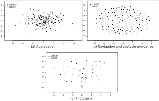
Figure 1: Sammon’s mapping. (a) Aggregation task. Sammon’s mapping of 103 genotypes evolved by odNEAT (black) and 95 genotypes evolved by rtNEAT (gray). (b) Navigation and obstacle avoidance task. Sammon’s mapping of 72 genotypes evolved by odNEAT (black) and 91 genotypes evolved by rtNEAT (gray). (c) Photo-taxis task. Sammon’s mapping of 21 genotypes evolved by odNEAT (black) and 39 genotypes evolved by rtNEAT (gray).

In Figure 1, we show the Sammon’s mapping for the three tasks. The error val-ues are Em = 0.086 for the aggregation task, Em = 0.075 for the navigation and

ob-stacle avoidance task, and Em = 0.082 for the phototaxis task. The low error values

indicate that the distances between genomes are well-preserved by the mapping. In the aggregation task, Sammon’s mapping shows a similar exploration of the search space. odNEAT and rtNEAT explore identical regions in the two-dimensional space, and evolve a comparable number of genomes matching those regions: 103 evolved by odNEAT vs. 95 evolved by rtNEAT. On the other hand, in the navigation task, odNEAT evolves fewer genomes matching the analysed regions of the search space: 72 vs. 91 evolved by rtNEAT. That is, rtNEAT covers more regions of the genotypic search space.

A similar trend is also observed in the phototaxis task, in which rtNEAT evolves 39 genomes vs. 21 evolved by odNEAT.

Since odNEAT relies exclusively on local information, the evolutionary algorithm executing on each robot tends to do a more confined exploration of the search space. In the aggregation task, robots are in close proximity and they therefore continuously ex-change genomes. In such case, the distributed and decentralised dynamics of odNEAT resemble, to some extent, the dynamics of a centralised algorithm. Hence, the explo-ration of the search space performed by odNEAT and rtNEAT is similar, quantitatively and qualitatively. In the other two tasks, because robots tend to be further apart, there is typically more pressure to evolve solutions by using the information available in the population of each individual robot.

5.1.1 Neural Complexity and Generalisation Performance

To the best of our knowledge, there is no general metric for ANN complexity. We use the effective number of parameters in each network, Cfp, which is defined as the sum

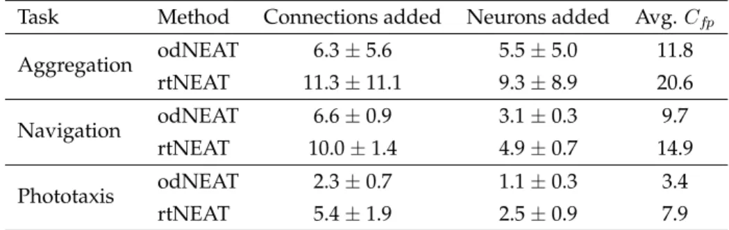
of the number of connections and the number of neurons. This measure of complexity is used in a number of heuristics for the back-propagation algorithm to determine, for instance, a suitable size for the training set (Haykin, 1999). Table 7 lists the complexity reached by each evolutionary method in the final successful solutions. odNEAT’s evo-lutionary dynamics also lead to the synthesis of simpler solutions than in rtNEAT, both in terms of neurons and connections added through evolution. Differences in the neu-ral complexity of evolved solutions are significant in all experimental configurations (ρ < 0.01, Mann-Whitney).

Table 7: Summary of the neural complexity added through evolution from the initial topology by odNEAT and rtNEAT. Connections added and neurons added refer to the avg. ± std. dev. over 30 independent runs for each experimental configuration

Task Method Connections added Neurons added Avg. Cfp

Aggregation odNEAT 6.3 ± 5.6 5.5 ± 5.0 11.8 rtNEAT 11.3 ± 11.1 9.3 ± 8.9 20.6 Navigation odNEAT 6.6 ± 0.9 3.1 ± 0.3 9.7 rtNEAT 10.0 ± 1.4 4.9 ± 0.7 14.9 Phototaxis odNEAT 2.3 ± 0.7 1.1 ± 0.3 3.4 rtNEAT 5.4 ± 1.9 2.5 ± 0.9 7.9

In artificial neural network training, it has been shown that, among a set of solu-tions for a given task, less complex networks tend to have better generalisation per-formance (Schmidhuber, 1997). To compare the generalisation capabilities of odNEAT and rtNEAT, we restart each task 100 times per original evolutionary run. In the task restarts, each robot maintains its controller and further evolution is not allowed. Task restarts are generalisation tests that enable us to assess if robots can continuously oper-ate after several redeployments. The generalisation tests involve both the flexibility to solve the task starting from different initial conditions, and the ability to operate in con-ditions potentially not experienced during the evolutionary phase. A group of robots passes the generalisation test if it continues to solve the task, i.e., if the virtual energy level of any of the robots in the group does not reach zero (see Sections 4.3, 4.4, and 4.5). Each generalisation test has a maximum duration of 100 hours of simulated time.

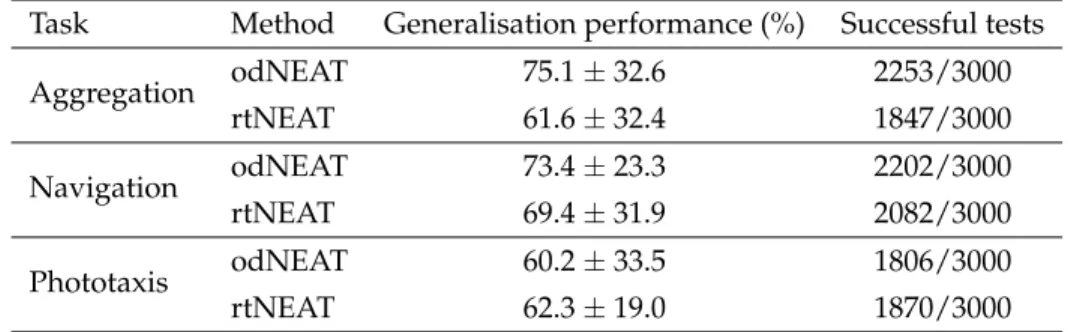
Table 8: Generalisation performance of controllers evolved by odNEAT and rtNEAT in the three tasks. The generalisation performance refers to the avg. ± std. dev. of the success rate for each set of 100 task restarts

Task Method Generalisation performance (%) Successful tests

Aggregation odNEAT 75.1 ± 32.6 2253/3000 rtNEAT 61.6 ± 32.4 1847/3000 Navigation odNEAT 73.4 ± 23.3 2202/3000 rtNEAT 69.4 ± 31.9 2082/3000 Phototaxis odNEAT 60.2 ± 33.5 1806/3000 rtNEAT 62.3 ± 19.0 1870/3000

Table 8 lists the generalisation performance of odNEAT and rtNEAT. In general, odNEAT presents an interesting capacity to generalise and execute in different condi-tions. odNEAT outperforms rtNEAT by approximately 13.5 percentage points in the aggregation task and by 4.0 percentage points in the navigation task, as it successfully solves 406 and 120 tests more, respectively. Differences in successful generalisation tests are statistically significant in the two tasks (ρ = 1.8 · 10−15in the aggregation task, and ρ = 1 · 10−3 in the navigation task, Fisher’s exact test). In the phototaxis task, rtNEAT yields better generalisation performance and successfully solves 64 tests more than odNEAT, which corresponds to approximately 2.1 percentage points. Differences are considerably smaller than in the other two tasks, and are not statistically significant (ρ = 0.095, Fisher’s exact test).

Overall, the analysis performed in this section shows that odNEAT yields perfor-mance levels comparable to those of rtNEAT in terms of the number of evaluations necessary to evolve solutions, and of the task performance of the final controllers. In addition, odNEAT consistently evolves controllers with relatively low complexity and superior generalisation capabilities that can potentially adapt and operate in different deployment scenarios without further evolution.

5.2 Comparing odNEAT and IM-(µ + 1)

In this section, we compare the performance of odNEAT and IM-(µ + 1). Experiments conducted with the IM-(µ + 1) algorithm serve as a means to compare odNEAT with an algorithm with a similar fundamental characteristic: the decentralised online evolution of neural topologies and weights.

Comparison of performance is shown in Table 9. In the aggregation task, odNEAT and IM-(µ + 1) evolve solutions to the task at similar rates. Differences in the number of evaluations between the two algorithms are not statistically significant (ρ ≥ 0.05, Mann-Whitney). In the remaining two tasks, the navigation task and the phototaxis task, odNEAT significantly outperforms IM-(µ + 1) with respect to the num-ber of evaluations (ρ < 0.001, Mann-Whitney). odNEAT requires approximately 54% of the evaluations needed by IM-(µ + 1) in the navigation task, and 45% of the eval-uations in the phototaxis task. Furthermore, odNEAT always evolves controllers that yield significantly higher fitness scores (ρ < 1 · 10−4, Mann-Whitney).

An analysis of the neural complexity of evolved solutions, shown in Table 10, in-dicates that ANNs evolved by odNEAT are also less complex than those evolved by

Table 9: Comparison of the number of evaluations and of the fitness scores of solutions to the task (out of 100) between odNEAT and IM-(µ+1). Values listed are the avg. ± std. dev. over 30 independent runs for each experimental configuration

Task Method Number of evaluations Fitness score

Aggregation odNEAT 103.7 ± 80.9 89.2 ± 4.8 IM-(µ + 1) 100.8 ± 21.9 75.8 ± 10.5 Navigation odNEAT 23.6 ± 19.2 93.0 ± 9.2 IM-(µ + 1) 43.6 ± 10.8 89.5 ± 0.4 Phototaxis odNEAT 40.9 ± 24.1 85.7 ± 6.4 IM-(µ + 1) 91.0 ± 30.6 77.6 ± 9.9

IM-(µ + 1). Both algorithms evolve networks with recurrent and feed-forward con-nections. Differences in Cfp values are statistically significant across the three tasks

(ρ < 0.001, Mann-Whitney). Overall, the IM-(µ + 1) algorithm is biased towards large networks. Since there is no fitness cost in adding new neurons and connections, IM-(µ + 1)consistently generates large neural topologies. The growth is due to the struc-tural mutation operators as: (i) each connection gene has a fixed equal probability of generating a new connection gene in the same genome, and (ii) insertion of new neu-ron genes is based on the duplication and differentiation of a neuneu-ron gene and its in-coming and outgoing connection genes. This form of growth leads to networks that consistently have more connections than neurons added through evolution, as listed in Table 10. Since larger networks have more parameters and need more time to be optimised, either by the adjustment of weighting parameters or the removal of unnec-essary neurons and connections through mutation, the algorithm tends to require more evaluations to find solutions than odNEAT.

Table 10: Summary of the neural complexity added through evolution from the initial topology by odNEAT and IM-(µ + 1). Connections added and neurons added refer to the avg. ± std. dev over 30 independent runs for each experimental configuration. In the IM-(µ + 1) algorithm, the size proportionate addition of new connections and the duplication of neurons, and of their incoming and outgoing connections, lead to networks that consistently have a large number of connections (see text for details)

Task Method Connections added Neurons added Avg. Cfp

Aggregation odNEAT 6.3 ± 5.6 5.5 ± 5.0 11.8 IM-(µ + 1) 23.6 ± 12.2 2.2 ± 0.4 25.8 Navigation odNEAT 6.6 ± 0.9 3.1 ± 0.3 9.7 IM-(µ + 1) 36.7 ± 14.4 2.5 ± 0.6 39.2 Phototaxis odNEAT 2.3 ± 0.7 1.1 ± 0.3 3.4 IM-(µ + 1) 26.0 ± 14.9 1.8 ± 0.5 27.8

In odNEAT, the niching scheme protects topological innovations and also prevents bloating of genomes: species with smaller genomes are maintained in the population as long as their fitness is competitive, and smaller networks are thus not replaced by

larger ones unnecessarily. The successive generation of new candidate controllers leads to a progressive optimisation of existing structure in each robot’s internal population with parsimonious addition of structure.

In odNEAT, the structure of each intermediate solution represents a search space of parameter values that evolution must optimise. The more complex the structure, the higher the number of parameters that must be optimised simultaneously. If the struc-tural complexity can be minimised, the dimensionality of the search spaces explored along the path to a solution is reduced, and evolution can more efficiently optimise the intermediate solutions. Such an approach will generally lead to performance gains in terms of: (i) speed of convergence towards the final solution, i.e., the number of eval-uations, and (ii) the task performance of the intermediate and final solutions evolved. This hypothesis is supported by the results listed in Table 9 and in Table 10, which show that odNEAT evolves less complex networks that always outperform those evolved by IM-(µ + 1) in terms of their ability to solve the task, even when the evaluations neces-sary to evolve a solution are comparable (as in the aggregation task).

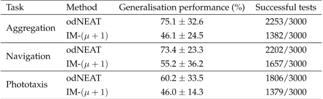
Table 11: Generalisation performance of controllers evolved by odNEAT and IM-(µ+1) in the three tasks. The generalisation performance refers to the avg. ± std. dev. of the success rate for each set of 100 task restarts

Task Method Generalisation performance (%) Successful tests

Aggregation odNEAT 75.1 ± 32.6 2253/3000 IM-(µ + 1) 46.1 ± 24.5 1382/3000 Navigation odNEAT 73.4 ± 23.3 2202/3000 IM-(µ + 1) 55.2 ± 36.2 1657/3000 Phototaxis odNEAT 60.2 ± 33.5 1806/3000 IM-(µ + 1) 46.0 ± 14.3 1379/3000

In the generalisation experiments, we observe that odNEAT evolves controllers that also display a generalisation performance superior to the controllers evolved by (µ + 1), as listed in Table 11. Depending on the task, odNEAT outperforms IM-(µ+1)between approximately 14 percentage points and 29 percentage points, as robots executing odNEAT successfully solve 427 to 871 generalisation tests more. Differences in the number of successful generalisation tests are statistically significant (ρ < 1 · 10−4 in the three tasks, Fisher’s exact test). The results of the generalisation tests are coher-ent with those obtained in Section 5.1.1, which showed that odNEAT evolves neural networks with comparatively high generalisation capabilities. During long-term op-eration in the field, robots may experience environmental conditions not seen during the evolutionary phase. Therefore, producing robust controllers that can adapt to new circumstances without further evolution is advantageous, and has been subject to in-creasing interest (Lehman et al., 2013). Another important aspect in robotic systems is the robustness to failures (Christensen et al., 2009). The following section is devoted to understanding the properties of odNEAT with respect to the algorithm’s ability to adapt to faults in the sensors, and the impact of each algorithmic component on perfor-mance.

6

Assessing odNEAT: Fault Injection Experiments and Ablation Studies

In the previous section, we experimentally compared the performance of odNEAT with the performance of rtNEAT and IM-(µ + 1). In this section, we further assess odNEAT’s robustness and features. We focus on two aspects: (i) odNEAT’s ability to address long-term self-adaptation when there are faults in the robot’s sensors, and (ii) the impact of each algorithmic component on performance.

6.1 Adaptation Performance

The experimental protocol for the fault injection experiments described in this section is defined in coherence with the results of Carlson et al. (2004), which analysed the reliability of 15 mobile robots in terms of physical failures. For small robots operating in the field, such as the models considered in this study, there is an overall frequency of 0.10 failures per hour, and 12% of failures affect the sensors. In their study, the authors do not distinguish between complete failure and partial failure. In our experiments, we assume sensor failures as damaging the sensor completely, and feeding a zero signal into the neural network during subsequent readings.

In the fault injection experiments, we conduct 30 independent runs using a group of 5 robots. We double the duration of each run to 200 hours of simulated time to examine the long-term effects of injected faults. Every hour of simulated time, faults are injected with probability 0.10, in which case one randomly chosen operational physical sensor becomes faulty with probability 0.12. Each robot starts out with the controller evolved in the experiments described in the previous section, but further evolution is allowed. The goal of using evolved controllers is to separate learning to solve the task from learning to overcome sensor faults.

To assess the effects of faults in the sensors, we analyse: (i) the number of con-trollers produced to cope with a given percentage of faulty sensors, and (ii) the op-eration time (age) of the controllers used by the robots during the experiments. The number of controllers produced is an indicator of the difficulty of the evolutionary pro-cess to adapt the behaviour of robots when faults are present. Complementarily, the operation time of controllers relates to the number of faults they can tolerate, thereby indicating the robustness of solutions evolved.

The controllers more robust to faults are those evolved in the aggregation task. On average, robots can sustain faults in approximately 85% of physical sensors, which corresponds to 20 out of 24 physical sensors. After this point, the experiments are terminated because the 200 hours limit is reached. Figure 2 shows the operation time of controllers during the experiments. As more faults are injected, the operation time continues to increase linearly, with a gentle slope, which indicates that new controllers are rarely necessary. In effect, the final controllers operate for more than 100 consecutive hours.

The high robustness to faults in the aggregation task is due to the robot’s behaviour and to the task requirements. Robots form a single group and there is, therefore, con-siderable sensory information available. As long as robots can sense other robots with one or two sensors, faults in the remaining sensors have virtually no effect on per-formance. The high degree of tolerance to faults is due to the exchange of genomes between robots. As described in Section 4.3, the number of genomes received by a given robot is used as an estimation of the number of robots nearby, and is part of the virtual energy level and fitness score computations. Because only the physical sensors of the robots are affected by faults, the virtual energy level and the ”received genomes” sensors function normally and robots continue to solve the task.

0 20 40 60 80 100 120 0 10 20 30 40 50 60 70 80

Avg. operation time (hours)

Avg. percentage of sensor faults per robot Aggregation task -- operation time of controllers

Aggregation

Figure 2: Fault injections during the aggregation task: average operation time (age) of controllers executing at a given time, and subject to a given percentage of faults in the sensors. The operation time increases linearly, with a gentle slope, thereby indicating that new controllers are rarely necessary.

Figure 3 shows the number of controllers produced and the operation time of the controllers in both the navigation and phototaxis tasks. In these two tasks, odNEAT can also adapt to cope with failures in approximately 80% to 85% of the sensors, corre-sponding to a maximum of 14 sensors in the navigation and obstacle avoidance task, and 20 sensors in the phototaxis task. However, contrary to the aggregation task, robots have to evolve new controllers more often to handle the new sensory conditions. In the phototaxis task, with the increasing number of faults, odNEAT progressively tests more controllers as a means to synthesise solutions for the task. As shown in Figure 3(a), when the percentage of faults reaches 50%, each robot had evolved on average 60 new controllers. For a higher percentage of faults, it becomes increasingly more difficult for odNEAT to evolve a suitable solution. When faults affect 75% and 85% of the sensors, the number of controllers evaluated grows to approximately 100 and 160, respectively. This result indicates that robots experience significant difficulties when more than 50% of the sensors are not functional. However, as supported by the approximately stable average operation time of the group for a percentage of faults greater than 50%, shown in Figure 3(b), new controllers are able to sustain a moderate degree of faults in sensors before failing. In terms of neural augmentation, odNEAT continuously adds new topol-ogy in response to the sensor faults. odNEAT adjusts and augments neural topologies from an average of 3.4 parameters added through evolution, for solutions not subject to faults, to approximately 28.2 parameters for solutions subject to faults in 85% of the sensors.

In the integrated navigation and obstacle avoidance task, robots are robust to faults. As shown in Figure 3(a), the initial controller only becomes unable to solve the task when approximately 10% of the sensors fail. From the first fault until 85% of the sensors fail, each robot tested 12.7 new controllers on average. Thus, even though a significant portion of the sensors are faulty, robots only evaluated relatively few new controllers during the entire fault injection experiments. In the synthesis of new con-trollers, odNEAT does not augment neural topologies substantially as the complexity