Carlos Pestana Barros & Nicolas Peypoch
A Comparative Analysis of Productivity Change in Italian and Portuguese Airports
WP 006/2007/DE _________________________________________________________
José Pedro Pontes & Armando J. Garcia Pires
The choice of transport technology in the presence of
exports and FDI
WP 01/2011/DE/UECE _________________________________________________________
Department of Economics
W
ORKINGP
APERSISSN Nº 0874-4548
The choice of transport technology in the
presence of exports and FDI
José Pedro Pontes and Armando J. Garcia Pires
yDecember 6, 2010
Abstract
In a set-up with intermediate production, we analyze how a ship-per’s choice of transport technology, traditionalversus modern, inter-acts with the mode of foreign expansion by an service …rm, export versus foreign direct investment (FDI). In terms of the mode of for-eign expansion by the service …rm, we obtain that: due to trade in intermediate goods, trade and FDI can be complements; the export strategy dominates when the economies of scale at plant level are high and trade costs are low; the FDI strategy is preferable when market size is large and trade costs are intermediate. In what concerns the choice of transport technology by the shipper, we …nd that: the mod-ern technology tends to be implemented in larger markets; economic integration can encourage the adoption of modern technology vis-à-vis the traditional one; the modern technology adoption is more likely for intermediate levels of transport costs. We then have that modern technology adoption usually occurs under the FDI strategy, since both emerge when trade costs are intermediate and market size is large.
Keywords: Transport Technology, Foreign Direct Investment, Trade, Service Sector, Firm Location.
JEL Classi…cation: F23, L12, R30, R40.
Instituto Superior de Economia e Gestão, Technical University of Lisbon, Rua Miguel Lupi 20, 1249-078 Lisboa, Portugal. Tel.: +(351)213925916; Fax +(351)213922808, Email: ppontes@iseg.utl.pt.
yInstitute for Research in Economics and Business Administration (SNF), Breiviksveien
1
Introduction
The literature in international trade and economic geography emphasizes the role of trade costs for economic outcomes, such as trade patterns (Krug-man, 1980), location of industry (Krug(Krug-man, 1991) and multinational activity (Horstmann and Markusen, 1992). In these models, trade costs for example give rise to the well known home market e¤ects, agglomeration e¤ects and the proximity-concentration trade-o¤, respectively1. In addition, the
em-pirical evidence shows that trade costs, transportation technology and the transportation sector play a major role for economic exchange (see amongst others Boylaud and Nicoletti, 2001; Combes and Lafourcade, 2005; Head and Mayer, 2004; Sjostrom, 2004 and Teixeira, 2006). In spite of this important role, transportation has mostly been left in the background of the theoretical analyses. In fact, Paul Samuelson’s (1954) seminal formalization of trade costs, the well known iceberg trade costs, was introduced to avoid precisely dealing directly with the transport sector.
Recently, though, there has been a growing interest on the issues related to transportation. This is the case with for example Mori and Nishikimi (2002), Behrens et al. (2006, 2009), Behrens and Picard (2010) and Taka-hashi (2006). The common topic linking these papers is the relation between transport costs and the location of economic activity. For instance, Mori and Nishikimi (2002) and Behrens et al. (2006) analyze the role of density economies for transport costs. Behrens et al. (2009) and Behrens and Picard (2010) endogenize transport cost rates in a spatial economy. In turn, Taka-hashi (2006) studies the interdependence between the choice of transport technology and economic geography.
In this paper, we follow Takahashi (2006) by focusing on a shipper’s choice of transport technology, modern versus traditional. However, contrary to Takahashi (2006) as well as to the others papers previously mentioned, our main concern is not economic geography but rather to analyze how transport
1The home market e¤ect states that, due to trade costs and increasing returns to scale,
technology is a¤ected by the mode chosen by the service sector to serve the foreign market: export versus foreign direct investment (FDI).
To accomplish this, we develop a model with two players: a monopolist service …rm and a shipper. The economy has two locations: the monopolist headquarters and a foreign (city) market where all the …nal demand is lo-cated. We adopt the export-FDI formalization with intermediate goods by Pontes (2007)2. In particular, the monopolist service …rm produces a …nal
good using an intermediate good as input. Following the literature on FDI (see Carr et al., 2001), the intermediate good can be seen as …rm-speci…c knowledge assets (like blue-prints, patents and tacit knowledge) that need to be pass onto the …nal product. We can think, for example, that the interme-diate good is training given by a …rm’s expert to the …rms’ workers. In turn, the …nal good is a consumption private service good.
The intermediate good can only be produced in the monopolist headquar-ters, but the …nal good can be produced in the monopolist headquarters or in the foreign market. The monopolist has to decide whether to serve the foreign market via exports or FDI. In the export strategy, the …nal good is produced in the monopolist headquarters, while in the FDI strategy the …nal good is produced in the destination market.
In the export case, a …rm’s expert gives training to the …rm’s employees in the headquarters and then they are exported to the foreign market every time the …rm supplies a service there. In the FDI case, instead, a …rm’s expert is exported to the foreign market to give training to the …rm’s workers that are employed in the foreign subsidiary. These employees, in turn, supply the …rm’s service to consumers in the destination market. Both cases are quite common, for instance, with …nancial and consulting …rms.
In turn, the shipper has to choose whether to supply the market with a traditional or a modern technology3. The di¤erence between the two
tech-2Although the focus of the FDI literature has been the manufacturing sector, there is
also a substantial analysis of FDI in the service sector using a very similar framework to the one used for the manufacturing sector (see Markusen and Strand, 2009; Francois and Hoekman, 2010). In fact, Ramasamy and Yeung (2010) show evidence that the standard FDI models (like Horstmann and Markusen, 1992) can also be applied to FDI in the service sector, i.e.: no new theories are necessary to explain the determinants of services FDI (see also Brown and Stern, 2001, Buch and Lipponer, 2007, Moshirian, 2004, Ruckman, 2004). Furthermore, as shown by the World Investment Report 2004, the structure of foreign direct investment (FDI) has shifted towards services. All of the above justi…es our choice of the modeling strategy in this paper.
interna-nologies is that the traditional technology has higher marginal costs and lower …xed costs than the modern technology. In this sense, the main characteristic of the modern technology is that it is subject to increasing returns to scale4. In terms of the mode of foreign expansion by the service …rm, we have that the service …rm only chooses to serve the foreign market (with the ex-port or the FDI strategy) at relatively low transex-port costs. In addition, as in Horstmann and Markusen (1992), the usual trade-o¤ between concen-tration and proximity arises in the decision of the monopolist service …rm. In particular, while the export strategy is preferred when the economies of scale at the plant level are high and transport costs are low (concentration), the FDI strategy is favored when market size is large and trade costs are intermediate (proximity). However, contrary to Horstmann and Markusen (1992), but in line with Pontes (2007), due to intermediate consumption, FDI does not necessarily eliminate exports. In other words, FDI and exports need not be substitutes, since under FDI, international trade continues to arise due to the exports of intermediate goods (i.e.: FDI and exports can be complements). This result has two advantages: …rst, our model mirrors bet-ter the real world than standard horizontal FDI models such as Horstmann and Markusen (1992), since the data show that FDI and exports tend to be complements (see Markusen, 2002); second the demand for transportation under FDI is positive (and not zero as is the case when FDI and exports are substitutes)5.
tional level, i.e.: inter-city transport infrastructure but not intra-city. Larch (2007) show evidence of the growing importance of the multinationalization of the transport sector. For the study of intra-city (urban) transport infrastructure, see Zenou (2000, 2011).
4The metaphor modernversus traditional does not need to be read literally. We can
instead think of an established transport technology (which can be hi-tech or not) and a new technology, where for the former the …xed costs have already been incurred, but the same is not the case for the latter.
5Horizontal FDI occurs when production takes place in the …nal destination. The other
The latter feature is central in a set-up like ours that aims to analyze the choice of transport technology. In fact, if FDI and trade are substitutes, the demand for transportation when the monopolist chooses the FDI strategy would be zero, given that there is no trade. As a consequence, under the FDI equilibrium, the shipper would never adopt the modern technology, since it could not pay for the modern technology’s …xed cost. On the contrary, if FDI and trade are complements, even under the FDI regime the shipper can choose between the modern and the traditional technology, since interna-tional trade in intermediate production creates a demand for transportation. Accordingly, it might then be possible for the shipper to pay for the modern technology’s …xed cost.
In what concerns the shipper’s choice of transport technology, we obtain three main results. First, the modern technology tends to be implemented in larger markets. This is so, given that a larger market size reduces the …xed costs per capita of the modern technology, making its adoption more attractive relatively to the traditional one. Second, economic integration may encourage the adoption of the modern technology vis-à-vis the tradi-tional one. The ratradi-tionale for this is that closer economic integration increases trade, thereby allowing the shipper to pay for the higher …xed costs of the modern technology. Third, the relation between transport costs and mod-ern technology adoption is non-monotonic. More precisely, the adoption of modern technology takes place for intermediate levels of transport costs. To understand this, note that for high transport costs the demand for trans-portation is low, and for low transport costs the returns from transtrans-portation are low (although demand is high).
We then observe that the shipper’s choice of transport technology is di-rectly related to the service …rm’s mode of foreign expansion. First, the modern technology will only be adopted if the service …rm enters the foreign market (with either the export or FDI strategies), i.e.: when trade costs are not extremely high. The reason for this is straightforward: only when trade exchanges emerge in the economy is it worthy for the shipper to incur the …xed costs of the modern transport technology. Second, the modern tech-nology is more likely to be adopted under FDI. The basis for this outcome is that both the FDI strategy and the modern technology are more pro…table in larger markets and for intermediate levels of trade costs.
we introduce the base model. In section 4, we study the choice of foreign expansion by the monopolist service …rm. In section 5, we analyze the choice of transport technology by the shipper. In section 6, we conclude.
2
Case Study: The High-Speed Rail
To our knowledge there is very little empirical evidence on the adoption of modern transport technologies. In order to …nd support for our theoretical results we look, instead, to the pattern of development of the HSR in some countries and regions of the world6. We base our analysis on a review on the following HSR literature: Campos et al. (2007); Freemark (2009); Hood (2006); Perren (1998), The Economist (2010) and The World Bank Railway Database.
The HSR is a modern train technology, and as the name says the HSR operates signi…cantly faster than conventional trains7. The …rst HSR was
Japan’s Shinkansen, also known as the "bullet train", which started o¢cially operating in 1964 between Tokyo and Osaka. In the 1970’s, France began to develop the French version of the bullet train, the TGV (Train à Grande Vitesse, literally high-speed rail). In 1981, France opened the …rst HSR connection between Paris and Lyon. Since then, France’s HSR network has been expanded to connect cities not only across France but also in adjacent countries, in particular Belgium, Netherlands and England. In addition, the European Union (EU) is currently …nancing a trans-European network of high-speed rail that will link France’s TGV to other European countries, such as Italy, Spain, Germany, Poland, Austria, Switzerland and Portugal8.
In the rest of this section, we will focus our analysis in four countries (Japan,
6This exercise, however, cannot enlighten us on how the choice of transport technology
interacts in the real world with the mode of foreign expansion by …rms. In our view, and given the shortage of studies on the topic, this is an interesting issue for future research.
7A train connection is considered to be high speed if it runs 200 km/h (120 mph) for
upgraded tracks or 250 km/h (160 mph) or faster for new tracks. HSR is mostly used for passenger transportation. However, in some cases is also used for goods transportation, especially light goods, but also in some cases for bulk transportation (for instances the French post uses HSR to transport mail).
8Even more ambitious is China’s plan for 50 000 kilometers (31 000 miles) of HSR lines
France, Spain and Italy) and one region (Europe) with established HSR networks. Our main conclusions do not change if we consider other countries with HSR.
Anticipating the results from our small case study, we observe three pat-terns related to the HSR adoption. First, the target areas for HSR connec-tions are pairs of major cities. Second, economic integration can promote the adoption of the HSR across countries. Third, the HSR tends to be built between cities that are not too far apart or too close together9. As we will
see in the next sections, this is exactly what our model …nds. Next we seek to provide evidence that supports our claims.
We start by analyzing the argument on population and HSR links. In Japan, after the construction of the line between Tokyo and Osaka in 1964 (the …rst and third cities in Japan, respectively)10, Osaka-Hakata (Fukuoka)
followed in 1972, Tokyo-Hachinohe and ¯Omiya-Niigata in 1982,
Takasaki-Nagano in 1997 and Shin Yatsushiro-Kagoshima Ch¯u¯o in 2004. Fukuoka
is the largest Japanese city west of Osaka. Hachinohe is the largest city in the eastern Aomori prefecture. ¯Omiya is one of the hub stations in the Greater Tokyo Area. Niigata has a population of approximately 800 000 (but the population of the Niigata prefecture is around 2.4 million) and Kagoshima is located at the southwestern tip of the island of Japan with a population of about 600 000. Takasaki, Nagano and Yatsushiro are smaller cities. However, Takasaki functions as a regional transportation hub for Japan’s Shinkansen. In turn, Nagano and Yatsushiro are intermediate stops on the planned extension of the Osaka-Fukuoka line to the south and west regions of Japan, respectively.
As already mentioned, in France the link between Paris and Lyon (…rst and second regional agglomerations in France) was completed in 1981. This was followed by Paris-Tours-Le Mans in 1990, Lyon-Valence in 1992, Valence-Marseille in 2001 and Paris-Strasbourg in 2007. While Tours and Le Mans are not very large cities, they are part of the commuter belt of Paris11. In turn,
the Paris-Valence connection was developed as a step on the way to Marseille (the third largest agglomeration in France). Strasbourg is only the seventh largest city of France but it hosts several important European institutions
9In our model, the rate of transportation is proxied by distance.
10Yokohama is the second largest city in Japan but is part of the Greater Tokyo Area.
11In addition, the Paris-Tours-Le Mans link is planned to be extended to Bordeaux (the
such as the Council of Europe, the Eurocorps, the European Parliament and the European Union Ombudsman.
In Spain the main existing HSR connections are Madrid-Seville, opened in 1992; Madrid-Valladolid in 2007 and Madrid-Barcelona in 2008. Madrid, Seville, and Barcelona are respectively the …rst, fourth and second largest cities in Spain. Valladolid is not a very large city (it has a population of just 320 000) but it is planned to be part of the HSR connection to the Basque country (third largest region in Spain after Madrid and Catalonia) and to Portugal12.
In turn, the aim of the Italian HSR network is two-fold: to connect Naples-Rome-Florence-Bologna-Milan and Turin-Milan-Venice. The follow-ing segments of these two lines are already in operation: Florence-Rome opened in 1991, Rome-Naples in 2005, Milan-Bologna in 2008, Turin-Milan and Bologna-Florence in 2009 (Milan-Venice is still under construction). Mi-lan, Rome, Naples and Turin are the …rst, second, third and fourth largest metropolitan areas in Italy, respectively. Florence, Venice and Bologna are only in the second tier of the largest cities in Italy. However, Florence and Venice are amongst the world’s top tourist cities and Bologna is a hub in Italy’s train network. From the above, we can conclude that the countries analyzed have prioritized HSR connections between larger cities.
We now turn to the second point related to economic integration. Eco-nomic integration lowers the costs of exchanging goods across borders. It is a well established fact that transport costs are higher at the international than at the national level. For example, if two regions are equally distant from each other, the trade costs tend to be higher when the two regions belong to two di¤erent countries than when they are part of the same country (see Anderson and van Wincoop, 2003, 2004).
It can be easily noted that of all the regions in the world with HSR, only in Europe were international connections established. As already mentioned, the center of the trans-European HSR network has been France. The …rst international HSR link in Europe was opened in 1993 between Paris and Brussels and was shortly afterwards extended to Amsterdam13. In 1997 the
high speed line between Paris and London began operation with trains
pass-12A HSR connection to Valencia, Spain’s third largest city, is also under construction.
13Brussels is the de factocapital city of the EU and the largest urban area in Belgium
ing undersea through the famous purpose built Channel Tunnel14. Shortly
afterwards, Brussels was linked with Cologne in Germany15. Currently,
con-nections of the France’s HSR system to Spain (Madrid and Barcelona), Italy (Turin and Milan), Switzerland (Zurich), and Germany (Frankfurt) are un-der construction. In addition, other international links are being planned: Netherlands with Germany, Austria with Germany, Italy with Germany, Slovenia with Switzerland, Sweden with Denmark and Germany, Poland with Germany, and Spain with Portugal.
Given that Europe constitutes the most developed experience of regional economic integration (via the EU) in the world, this seems to con…rm that the adoption of modern technologies in transportation is facilitated by closer economic integration.
We close by discussing the third argument on distance and HSR. Start by noticing that if we compare HSR with other modes of transportation, like air and road travel, we have the following. The HSR is less competitive than air travel for longer distances (like Paris-Moscow), and more competitive for journeys of up to two to three hours (250-900 kilometers or 150-550 miles)16.
In turn, the HSR is more competitive than road transportation for longer distances, while the latter compares favorably for shorter distances, especially when there is little congestion (i.e.: when road transportation occurs between locations with a small market size).
In fact, and as we have mentioned, HSR tends to link cities within the same country, where distances are usually smaller than between cities in di¤erent countries. Also, when international connections were established (which, as we have seen, is only the case in Europe), the …rst lines opened were amongst cities located at intermediate distance from each other. For example, there is a HSR between Paris and Brussels situated 261 kilometers apart (162 miles) but not between Paris and Berlin at a distance of 876 kilometers (544 miles), although Berlin is more populated than Brussels. In this sense, we have that HSR networks tend to connect cities located at mid
14London is UK’s largest and most populous metropolitan area and the largest urban
zone in the European Union with about 14 million inhabitants.
15Cologne is Germany’s fourth-largest city, and one of the major European metropolitan
areas with around 10 million inhabitants.
16The reason for this is that not only are the formalities with checking-in and security less
distance from each other, but not cities that are either too close or too far apart17.
3
The Model
The model has two players: a monopolist service …rm (henceforth player I) and a shipper (player S). The economy consists of two locations: the monopolist headquarters and the foreign market withn consumers where all …nal demand is located. The monopolist has to choose whether or not to supply the foreign market, and if it does, the monopolist has to decide the mode of entry: by means of export or FDI. In turn, the shipper has to select which transport technology to adopt: traditional or modern. Let f(p) be a demand function (p is the delivered price), which we assume to be:
Continuous Decreasing
Revenue function pf(p) is strictly concave.
Remark 1 Together these assumptions imply that dpdc > 0 for all values of c, where c stands for a constant marginal cost and p is a pro…t maximizing price.
To produce the …nal good, the monopolist needs an intermediate product (training), which has to be produced in-house in the monopolist headquar-ters. In turn, the …nal good (service) can either be produced in the mo-nopolist’s headquarters or in a plant in the foreign market. In case of the former, we say that the monopolist follows the export strategy, since the …nal
17The adoption of the railway in the nineteenth century apparently had a similar
good is exported to the foreign market. In the latter case, the monopolist pursues the FDI strategy, given that a production plant is established in the destination market. In this sense, in the FDI strategy the …nal good is sold directly to consumers, but the intermediate good needs to be exported in order to be incorporated in the …nal good. We further assume that the price of the intermediate good is w and that …rm I uses 2 [0;1] units of the intermediate good to produce one unit of the consumer good.
As discussed in the introduction, we can think of the intermediate good as …rm-speci…c knowledge assets (like blue-prints, patents and tacit knowledge) that are required to be transmitted to the …rm’s employees in order for them to be able to supply the …rm’s service to …nal consumers. We then have that in the export strategy a …rm’s expert gives training to the …rms’ employees in the headquarters. Subsequently, when a …rm sells a service, the trained employees are exported to the foreign market to supply the service. In the FDI strategy, instead, a …rm’s expert is exported to the foreign market in order to give training to the …rm’s employees in the foreign subsidiary. These employees, in turn, supply the service to consumers in the foreign market.
Export has over FDI the advantage of lower …xed costs. The expert that gives training to the workers in the foreign city has to set up a local plant thus incurring in costs related with indivisible assets that we express by the …xed cost G. By contrast, FDI entails lower transport costs than Export: if m denotes the unit variable cost of the …nal service good, the transport cost of the intermediate good will be m < m. This is so because the intermediate good is a piece of information (as in Carr et al. 2001), so that it has the nature of a public good inside the …rm. A single expert can jointly train several workers in the foreign city. Thus, under FDI the travel of the expert substitutes for the multiple travels the trainees would have to accomplish were the training activity occur in the home city.
FDI models assumes that FDI and trade are substitutes (Markusen, 2002). With FDI and trade as potential complements, our set-up gains not only in realism, but it also becomes more suitable for analyzing the topic we propose to study. In fact, and as we have just seen, if FDI and trade are substitutes it means that there is no trade under FDI, i.e.: the demand for transportation would be zero with FDI. In this sense, the FDI decision would become redundant for the choice of transport technology, i.e.: only with exports would the shipper evaluate the alternative transport technologies
(traditional versus modern). On the other hand, with FDI and trade as
complements it means that there is trade under FDI (in our case, this is due to trade in intermediate goods), i.e.: the demand for transportation is positive with both export and FDI. Therefore, even when the service …rm chooses FDI (and not only with exports), the shipper can ponder about what is the pro…t maximizing transport technology to serve the foreign market.
The game has two stages. In the …rst stage, the monopolist chooses the mode of entry (exit, export or multinational) and the shipper decides on transport technology (traditional or modern). In the second stage, the monopolist sets a delivered price p.
We need to be more precise about the decision in the …rst stage. In what concerns the monopolist, we have that it chooses between three alternative ways to supply the foreign market:
"0": Exit, I refrains from supplying the foreign market. "E": Export, I supplies the foreign market through exports. "D": FDI, I supplies the foreign market through a local plant.
As standard in the FDI literature (see Horstmann and Markusen, 1992), we assume that it is more costly to operate a plant away from the headquar-ters than close to it. This can be due to higher communication, transport or knowledge transfer costs, which are usually higher when the plant is far away from the headquarters. Without loss of generality, we then assume that the plant-speci…c …xed costs are zero in the case of exports and equal toGunder the FDI strategy.
The choice between the export and the FDI strategy can then be modeled as in Pontes (2007):
I 0 = 0
I
I
D(p; G; m) = n(p w m)f(p) G, (1)
Applying a positive linear transformation that consists in dividing the
payo¤s by 1
n, we obtain the following:
I 0 = 0
I
E(p; m) = (p w m)f(p)
I D(p; G
c; m) = (p w m)f(p) Gc, (2)
whereGc = G
n are per capita plant-speci…c …xed costs.
In turn, the shipper chooses between two transport technologies:
A traditional technology "T" with positive variable costs and zero …xed costs, whose pro…t function is:
S
T = (t m)Q, (3)
wheret transport rate and Q demand for transport.
A modern technology "M" with zero variable costs and a positive …xed sunk cost F, whose pro…t function is18:
S
M =tQ F. (4)
In order to simplify, we assume that t = m (t is a parameter for both players) because the monopolist …rm can always carry the product itself "on foot" using the traditional technology.
Applying again a positive linear transformation that consists in dividing the payo¤s by n1, we have that the pro…t functions for the traditional and the modern technology equal (and since t =m):
S T = 0
S
M =mQ
c Fc, (5)
18In this sense, we can think of the modern technology as the HSR and the traditional
Monopolist
Exit (0) Export (E) FDI (D)
Shipper Traditional 0,0 0,f(p)(p-αw-m) 0,f(p)(p-α(w-m))-GC
Modern -FC,0 f(p)m-FC, f(p)(p-αw-m) αf(p)m-FC, f(p)(p-α(w-m))-GC
Figure 1: Payo¤ matrix
where Qc = Qn are the per capita demand for transport and Fc = F n are
the per capita …xed costs of the modern technology.
Note then that demand for transportation under export and FDI isQE =
f(p) and QD = f(p), respectively. This, together with the above, implies
that the …rst stage payo¤ matrix is as in …gure 1.
We can now analyze in more detail the choices of the monopolist and the shipper. We start with the monopolist and then move to the shipper.
4
Choice of the Mode of Foreign Expansion
From equations 1 and 2, we can see that the decision by the monopolist is independent from the one by the shipper19. It is assumed that for each value
of m, the …rm selects a pro…t-maximizing price. Then, in both cases E and D, this price is an increasing function of m. We de…ne:
I
E(m) = maxp I
E(p; m)
I D(G
c; m
) =max
p I
D(p; m; G c
). (6)
To analyze the decision between the strategies E and 0, note …rst that
I
E(m)is a continuous function and that:
19In the last section paper we discuss the consequence of relaxing this restriction in our
I
E(0)>0
lim
m!1
I
E(m)<0. (7)
Furthermore, function I
E(m)is decreasing, since using the envelope
the-orem:
d I E
dm =
@ I E
@m = f(p)<0. (8)
Hence, there is a unique thresholdm, such that (see …gure 2):~
I
E(m)R0 i¤ mQm.~ (9)
In turn, the choice between strategiesDand 0can be analyzed by means of the implicit function:
I D(G
c; m
) = 0. (10)
Using the implicit function theorem on I
D(m; Gc), we …nd that
every-where there is a continuous functionGc(m)whose …rst and second derivatives
are:
dGc
dm = f(p)<0
d2Gc
dm2 = f
0
(p)dp
dm >0. (11)
The Gc(m) function is then decreasing and convex (see …gure 2). It
can be concluded that Gc(0) is positive and …nite and lim m!1
I
D(Gc; m) <0,
so that Gc(m) intercepts the m axis. Moreover the value G~c is such that I
D G~c;m~ = 0is positive, since the operating pro…t of strategyDis positive
for m= ~m. We then have:
f(p) (p w m~)> IE( ~m) = 0. (12)
H(Gc; m) = 0, IE(m) I D(G
c; m
) = 0. (13)
Using again the implicit function theorem, we have that there is a con-tinuous function Gc(m)that passes through the origin in space (Gc; m) and through the point G~c;m~ . This function has the following …rst and second
derivatives:
dGc
dm =
Hm
HG
= (1 )f(p)>0
d2Gc
dm2 = (1 )f
0
(p)dp
dm <0. (14)
Gc(m) is thus increasing and concave (see …gure 2). Pulling together the results obtained so far, we can plot the E, D and 0 regions in the space
(Gc; m). The di¤erent areas in …gure 2 indicate where each strategy of serving
the consumers in the foreign market is more pro…table for the monopolist …rm20.
From …gure 2, we can see that like in Horstmann and Markusen (1992) the proximity-concentration also holds. In this sense, the export strategy is preferred for high Gc (high economies of scale at the plant level and small
market size) and low m (low transport costs). The multinational strategy, in turn, is favored for smallGc (low economies of scale at the plant level and large market size) and mid-high m (medium-high transport costs). In the next section, we will analyze the shipper’s choice of transport technology and how this decision interacts with the mode of foreign expansion by the service …rm.
5
Choice of Transport Technology
The decision of the shipper depends upon the monopolist’s choice of foreign expansion. In particular, as can be seen from …gure 1, the decision of the shipper is:
If Exit (0): Traditional (T)
20The thick dashed curve depicts the monopolist service …rm’s decision between the
strategies E-0. In turn, the thick solid curve for m < m~ and m > m~ represents the
Export (E)
FDI (D)
No- entry (0)
No- entry (0) c
G
m
FDI (D) Export
(E) c
G~
m~
Figure 2: Location of the monopolist in space (Gc; m)
If Export (E): Modern (M) i¤ f(p)m Fc 0; Traditional (T) i¤
f(p)m Fc <0
If FDI (D): Modern (M) i¤ f(p)m Fc 0; Traditional (T) i¤
f(p)m Fc <0
It is evident that the best reply by the shipper to exit (0) is the traditional (T) transport technology, since the demand for transport services is then zero. Therefore, the modern technology (M) can only be chosen in equilibrium if the monopolist decides to supply the foreign market through exports (E) or FDI (D).
De…ne QcD per capita transport demand under FDI (with trade in
intermediate goods) and Qc
E per capita transport demand under Export.
It then follows:
QcE = f(p( w+m))
QcD = f(p( (w+m))). (15)
Let Qc =Qc
Without loss of generality assume thatw= 0. The relation betweenLE(m) =
f(p(m))m and LD(m) = f(p( m)) m is therefore undetermined.
In the export case, the following condition ensures both that the modern technology is feasible for the shipper and that it is preferred to the traditional one:
f(p(m))m Fc 0 (16)
or:
Fc LE(m) =f(p(m))m. (17)
Function LE(m) is de…ned in [0;m~] for high enough values of Gc, so
that the monopolist chooses to supply the foreign market through exports. According to the de…nition ofm~, functionLE(m)has the following properties:
1. LE(0) = 0
2. LE(m) is increasing in the neighborhood of0 since:
signdLE(m)
dm =sign
2
4f(p(m))
(+)
+mf0(p(m)) dp
dm
( )
3
5, (18)
whose sign is ambiguous. However, since the derivative is continuous by assumption, and dLE
dm jm=0= 0, it follows that it is also positive for m in the
neighborhood of 0.
3. LE( ~m) =f(p( ~m)) ~m =f(p( ~m))p( ~m) = ~FEc >0.
In the FDI case, the condition for the adoption of the modern technology is:
f(p( m))m Fc 0 (19)
or:
Fc LD(m) = f(p( m))m. (20)
The functionLD(m) has the following properties:
1. LD(0) = 0
signdLD(m)
dm =sign
2
6
4f(p( m))
(+)
+ mf0(p) dp
d( m)
( )
3
7
5, (21)
whose sign is ambiguous. However, since the derivative is continuous by assumption, and dLD
dm jm=0>0, it follows that it is also positive for m in the
neighborhood of 0.
3. LD( ~m) =f(p( ~m)) ( ~m) = ~FDc >0, sincef(p( ~m))>0.
4. LD(m)is decreasing for arbitrary high values ofm. This is so because:
(i) f(p( m)) ! 0 when m ! 1 (note that m ! 1 when m ! 1 and
p( m) increases without bound with m); (ii) mf0(p)d(dpm) ! 1 when m ! 1, once the assumptions on the demand function ensure thatf0(p)<0
and d(dpm) >0 for all p.
The fact thatLD(m)is eventually decreasing with the transport rate (m)
in the FDI region, together with the observation that the rise ofmdetermines a switch from FDI to exit, makes the adoption of the modern technology less likely for high variable transport rates. This means that the increase of the variable transport rate (proxied by distance) reduces the demand for transport services, thus preventing the modern transport technology to break even. In this sense, the adoption of modern transport technology tends to occur in the vicinity of m~.
We then need to analyze the relations between:
~
FEc = LE( ~m) = f(p( ~m)) ~m=f(p( ~m))p( ~m) ~
FDc = LD( ~m) = f(p( ~m)) ( ~m)< f(p( ~m))p( ~m) ~
Gc = (p( ~m) m~)f(p( ~m)). (22)
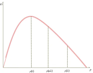
Start by looking at the total revenue function,pf(p). The total revenue function is concave and has a unique maximum (see …gure 3). Then we clearly see that the relations between F~Ec, F~Dc, and G~c are undetermined.
We therefore need to examine how the equilibrium of the game changes for di¤erent relations between F~c
( )0
p )
(p p f
p
( )m
pα~ p( )m~
Figure 3: Total revenue function
(1)G~c > F~Ec >F~Dc (2)G~c > F~Dc >F~Ec (3)F~Ec > G~c >F~Dc (4)F~Ec > F~Dc >G~c (5)F~Dc > G~c >F~Ec
(6)F~Dc > F~Ec >G~c. (23)
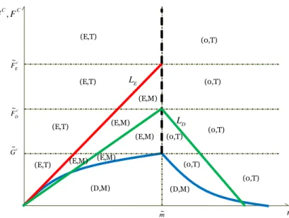
Figures 4 to 9 show the equilibrium choice of transport technology for the cases in equation 23 as a function of the monopolist’s mode of foreign expansion (exit, export, FDI)21. From …gures 4 to 9, we can observe three
patterns related to the choice of transport technology by the shipper alone
21In …gures 4 to 9,G=F, i.e.: the …xed costs of the monopolist equal the …xed costs of the modern technology. We make this assumption in order to be able to make a graphical representation of the equilibrium of the game. However, note that even so G~c
, F~c
E and
~ Fc
D di¤er. The LE(m) andLM(m) curves are signed with their respective names. The LE(m)curve, though, is easy to identify since it is truncated form >m~, i.e.: form >m~
and two patterns that concern how the choice of the shipper interacts with the decision on the mode of foreign expansion by the service …rm. Start with the former. First, we have that as market size increases (lowGc and lowFc)
the modern technology is promoted. Accordingly, larger market size allows the shipper to explore the economies of scale of the modern technology.
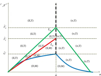
Furthermore, the relation between market size and modern technology adoption tends to be monotonic. There is, however, one exception: case (3), whereF~Ec >G~c >F~Dc. When this occurs as market size increases, the modern technology is only monotonically adopted in relation to the same mode of foreign expansion, but not when export gives place to FDI, i.e.: (E; T) ! (E; M)!(D; T)!(D; M). Note however, that the non-monotonic relation only arises for intermediate levels of m (lower than m~, but in its vicinity), for lower and higher levels of m the relation is always monotonic, as it takes place in the other cases (case (1), (2), (4), (5) and (6)). The reason for the non monotonicity is that in case (3) there is a large di¤erence between the level of …xed costs that leads to the adoption of the modern technology under exports and under FDI, i.e.: F~Ec >> F~Dc. This can occur for example when trade in intermediate goods is small under FDI, and therefore the level of …xed costs that makes the modern technology pro…table under FDI is also low.
Second, decreasing transport costs (m) can encourage the adoption of the modern technology. The rationale for this is that as trade costs decrease, the demand for transportation increases, making the modern technology more pro…table than the traditional one. The previous result indicates that fur-ther economic integration creates a good environment for the introduction of modern transportation technologies.
Third, the relation between transport costs (as proxied by distance) and the modern technology adoption is non-monotonic. In particular, as dis-cussed above, the modern technology tends to be chosen by the shipper in the vicinity of m~ (i.e.: for intermediate levels of transport costs and in the limits of the export strategy). For either high or low transport costs the traditional technology is preferred. The reason for this is that with high
high values of m. In the …gures below, we have depicted thatLD(m)starts to decrease
for m = ~m. However, the results are not changed qualitatively if LD(m) is decreasing
only for m > m~. As in …gure 2, the thick dashed curve depicts the monopolist service
…rm’s decision between the strategies E-0. The thick solid curves form <m~ andm >m~
represents the monopolist service …rm’s decision between the strategies D-E and D-0,
variable transport costs, demand for transportation is very low, and there-fore the modern technology is not appealing for the shipper since economies of scale in transportation are also low. In turn, for low trade costs (i.e.: over short distance), while the demand for transportation is high, the returns from transportation are so low that the shipper …nds it di¢cult to pay the …xed costs of the modern technology.
In terms of the relation between the choice of the service …rm and of the shipper, we have the following. First, and as already mentioned above, if the service …rm does not enter the market, then it is also not pro…table for the shipper to adopt the modern technology. This is so, since in this scenario, there are no trade exchanges.
Second, the modern technology tends to arise together with the FDI strategy. The reason for this is that both the modern technology and the FDI strategy are more likely to emerge when market size is large and trade costs intermediate. However, the modern transport technology can also oc-cur jointly with the export strategy. This is only the case, though, when
~
FEc >G~c (…gures 6, 7 and 9), i.e.: when the modern technology is pro…table for relatively high levels of …xed costs and the export strategy is pro…table for relatively low levels of plant-speci…c …xed costs.
Given that the export strategy is relatively more intensive in transporta-tion (since 2 [0;1]), it might seem a counter intuitive outcome that the modern transport technology is more likely to arise when the service …rm chooses the FDI strategy than with the export strategy (although, as we have just seen the modern technology can also arises together with the ex-port technology, see …gure 6, 7 and 9). In other words, we would expect à priori that the modern technology would potentially be more attractive under the export strategy than under the FDI strategy. However, this is not the case, because in the end what is more important for the shipper’s decision is not only the intensity of transportation under a given mode of foreign expansion by the service …rm, but also the pro…tability of a given transport technology as determined by market size. And as we have just seen, it comes out that when market size is large the decisions of the ship-per and of the service …rm converge for the modern technology and the FDI strategy, respectively.
(0,T) (E,T)
(D,M) C
C
F G ,
m
(D,M) (E,T)
(E,T)
(E,T)
(D,T)
(D,T)
(D,T)
(D,T)
(D,T)
(D,T)
(D,T) (0,T)
(0,T)
(0,T) E
L
D
L
m~
c E F~
c
G~
c D F~
Figure 4: Transport technology in space ((Gc; Fc); m): (1) G~c >F~Ec >F~Dc
the interactions between the decisions of the shipper and the service …rm, since in our case study we do not compare FDI and export data with the introduction of the HSR. For analyzing the relations between the mode of foreign expansion by …rms and the adoption of modern transport technologies by shippers, we would need a fully ‡edged econometric model with data on exports and FDI. In our opinion this is an interesting topic for future empirical research.
6
Discussion
In a set-up with intermediate production, we have analyzed how a shipper’s choice of transport technology (traditional versus modern) is a¤ected by the mode of foreign expansion by a service …rm (export versus foreign direct investment).
m (D,M) (0,T) (E,T) (E,T) (D,M) (D,T) C C F G , (E,T) (E,T) (D,T) (D,T) (D,M) (D,M) (D,M) (0,T) (0,T) (0,T) (D,T) E L D L m~ c E F~ c G~ c D F~
Figure 5: Transport technology in space ((Gc; Fc); m): (2) G~c >F~c D >F~Ec
m (D,T) (0,T) (E,T) (E,T) (D,M) C C F G , (E,M) (E,T) (E,T) (D,M) (D,T) (D,T) (D,T) (D,T) (0,T) (0,T) (0,T) E L D L m~ c E F~ c G~ c D F~
Figure 6: Transport technology in space ((Gc; Fc); m): (3) F~c
m (E,M) (0,T) (E,T) (E,M) (D,M) C C F G , (0,T) (0,T) (E,M) (E,T) (E,T) (E,T) (E,M) (E,M) (D,M) (0,T) (0,T) (0,T) E L D L m~ c E F~ c G~ c D F~
Figure 7: Transport technology in space ((Gc; Fc); m): (4) F~c
E >F~Dc >G~c
m (0,T) (E,T) (D,M) (E,T) (D,M) (0,T) C C F G , (E,T) (E,T) (D,M) (D,M) (D,M) (0,T) (0,T) (0,T) (0,T) (0,T) (D,T) (E,T) (E,T) (D,T) (D,T) E L D L m~ c E F~ c G~ c D F~
m
(0,T) (E,T)
(E,M)
(D,M) (E,T)
(0,T)
(0,T) C
C
F G ,
(E,T)
(E,T) (E,M)
(E,T)
(E,T)
(E,T)
(0,T)
(0,T)
(0,T) (0,T)
(D,M) E
L
D
L
m~ c
E F~
c
G~ c D F~
Figure 9: Transport technology in space ((Gc; Fc); m): (6) F~c
D >F~Ec >G~c
FDI and trade as substitutes).
In what relates to the shipper’s choice of transport technology, we obtain the following. First, the modern technology tends to be implemented in larger markets, since the shipper can explore larger economies of scale in the modern technology. Second, economic integration can help to promote the adoption of the modern technology, given that it increases international trade and therefore transport demand. Third, the adoption of modern technology tends to arise for intermediate levels of variable transport costs (as proxied by distance), since for high transport costs the demand for transportation is low and for low transport costs the returns from transportation are small.
The above results seem to …t well with the adoption of modern trans-port technologies, such as the HSR. In fact, we have observed that the HSR tends to connect large cities that are not too far apart or too close together. Furthermore, the European experience of closer economic integration has triggered the adoption of HSR across European borders.
Second, the adoption of modern technology tends to take place together with the FDI strategy, once they both emerge for intermediate levels of trade costs and when market size is large.
Given that we have not provided evidence to support the two previous …ndings, future empirical research could analyze the relation between the adoption of modern transport technologies (such as the HSR) and the dom-inant mode of foreign entry by …rms, such as export and FDI.
In addition, future work could extend our model to introduce competition in the service sector, competition in the transport sector, and endogenize the rate of transportation. Competition in the service sector in principle will not change our main results since the proximity-concentration trade-o¤ still holds in duopoly and oligopoly market structures (see Markusen, 2002). Competition in the service sector, in turn, would only be relevant with imperfect competition between transporting …rms (since with perfect competition marginal cost pricing would hold). With imperfect competition in the transport sector, we could also endogenize the rate of transportation. In this way, the mode of foreign expansion in the service sector and the choice of transport technology in the transport sector would be mutually dependent.
References
[1] Anderson, J. and van Wincoop, E. (2003), Gravity with gravitas: A solution to the border puzzle, American Economic Review, 93, 170-192.
[2] Anderson, J. and van Wincoop, E. (2004), Trade costs, Journal of Eco-nomic Literature, 42, 691-751.
[3] Behrens, K., Gaigné, C., Ottaviano, G. and Thisse, J.-F. (2006), How density economies in transportation link the internal geography of trad-ing partners, Journal of Urban Economics, 60, 248-263.
[4] Behrens, K., Gaigné, C. and Thisse, J.-F. (2009), Industry location and welfare when transport costs are endogenous, Journal of Urban Economics, 65, 195-208.
[6] Boylaud, O. and Nicoletti, G. (2001), Regulatory reform in road freight, OECD Economic Studies, 32, 229-251.
[7] Brown, D. and Stern, R. (2001), Measurement and modeling of the economic e¤ects of trade and investment barriers in services, Review of International Economics, 9, 262-286.
[8] Buch, C. and Lipponer, A. (2007), FDI versus exports: evidence from German banks, Journal of Banking and Finance, 31, 805-826.
[9] Campos, J.; de Rus, G. and Barron, I. (2007), A review of HSR experi-ences around the world, MPRA Paper No. 12397.
[10] Carr, D.; Markusen, J. and Maskus, K. (2001), “Estimating the
Knowledge-Capital Model of the Multinational Enterprise”, American
Economic Review, 91, pp. 693-708.
[11] Combes, P.-Ph. and Lafourcade, M. (2005), Transport costs: Measures, determinants, and regional policy. Implications for France, Journal of Economic Geography, 5, 319-349.
[12] Francois, J. and Hoekman, B. (2010), Services Trade and Policy, Journal of Economic Literature, 48, 642-692.
[13] Freemark, Y. (2009), High-speed rail in China, The Transport Politic, January 12th.
[14] Head, K. and Mayer, T. (2004), The empirics of agglomeration and trade, in: Henderson, J. and Thisse, J.-F. (eds.), Handbook of Regional and Urban Economics, vol. 4. North-Holland, Amsterdam.
[15] Hood, C. (2006), Shinkansen: From Bullet Train to symbol of modern Japan, London: Routledge.
[16] Horstmann, I. and Markusen, J. (1992), Endogenous market structure in international trade, Journal of International Economics, 32, 109-129.
[17] Krugman, P. (1980), Scale economies, product di¤erentiation, and the pattern of trade, American Economic Review, 70, 950-959.
[19] Larch, M. (2007), The multinationalization of the transport sector, Jour-nal of Policy Modeling, 29, 397-416.
[20] Markusen, J. (2002), Multinational Firms and the Theory of Interna-tional Trade, Cambridge: MIT Press.
[21] Markusen, J. and Strand, B. (2009), Adapting the knowledge-capital model of the multinational enterprise to trade and investment in business services, World Economy, 32, 6-29.
[22] Mori, T. and Nishikimi, K. (2002), Economies of transport density and industrial agglomeration, Regional Science and Urban Economics, 32, 167-200.
[23] Moshirian, F. (2004), Financial services: global perspectives, Journal of Banking and Finance, 28, 269-276.
[24] O’Brien, P. (1983), Railways and the economic development of Western Europe, 1830-1914, Macmillan: London.
[25] Perren, B. (1998), TGV Handbook, Harrow Weald: Capital Transport Publishing.
[26] Pontes, P. (2007), A non-monotonic relationship between FDI and trade, Economics Letters, 95, 369-373.
[27] Ramasamy, B. and Yeung, M. (2010), The determinants of foreign direct investment in services, World Economy, 33, 573-596.
[28] Ruckman, K. (2004), Mode of entry mode into a foreign market: the case of U.S. mutual funds in Canada, Journal of International Economics, 62, 417-432.
[29] Samuelson, P., (1952), The transfer problem and transport costs: the terms of trade when impediments are absent, Economic Journal, 62, 165-186.
[30] Sjostrom, W. (2004), Ocean shipping cartels: A survey, Review of Net-work Economics, 3, 107-134.
[32] Teixeira, A. (2006), Transport policies in the light of new economic geography: The Portuguese experience, Regional Science and Urban Economics, 36, 450-466.
[33] The Economist (2010), "High-Speed Railroading", July 24th of 2010.
[34] The World Bank Railway Database, available at
www.worldbank.org/transport/rail/rdb.htm.
[35] World Investment Report (2004), The shift towards services, United Nations: Geneva.
[36] Zenou, Y. (2000), Urban unemployment, agglomeration and transporta-tion policies, Journal of Public Economics, 77, 97-133.