1
M
ASTER
A
CTUARIAL
S
CIENCE
M
ASTER
’
S
F
INAL
W
ORK
INTERNSHIP REPORT
APPLICATION OF STOCHASTIC MODELS ON THE
PORTUGUESE POPULATION AND DISTORTION TO
WORKERS COMPENSATION PENSIONERS EXPERIENCE
.MBELLI NJAH NKWENTI
2
M
ASTER
A
CTUARIAL
S
CIENCE
M
ASTER
’
S
F
INAL
W
ORK
INTERNSHIP REPORT
APPLICATION OF STOCHASTIC MODELS ON THE
PORTUGUESE POPULATION AND DISTORTION TO
WORKERS COMPENSATION PENSIONERS EXPERIENCE
.MBELLI NJAH NKWENTI
SUPERVISORS
:
ONOFRE ALVES SIMÕES
CARLOS EDUARDO BARRENHO DA ROSA
3
Acknowledgements
I leave in the first place, a very special thanks to my family, especially my daughter, mother who is of late, my father, my brother and sisters, for believing in me and for their support and understanding that helped me get here.
I also wish to thank AXA Portugal for giving me the opportunity to be able to carry out this research, in particular special thanks goes to my Company supervisor Carlos da Rosa and the entire staffs of the Actuarial department of AXA for the invaluable guidance they provided to me throughout this work.
4
ABSTRACT
This study was motivated by an internship offered by AXA on the topic of pensions payable under the workers compensation (WC) line of business. There are two types of pensions: the compulsorily recoverable and the not compulsorily recoverable. A pension is compulsorily recoverable for a victim when there is less than 30% of disability and the pension amount per year is less than six times the minimal national salary.
The law defines that the mathematical provisions for compulsory recoverable pensions must be calculated by applying the following bases: mortality table TD88/90 and rate of interest 5.25% (maybe with rate of management). To manage pensions which are not compulsorily recoverable is a more complex task because technical bases are not defined by law and much more complex computations are required. In particular, companies have to predict the amount of payments discounted reflecting the mortality effect for all pensioners (this task is monitored monthly in AXA).
The purpose of this report is thus to develop a stochastic model for the future mortality of the
worker’s compensation pensioners of both the Portuguese market workers and AXA portfolio.
Not only is past mortality modeled, also projections about future mortality are made for the general population of Portugal as well as for the two portfolios mentioned earlier.
The global model is split in two parts: a stochastic model for population mortality which allows for forecasts, combined with a point estimate from a portfolio mortality model obtained through three different relational models (Cox Proportional, Brass Linear and Workgroup PLT). The one year death probabilities for ages 0-110 for the period 2013-2113 are obtained for the general population and the portfolios. These probabilities are used to compute different life table functions as well as the not compulsorily recoverable reserves for each of the models required for the pensioners, their spouses and children under 25.
The results obtained are compared with the not compulsory recoverable reserves computed using the static mortality table (TV 73/77) that is currently being used by AXA, to see the impact on this reserve if AXA adopted the dynamic tables.
KEY WORDS: worker’s compensation pensioners, compulsorily recoverable, life table
5
RESUMO
Este estudo foi motivado por um estágio proposto pela AXA, e visa dar um contributo para a resolução do problema da correta determinação das reservas para cobrir os encargos futuros com as indemnizações no Ramo de Acidentes de Trabalho.
A questão coloca-se com particular relevância relativamente às pensões ditas ‘não obrigatoriamente remíveis’, pois a autoridade supervisora (ASF) deixa em parte ao critério das companhias qual o modelo de mortalidade a aplicar.
O objetivo do estágio, e que este relatório procura traduzir, foi assim o desenvolvimento de um modelo estocástico para a mortalidade dos pensionistas em análise, para o que foi necessário considerar inicialmente toda a população portuguesa, passando-se depois para a população constituída por todos os trabalhadores cobertos por apólices de Acidentes de Trabalho e, finalmente, para os trabalhadores segurados na AXA.
O modelo global é composto por um modelo estocástico para a mortalidade da população combinado com um modelo de mortalidade para o portfólio, obtido a partir de três modelos relacionais (Cox Proportional, Brass Linear and Workgroup PLT). As probabilidades de morte a um ano para as idades 0-110, ao longo do período 2013-2113, foram calculadas para a população em geral e para as duas carteiras e utilizadas na construção das correspondentes tábuas de mortalidade e funções associadas. Pôde então determinar-se o montante das reservas relativas aos pensionistas, incluindo os cônjuges e os filhos com idades inferiores a 21 anos.
Os valores obtidos para as reservas foram então comparados com os que a AXA estabeleceria, caso continuasse a usar a mesma tabela estática atualmente em vigor (TV 73/77), para se aferir sobre o impacto da eventual implementação das tábuas resultantes do estudo.
PALAVRAS-CHAVE: Acidentes de Trabalho, Pensões, Tábuas de Mortalidade, Modelos
6 TABLE OF CONTENTS
1 Introduction 8
2 Literature review 13
3 Projection of mortality 19
3.1. Stochastic mortality rates 19
3.2. Explanation of terms 19
3.3 Projection of Portuguese population mortality 21
3.3.1 Data 21
3.3.2 Models 23
3.3.3 Fitting the models 24
3.3.4 Results 28
3.4 Projection of portfolio specific mortality for Portuguese market of
Pensioners and AXA portfolio of Pensioners 32
3.4.1 Data 33
3.4.2 Models 34
3.4.3 Fitting the models 35
3.4.4 Results 36
4 Longevity risk assessment of not compulsorily recoverable
pensions. 40
4.1 Components of reserves 41
4.2 Fitting the components 43
4.3 Results 43
5 Conclusion and recommendations 44
References 47
Appendices 51
1 Algorithm of Newton-Raphson 51
2 Estimates of 𝛼
𝑥 , β𝑥, and βx(1), 𝑖𝑡−𝑥 and 𝑘𝑡 54 3 Estimation results of selection of best ARIMA model for 𝑘𝑡 from R 56 4 Detail result of aggregate exposed to risk and number of deaths
from 2006 to 2012 for Market WC, AXA portfolio and General Population
58 5 Life expectancy for Portuguese population, portfolio of WC market
and AXA portfolio 60
6 Example of the result of computation of the different components of workers compensation using the Brass Linear Model on the WC portfolio of Pensioners
7 LIST OF FIGURES
1 Worker’s compensation framework: reserve types 10
2 Log central mortality rates against age ( years 1940 to 2012).Source : HMD (2012) 21 3 Log central mortality rates against time (ages 0 to 110).Source : HMD (2012) 22
4 Original Lee-Carter with gaussian errorrs 29
5 Lee-Carter with poisson errors 30
6 Lee-Carter with cohort effects 30
7 Forecasting of kt by ARIMA 31
8 From left to right: observed , estimated and forecasted life expectancy of models 1,2
and 3 32
LIST OF TABLES 1 Estimates of 𝛼
𝑥 , β𝑥, and βx(1) 28
2 Estimates of parameters 𝑖𝑡−𝑥 and 𝑘𝑡 28
3 Estimates of parameters of ARIMA models 29
4 Aggregate exposured to risk and number of Deaths from 2006 to 2012 for market
WC, AXA portfolio and general population 33
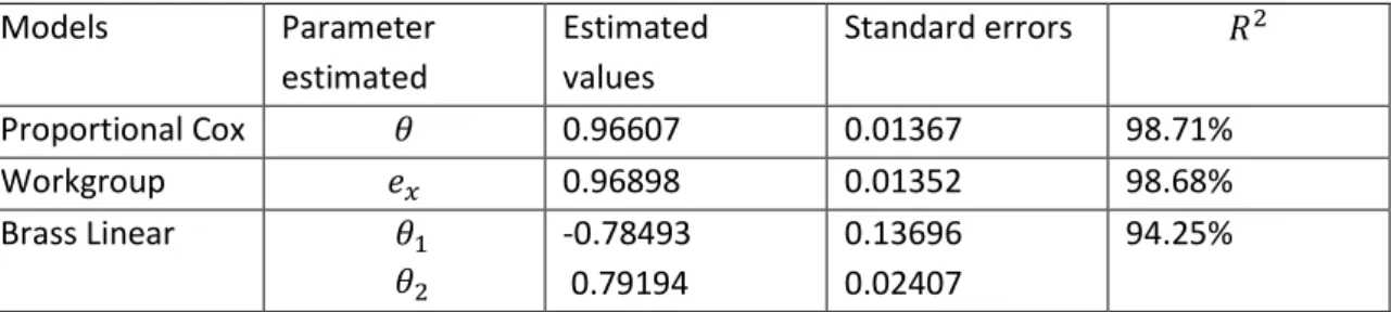
5 Results of relational model for WC market 36
6 forecasted one year death probabilities for the combined model using the Proportional Cox Model
37
7 Results of relational model for AXA portfolio 37
8 Forecasted one year death probabilities for the combined model using the Brass Linear model
38
9 Life expectancy for population and portfolio 38
8
CHAPTER 1: INTRODUCTION
1.1Worker’s Compensation: Compensations and Annuities
This report is based on a six months internship carried out at the Actuarial Department of AXA Portugal. The purpose of the internship was to develop a stochastic model for the future mortality of pensioners in AXA worker’s compensation portfolio and to study the impact on the reserves using this stochastic model instead of the static life table (TV 73/77) currently being used.
In Portugal, Workers Compensation (WC) is mandatory according to Law No.98/2009 of September 4th: all employers must insure the risk (all employees) in an insurance company; also, all self-employees must subscribe WC insurance.
This line of business includes obligations to compensate the victim and/or respective beneficiaries in case of accidents at work or if occupational diseases occur, from which a disability situation results (also including rehabilitation and reintegration). The accident on the
journey between the employee’s residence and the workplace and vice versa, and other
specific circumstances, for example, when the accident occurred between the workplace and the place where the employee takes meals, are also covered.
The nature of the resulting disability may be temporary or permanent. The temporary disability may be partial or absolute. The permanent disability may be partial, permanent for usual work or permanent for any work.
To make it easier for the readers to understand this issue, we will divide the losses in two parts: compensations and annuities.
Compensations:
The right to reparation includes the following forms: in kind and in cash. In kind, the main benefits are medical, pharmaceutical and hospital assistance needed to restore health and work capacity. Included are also transportation and accommodation, technical help for functional disabilities, thermal treatments and dependent relatives’ psychological assistance. All compensations provided by law, such as, compensation for temporary disability, death and funeral expenses, and subsidies for high disability (above 70%), house adaptation, rehabilitation and social integration are paid in cash.
9
Annuities:
Financial compensations for permanent disability are more complex because they include not only the victim but they may include other beneficiaries (orphans, husband/wife, parents or equivalents that live together and have earnings below the social pension). In Portugal this takes a significantly different character from what is found in most European countries (Belgium, Finland and Denmark are the exceptions that we know similar to Portugal). The management of this risk is maintained in Property and Casualty team (P&C) and it is present on P&C Balance sheet. The Law defines that in absolute permanent disability for any kind of work, the victim has the right to an annual pension equal to 80% of the salary and can add 10% per dependent person until the salary limit is reached.
In absolute permanent disability for usual work, the victim has the right to an annual pension between 50% and 70% of his/her salary, depending on the functional capacity to develop another compatible work. In partial permanent disability, the victim has the right to an annual pension equal to 70% of his salary devaluated by the degree of ability. Providing additional support for third person is assigned to victims without the capacity for basic daily needs. In case of death, the family or equivalent beneficiaries have the right to compensation:
–Husband/Wife or equivalent beneficiaries: compensation is 30% of the victim’s salary until
the retirement age of the beneficiary and 40% above retirement age or when disability or chronic illness is verified;
–Orphans: compensation is 20% of victim’s salary if there is only one; it’s 40% if there are two
orphans; and 50% if there are three or more orphans (may be 80% for orphans of both parents). The orphans have the right for compensation until 25 years old as long as they are students. Orphans are entitled to a pension for life in case of disability or chronic illness;
– Parents or equivalent beneficiaries: compensation is 10% of the victim’s salary for each beneficiary, limited to 30% of the salary. When there isn’t husband/wife or orphans, the parents or equivalents earn 15% for each until retirement age and 20% above retirement age or when disability or chronic illness is verified (however limited to 80%);
There are two types of pensions: the compulsorily recoverable and the not compulsorily recoverable. A pension is compulsorily recoverable for a victim when there is less than 30% of disability and the pension amount per year is less than six times the minimal national salary. For other beneficiaries (except orphans) only the second condition applies. On the other hand, a pension can be partially recoverable for victims if they have 30% or more of disability. The pensions for the other beneficiaries can be partially recoverable if the pension leftover is not less than six times the minimal national salary and capital redemption cannot be more than the capital that results of 30% of disability. The law defines that the mathematical provisions for compulsory recoverable and partial recoverable are calculated applying the following conditions: mortality table – TD 88/90 and rate of interest – 5.25% (maybe with rate of management).
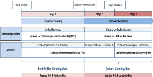
10 The figure below shows the framework for WC reserve.
FIGURE 1: WORKER’S COMPENSATION FRAMEWORK: RESERVES TYPES
Source: AXA documentations
1.2
Reserving for
worker’s
compensation
The Instituto de Seguros de Portugal (ISP) requires that Insurers have in their balance sheet mathematical reserves for permanent disability estimated from the date of occurrence of the accident. When estimated disability estimated is less 30% the annuity is paid as a lump sum (compulsory) and the capital to be paid after judge decision is calculated with legal parameters. Otherwise, insures must use best estimate parameters based on actuarial studies to evaluate it.
AXA Portugal presently uses the following parameters in this case:
Mortality table Interest rate Disability ≤30% Legal parameters TD 88/90 5.25% Disability ≥30% Best estimate
parameters
TD 73/77 4.5%
The actualization of the annuities due to inflation is assured by a public fund (Fundo de Acidentes de Trabalho - FAT).The Fund receives from companies two types of contributions:
0.15% of sum insured and 0.85% of capital redemption of pensions’ stock at December 31
(that includes the mathematical provision for third person’s assistance).The capital redemption
amount is calculated based on the following parameters: Mortality table – TD 88/90; Rate of interest – 5.25%; and Rate of management – 0%.The companies must predict the provision for
Future “FAT” in their Balance Sheet.
Insurers must also have in their balance sheet claims reserves for other compensations (medical expenses, daily compensations and other compensation).These reserves includes a
Work accident Disability consolidation Judge decision
Stage 1 Stage 2 Stage 3
Temporary disability Permanent disability
Pension "presumível" (estimated) Pension "definida" (estimated) Pension "Homologada" (definitive)
Other compesations
Annuities
Estimated Mathematical Reserve (PM) Definitive Mathematical Reserve (PM)
(mainly )Non Life obligations (mainly) Life obligations
Revision Risk & Longevity Risk Reserve Risk & Revision Risk
Medical Expenses Lifetime Medical Assistance
11
reserve for whole life medical assistance that is calculated using life techniques (best estimate parameters).
According to Brian et al. (2013), adverse reserve development in older accident years is a
persistent problem in the workers’ compensation industry. Predicting the final cost of workers'
compensation claims is particularly difficult due to the long period of time over which claimants receive statutory indemnity and medical benefit payments. Misestimating of reserves for these claims can result in financial reporting errors, claim settlement inequities, loss of reinsurance protection due to late reporting of large claims (through "sunset" clauses) as well as a drag on current earnings. The misestimating of reserves for lifetime workers' compensation cases can stem from many issues including:
• Insufficient historical loss development data. Some serious lifetime injury claims can stay
open for several decades, but only limited historical loss experience may be available for analysis (e.g., 10 to 20 years).
• Significant impact of inflation on future costs. Generally, claims adjusters establish case
reserves based on today's costs without consideration of future indemnity benefit escalation and medical inflation. Compounding this issue is the relatively high workers’ compensation medical escalation rate (though tempered somewhat in very recent years) compared to general or medical consumer price indices (CPIs).
• Increases in medical utilization over time. Case reserves often do not anticipate future
intermittent medical costs such as surgeries, prosthetic replacements, and the high cost of end-of-life care. Other significant costs, such as those resulting from technology improvements, new treatments and greater use of expensive prescription narcotics also can contribute to inadequate case reserves.
• Use of outdated or static life tables. Even if case reserves reflect mortality considerations for
lifetime claims, often the mortality assumptions do not reflect future improvements in life expectancy. Also, the averaging nature of a simplistic life expectancy approach generally underestimates gross claim costs in an inflationary environment (i.e., the impact on costs of claimants dying before and after the life expectancy is not offsetting) and changes the distribution of losses in various layers.
• Industry case reserving practices. Industry case reserving philosophies and practices vary
widely and can lead to different incurred development patterns by company. For example, some organizations may only case reserve for a fixed number of years of payments (e.g., 5
years) or to a “settlement” value instead of an “ultimate value,” leading to continual case reserve increases or “stair stepping.”
We shall concentrate our work on the source of misestimating stemming from Outdated or static life tables because that was the reason for the internship.
12
leading to the necessity of including an additional effort on the part of contribution (s) of member (s).To cater for this, managing bodies of pension funds should choose the mortality table that best suits the profile of the population concerned. It would therefore be expected to seek somehow use dynamic tables, and not static tables TV 73/77.
The goal of this report is twofold. First we will derive a model for the mortality in the pensions portfolio of AXA, which allows for a forecast of the future mortality in this portfolio. Basically this will be done by developing two separate models and then integrating them. We will start by assessing the longevity of the Portuguese population as a whole, based on data of this group. For forecasting future mortality in the Portuguese population I will use the Poisson Lee-Carter method. Subsequently the effects of adverse selection in the AXA pensions portfolio will be implemented. These effects will be estimated by comparing past mortality in the portfolio to past population mortality. Combining the longevity projections and the effects of adverse selection future mortality in the portfolio will be forecasted. The resulting mortality model is then specific for the pensions portfolio of AXA. Secondly, this model will be used to quantify the amount of capital AXA should hold to cover their longevity risk for reserving not compulsorily recoverable pensions. The results for this internal model are then compared to those from the static table (TV 73/77) approach. On the basis of this comparison, conclusions recommendations will be made.
13
CHAPTER 2: LITERATURE REVIEW
Previous research on worker’s compensation reserving has several discussions around the
need to consider the improvement of mortality over time, with recent papers providing deeper analyses of other key assumptions and more detailed instructions on how to build a mortality model. In 1971, Ferguson points out the necessity of considering mortality in long-term pension-type workers' compensation awards. The author notes that in the calculation of tabular reserves for long term pension type awards special care must be used when an excess of loss reinsurance coverage is involved. The various reserves are calculated by breaking the gross or direct reserves (total expected payment) into its component pieces (direct reserve = net reserve + ceded reserve).The net reserve must be based on a temporary life annuity, thus taking into account both the mortality and interest discounting. The ceded reserve is based on a deferred annuity; deferred by the number of years needed to exhaust the ceding company retention.
Steeneck (1996) provides an update to Ferguson’s paper, incorporating escalation of
indemnity benefits and medical inflation in mortality-based forecasts. Several illustrations provide some sensitivity analysis concerning the interaction of mortality and claim cost structure. Both indemnity and medical expenses are modeled by annuities. An argument is made for the inclusion of escalation of indemnity (where applicable) and medical inflation within the annuity mathematics to provide a proper forecast of the individual gross loss
and to layer that loss properly. This moves the “loss development” provision away from
IBNR (incurred but not reported) reserves and into case reserves, providing greater accuracy and clarity to experience. This applies to gross, retrocessional, and net claim reserves.
Snader (1987) expands on the use of life contingency concepts in establishing reserves for claimants requiring lifetime medical care using a three phase approach-claim evaluation, medical evaluation and actuarial evaluation. This paper provides a comprehensive discussion of mortality modeling, including considerations for selecting key assumptions such as inflation, life expectancy, discounting and medical.
Gillam (1993) focuses on mortality assumptions in his discussion of the NCCI Special Call for Injured Worker Mortality Data in 1987 and 1988 and the ensuing analysis of that data. He concluded that differences in mortality, while significant, did not, at that time, imply significant redundancy or inadequacy of the tabular reserves.
14
out, and that this deterministic parameter produces biased results. In low reinsurance layers, the commutation amount is overstated, and ín high layers it is understated. By removing deterministic assumptions from the calculation, bias is removed from the results.
In his discussion of "ultimate" loss reserves (i.e., case plus IBNR reserves estimated on an individual claim basis) in the context of runoff operations, Kahn (2002) comments on a number of important considerations, including medical escalation and longevity of claimants, that may impact model scenarios.
Sherman and Diss (2005) comment on medical cost severities, escalation rates, and
mortality rates used to estimate a workers’ compensation tail for the medical component
of permanent disability claims. In this paper, the authors demonstrate that case reserves estimated based on the expected year of death (life expectancy approach) are significantly less than the expected value of such reserves using a life contingency cash flow approach.
Brian et al. (2013), provide a practical framework to construct mortality- based approach
to model lifetime worker’s compensation claims including a detailed discussion of the key assumptions. According to them the mortality model included nine major steps amongst which were the applications of mortality assumptions to undiscounted cash flows. Just as Sherman and Diss (2005), they also noted that the life expectancy (instead of the life contingency) approach underestimates the future liability and thus the reserves.
“Just as it is wrong to assume medical usage and inflation are fixed, so it is wrong to assume that a claimant’s life-span is fixed. Assuming a deterministic life-span leads to inaccurate calculations. Likewise, assuming deterministic medical care and inflation will lead to inaccurate calculations. A deterministic life span implies that high layers of reinsurance will not be hit, when they do, in fact, have a chance of getting hit if the
claimant lives long enough.” (Brian et al., 2013, page 16).
The above literature on worker’s compensation reserving tend to center around three specific problems: selecting a mortality table to use for computation of the reserves taking into consideration the mortality improvement over time; the applicability of this mortality table to the portfolio (claimant) population; assessing the impact (of using static versus dynamic mortality tables) on the future liability and thus the reserves. The literature reviewed which discussed such problems is presented in the preceding paragraphs.
The literature on the study of dynamic mortality is quite wide with several authors having different contributions to the subject. In the past, mortality patterns were parameterized in the form of different laws. One of them is the Gompertz-Makeham law. This assumes that the logarithm of mortality approximates a straight line when viewed over age. This law, already developed in the 19th century, seems to hold well for ages between 30 and
100 (Peters et al., 2012).As mortality rates have rapidly declined in the 20th century, the
15
component needed to be expanded with a time component as well. Lee and Carter (1992)
have developed a very influential and widely used model in this respect. Using central
mortality rates in the United States of America, the authors presented an extrapolative model that describe the mortality of the population using a single index, designed with time-series forecasting methods. By the method of singular value decomposition, which enables the achievement of a solution of least squares, found that the result represented clearly the pattern of mortality in the study. In short, the Lee-Carter method assumes the existence of a time effect in log mortality rates, meaning that death rates in a population have a strong tendency to move up or down together over time. This indeed seems to apply to
low-mortality countries (Pitacco et al., 2009).The Lee-Carter method does not only allow for
the calculation of point estimates of future rates of mortality and life expectancies, but also for the determination of confidence intervals.
Later, Lee (2000) reviewed the model, showing applications to American, Chilean and Canadian population. Some extensions in the original model are described, in particular the breakdown by gender, as the template was initially applied to total population. The author mentions that there are several population breakdown possibilities, but the most simple and intuitive way is the separate treatment of men and women, applying the model independently to each genus. Lee (2000) thus showed that the original Lee-Carter method performed well in explaining the rise in life expectancy in the US in the period 1989-1997.
Many alterations have been proposed in the literature to either improve the statistical soundness of the model or to come to a better fit. Brouhns et al. (2002) for instance propose the Poisson model. This model is very similar to the Lee-Carter model, but models the number of deaths conditional on the exposure-to-risk as a Poisson random variable, whereas Lee and Carter model the central death rates as a random variable. They used maximum likelihood estimation to estimate the parameters, instead of resorting to the method of singular value decomposition originally applied in Lee-Carter (1992). Specifically, the original method is embedded in a Poisson regression model, which is perfectly suited for age–sex-specific mortality rates. This model is fitted for each sex to a set of age-specific Belgian death rates. A time-varying index of mortality is forecasted in an ARIMA framework. These forecasts are used to generate projected age-specific mortality rates, life expectancies and life annuities net single premiums. Finally, a Brass-type relational model (Brass 1974) is proposed to adapt the
projections to the annuitant’s population, allowing for estimating the cost of adverse selection
in the Belgian whole life annuity market.
16
compared to the Lee-Carter method is that it does not impose perfect correlation of changes in mortality at different ages from one year to the next (Pitacco et al., 2009).Plat (2009a) proposes a model which aims to combine the strong points of the Lee-Carter model and the CBD-model and which seems to provide a better fit than those models, however being slightly more complex.
Estimating the parameters has now become significantly more difficult than in the standard Lee-Carter setting, but it also makes the model more flexible. Besides including an extra time component, one could also include a cohort effect in a mortality model. Renshaw and Haberman (2006) do this for the Lee-Carter method, coming up with an Age Period Cohort (APC) model. Cairns et al. (2009) propose an alteration of the CBD-model to include a cohort effect. When there is a cohort effect present in mortality for a specific population, people born in a certain year or period experience significantly different changes in mortality than other people in the population. A cohort effect thus differs from a time effect, as the latter holds for the entire population. Haberman and Renshaw (2011) argue that including a cohort parameter can lead to more accurate projections, but only for countries for which there indeed exists a significant cohort effect. Typically the UK is considered as such a country. For the Portugal, there is as far as I know no conclusive evidence for the existence of a cohort effect (Coelho et al. 2010).
In the literature, a lot of research concerning mortality patterns of entire populations (as discussed above) is performed. These models can be used to predict future mortality rates and the uncertainty (particularly the longevity risk) surrounding these estimates. For insurers (and pension funds) however, it is almost equally important to know how mortality in their portfolio relates to general mortality in the country in which they are active. Therefore, also models have been developed to quantify these specific relations. It should however be noted that the number of papers written in this field is far less than the number of papers written on general mortality patterns. This would not be a problem if the data set of the insurer is of such a size that it can be seen as a specific population itself (not only in number of clients, but also in number of years for which data is available).In that case, the insurer can just apply one of the models discussed before to its own data set. Typically, however, the number of clients is considerably smaller and reliable data is only available for a small number of years. This is why an insurer will often need to revert to a model for population mortality to predict future development in mortality rates. The specific relation between mortality in the portfolio and mortality in the population can then be applied to this model (Wijk, 2012).
17
al. (2004) make a collection of various relational models, including a model of Cox proportional hazards and the relational model Brass (Brass, 1974) which applied to several data sets.
Pitacco et al. (2009) on the other hand suggest that differences in mortality between different socio-economic groups have widened over time. In the same paper, Pitacco et al. (2009) propose a new model for portfolio mortality which assumes the rate of decline in mortality to be the same for both the general and the insured population. Also, they assume the relation between population mortality and portfolio mortality to be constant over time. They consider mortality data in Belgium, distinguished by gender and by type of annuity (individual or group).They find coefficients of determination R2 between 97.2% and 99.8% for males and females respectively. Note that in all these papers the analysis is limited to the ages 65-98.Confidence intervals for the regression is constructed as for the Cox Proportional Hazard model.
Another important model is the one developed by Plat (2009).It makes no assumption about the relation between population and portfolio mortality being constant over time or not. Plat (2009) wants to estimate portfolio mortality factors for ages x = x1, ..., xm and years t = t1, ..., tn. For every year t, the author employs a regression model to approximate different vectors of portfolio mortality factors in year t. This regression model is fitted using Generalized (or Weighted) Least Squares based on the observed number of deaths. Plat (2009) applies this model to data from a large portfolio of about 100,000 insured males above the age of 65, and to a medium-sized portfolio of about 45,000 insured males aged above 65.For these portfolios he finds an AR(1) as the most appropriate to model the relationship between population and portfolio mortality.
Unlike in the previously mentioned relational models, Plat (2009) does find ways to combine the stochastic characteristics of both the population and portfolio mortality model. In order to simulate mortality rates for both the population and the portfolio, he needs to know more about the correlations. He uses the technique of Seemingly Unrelated Regression (SUR), which imposes the need to use the same historical observation periods for both population and portfolio mortality. The technique of SUR does not require the processes to be similar, hence the name. The combined processes can then be fitted by first estimating the parameters equation by equation, by means of Ordinary Least Squares. In this way, both the uncertainty in the population mortality model and the uncertainty in the portfolio mortality model are represented in the combined model.
18
disappeared at age 104.5.Between ages 94.5 and 104.5, PLT assumes a linear relation, which they extrapolate until value 1 is reached. For men, PLT finds the relation for ages 29.5-94.5 to be linear. For women however they find a quadratic fit. PLT is able to provide life expectancies in 2058 (the final year of their projection) for people with pension insurance at one of the companies that have provided data. They find a (period) life expectancy at birth of 87.93 years for men and of 88.90 years for women. Remaining life expectancies at age 65 in 2058 are 23.77 years for men and 25.39 years for women.
To close this chapter, the approach of assessing the impact on the future liability and thus the
reserves of worker’s compensation using dynamic mortality tables rather than static ones
(Brian et al.2013).The authors express the difference in life expectancy of using different mortality tables. They concluded that a mortality-based approach is a valuable alternative to traditional property/casualty methods for estimating the future liability for mature claims with
stable future annual payments, such as lifetime workers’ compensation claims. Actuaries can
19
CHAPTER 3: PROJECTIONS OF MORTALITY
3.1 Stochastic Mortality Rates
There is a vast literature on stochastic modeling of mortality rates. Often used models are for example those of Lee and Carter (1992), Brouhns et al (2002), Renshaw and Haberman (2006), Cairns et al (2006a), as already stated in the literature review. These models are generally tested on a long history of mortality rates for large country populations, such as the United Kingdom or the United States. However, the ultimate goal is to quantify the risks for specific insurance portfolios.
In practice, however there is often not enough insurance portfolio specific mortality data to fit such stochastic mortality models reliably, because:
The historical period for which observed mortality rates for the insurance portfolio are available is usually shorter, often in a range of only 5 to 15 years.
The number of people in an insurance portfolio is much less than the country population.
So fitting the before mentioned stochastic mortality models to the limited mortality data of insurers, measured in insured amounts, will in many cases not lead to reliable results. In practice, this issue is often solved by applying a (deterministic) portfolio experience factor to projected (stochastic) mortality rates of the whole country population. We will thus model population mortality and portfolio specific mortality separately by first modelling the population mortality stochastically and later applying a deterministic portfolio factor to these projected stochastic population rates.
The following paragraphs present explanation of some useful terms, the data used, models and results from the estimation of the mortality of the Portuguese population and that for the Portfolio of Workers Compensation in Portugal and AXA.
3.2 EXPLANATION OF TERMS
In this section we will briefly explain some terms commonly used in mortality studies and which will be used throughout this report as well.
Exposure-to-risk: the exposure-to-risk 𝐸𝑥,𝑡, denotes the number of person years lived
during year t by people aged x at the start of the year. Assuming that people who die during a year have on average been alive during half of the year, the exposure-to-risk can be approximated by the number of survivors plus half the number of deaths in this group.
Central death rate: the central death rate 𝑚𝑥,𝑡 is defined as the total number of
people aged x who have died during year t(𝐷𝑥,𝑡) divided by the exposure-to-risk of age group x during year t. In formula: 𝑚𝑥,𝑡= 𝐷𝑥,𝑡/ 𝐸𝑥,𝑡 .
Death probability: the probability 𝑞𝑥,𝑡 that an individual aged x at the start of year t
s-20
year death probability (probability of dying within s years) after having reached age x in year t by 𝑠𝑞𝑥,𝑡.From now on, the term death probability will refer to a one-year death probability.
Survival probability: the survival probability 𝑝𝑥,𝑡 (the probability that a person aged x
will survive year t), is defined by 𝑝𝑥,𝑡= 1 − 𝑞𝑥,𝑡.Like for the death probabilities, one can also define the probability of surviving an additional s years after having reached year t by 𝑠𝑝𝑥,𝑡= 1 − 𝑠𝑞𝑥,𝑡.In applications s will typically be an integer, but it need not be. Force of mortality: the force of mortality μ𝑥,𝑡is defined by μ𝑥,𝑡= lim𝑠 ↓0 𝑠𝑞𝑥,𝑡/𝑠.It is
also referred to as the instantaneous rate of mortality at the age x in the year t. A typical assumption in the literature (for example Wijk 2012) is that the force of mortality is piecewise constant. We will also adopt this assumption, which is an essential one when the analysis is done forage groups with widths of one year. This assumption implies that the force of mortality becomes equal to the central death rate
𝑚𝑥,𝑡.
Period life expectancy: the (remaining) life expectancy calculated for a person in year
t, based on mortality rates which hold for year t. For instance if this person is aged 40 in year t, the survival probability to reach the age 50 in year t + 10 will entirely be based on the survival probabilities for people aged 41, 42, etc.in year t. For a person aged x in year t, the remaining period life expectancy 𝑒𝑥,𝑡 is defined by:
𝑒𝑥,𝑡 =∑ω−x𝜏=1 𝜏𝑝𝑥,𝑡+ 1/2
whereω denotes the maximum age an individual can reach. The first term calculates the number of complete years lived, the half is to compensate for the fact that, on average, a person dies half a year after the last and half a year before his next birthday. Note that the maximum age to be obtained is of course unknown, so typically an assumption is made. Throughout this report ω equals 110.
Cohort life expectancy: as above, but then cohort mortality rates are used. This means
21
3.3 PROJECTION OF PORTUGUESE POPULATION MORTALITY
3.3.1 DATA
Mortality data that we have used for the population longevity model comes from Human Mortality Database (HMD), which makes use of numbers provided by University of California Berkeley (Institute for Demographic Research).We have used total data for men and women. The sample covers the period starting in 1940 (t = t1) and ending in 2012 (t = tn), which is the latest year for which data from HMD is available. Death rates are provided for one-year age intervals and one-year period intervals. The first age group (x = x1) is that of persons aged 0, the last age group (x = xm) is that of persons aged 110. HMD provides data up to age group 110+.
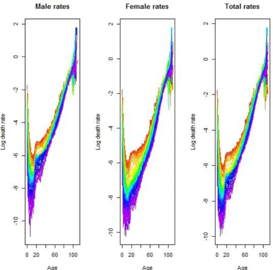
The following figures report for the Portuguese population the pattern of logarithm of death rates according to age and time. Several behaviors are shown respectively for male, female and total population.
22
For all countries and for males, females and the total population, the values of 𝑞𝑥 follow exactly the same pattern as a function of age, x. Figure 1 shows the Portuguese mortality rates for males, females and the total population. Note that we have plotted these on a logarithmic scale in order to highlight the main features. Also, although the information plotted consists of values of 𝑞𝑥 for x = 0, 1, ..., 110, we have plotted a continuous line as this gives a clearer representation. We note the following points from Figure 2 (see Dickson et al. 2011):
The value of 𝑞0 is relatively high. Mortality rates immediately following birth, perinatal mortality, are high due to complications arising from the later stages of pregnancy and from the birth process itself. The value of 𝑞𝑥 does not reach this level again until about age 80.
As expected the average mortality grows when age increases.
The rate of mortality is much lower after the first year, less than 10% of its level in the first year, and declines until around age 10.
Furthermore it is clearly visible the young mortality hump in the age-range (15,20) due to accidental deaths.
Mortality rates increase from age 10, with the accident hump creating a relatively large increase between ages 10 and 20, a more modest increase from ages 20 to 40, and then steady increases from age 4
Secondly, an initial exploration for trends in the data was conducted by plotting the logarithm of empirical mortality rates against calendar year for each age separately.
23
Figure 3 confirms there is a pronounced increase in the rate of improvement in mortality, stemming from the 1940s, in all age bands. This is a feature that was noted also by Wilmoth (2000) for the USA and Lee (2000).For both males and females and for the total population, there is a pronounced decrease in the rate at which mortality has been improving over the past quarter century, compared with the preceding quarter century.
3.3.2 MODELS
Given an appropriate model, forecasts of the single parameter could be then used to generate forecasts of the level and age distribution of mortality for the next few decades, Lee and Carter (1992).There are several candidates for the model.
We have decided to use three different models to predict future mortality of the general Portuguese population. The models are: the Original Lee-Carter method (Lee and Carter, 1992) with Gaussian errors, the Poisson Lee-Carter method (Brouhns et al., 2002) and the age-period-cohort (APC) variant of the Lee-Carter method including a cohort effect (Renshaw and Haberman 2006).Over the years the Lee-Carter method has evolved following proposals by other scientists. The reason that we have chosen for the Lee-Carter method and its improvements is there are relatively simple model, but not less accurate compared to other models, Wijk (2012).
Model 1: The Lee-Carter Model (Lee and Carter, 1992)
The original Lee–Carter method was used to aggregate (sexes combined) US data. Carter and Lee (1992) implemented their model for males and females separately, showing that the two series are best treated as declining independently. Wilmoth (1993) applied Lee–Carter methods to forecast Japanese mortality and also experimented with variants of this model. Lee and Nault (1993) applied Lee–Carter methods to model Canadian mortality and Brouhns and Denuit (2001) did the same for Belgian statistics, Coelho et al. (2010) and Pateiro (2013) applied it to the Portuguese population. It should be noted that the Lee–Carter method does not attempt to incorporate assumptions about advances in medical science or specific environmental changes; no information other than previous history is taken into account. This means that this approach is unable to forecast sudden improvements in mortality due to the discovery of new medical treatments or revolutionary cures. Similarly, future deteriorations caused by epidemics, the apparition of new diseases or the aggravation of pollution cannot enter the model, Brouhns et al. (2002).
Model 2: The Poisson Lee-Carter Model (Brouhns et al., 2002)
The Poisson-Lee-Carter model has some advantages over the classical version of the model that make it especially attractive. First, the model explicitly recognizes the integer nature of
24
The Lee–Carter methodology is a mere extrapolation of past trends. All purely extrapolative forecasts assume that the future will be in some sense like the past. Some authors (see, Gutterman and Vanderhoof (1999)) severely criticized this approach because it seems to ignore underlying mechanisms. As pointed out by Wilmoth (2000), such a critique is valid only in so far as such mechanisms are understood with sufficient precision to offer a legitimate alternative method of prediction. The understanding of the complex interactions of social and biological factors that determine mortality levels being still imprecise, the extrapolative approach to prediction is particularly compelling in the case of human mortality.
Model 3: The Poisson Lee-Carter Model with cohort effects (Renshaw and Haberman, 2006)
In a more recent development, the basic setting has been further extended to include an additional bilinear term, containing a second period effect (as in Renshaw and Haberman, 2003b) or a cohort effect (as in Renshaw and Haberman, 2006). In particular, the latter approach sheds new light on the early 20th century England and Wales mortality patterns. Thus, the basic Lee-Carter model can be transformed into a more general framework in order to analyse the relationship between age and time and their joint impact on the mortality rates.
3.3.3 FITTING THE MODELS
Model 1: The Lee-Carter Model (Lee and Carter, 1992)
The Lee-Carter method (Lee and Carter, 1992) combines a demographic model, describing the historical change in mortality, a method for fitting the model and a time series model for the time component which is used for forecasting. The classical two-factor Lee-Carter model is
ln(𝑚𝑥,𝑡) = 𝛼𝑥+ 𝛽𝑥𝑘𝑡+ 𝜀𝑥,𝑡 (1)
where 𝑚𝑥,𝑡 denotes the central mortality rate at age x in year t. When model (1) is fitted by ordinary least-squares (OLS), interpretation of the parameters is quite simple.
𝛼𝑥: the fitted values of 𝛼𝑥 exactly equals the average of ln(𝑚𝑥,𝑡) over time t so that exponential is the general shape of the mortality Schedule.
𝛽𝑥: represents the age-specific patterns of mortality change. It indicates the sensitivity of the logarithm of the force of mortality at age x to variations in the time index 𝑘𝑡.
𝑘𝑡: represents the time trend.The actual forces of mortality change according to an overall mortality index 𝑘𝑡 modulated by an age response 𝛽𝑥 .The shape of the 𝛽𝑥profile tells which rates decline rapidly and which decline slowly over time in response of a change in 𝑘𝑡 .
The error term 𝜀𝑥,𝑡, with mean 0 and variance 𝜎𝜀2, reflects particular age-specific historical influence not captured in the model.
The equation underpinning the Lee-Carter model is known to be over parameterized. To ensure model identification, Lee and Carter (1992) add the following constraints to the parameters:
25
to obtain unique parameter estimates. As a result of these constraints, the parameter 𝛼𝑥 is calculated simply by averaging the ln(𝑚𝑥,𝑡) over time.
A) OLS estimation
The main statistical tool of Lee and Carter (1992) is least-squares estimation via singular value decomposition of the matrix of ln(𝑚𝑥,𝑡) .The model (1) is fitted to a matrix of age-specific observed forces of mortality using singular value decomposition (SVD).Specifically, the
𝛼𝑥′𝑠, 𝛽𝑥′𝑠 𝑎𝑛𝑑 𝑘𝑡′𝑠 are such that they minimize
∑ ( 𝑥,𝑡 ln(𝑚𝑥,𝑡) − 𝛼𝑥− 𝛽𝑥𝑘𝑡)2 (2)
It is worth mentioning that model (1) is not a simple regression model, since there are no observed covariates in the right-hand side. The minimization of (2) consists in taking for 𝛼𝑥the row average of the ln(𝑚𝑥,𝑡) ’s, and to get the 𝛽𝑥′𝑠 𝑎𝑛𝑑 𝑘𝑡′𝑠 from the first term of an SVD of the matrix ln(𝑚𝑥,𝑡) − 𝛼𝑥.This yields a single time-varying index of mortality 𝑘𝑡 .
Before proceeding directly to modeling the parameter 𝑘𝑡 as a time series process, the 𝑘𝑡′𝑠 are adjusted (taking 𝛼𝑥 and 𝛽𝑥 estimates as given) to reproduce the observed number of deaths
∑ 𝐷𝑥 𝑥,𝑡 i.e. the 𝑘𝑡′𝑠 solve the equation
∑ 𝐷𝑥 𝑥,𝑡= 𝐸𝑥,𝑡exp (𝛼𝑥+ 𝛽𝑥𝑘𝑡) (4)
So, the 𝑘𝑡′𝑠 are reestimated so that the resulting death rates (with the previously estimated
𝛼𝑥′𝑠 and 𝛽𝑥′𝑠 ) applied to the actual risk exposure, produce the total number of deaths actually observed in the data for the year t in question.
There are several advantages to make this second-stage estimate of the parameters 𝑘𝑡 .In particular, it avoids sizable discrepancies between predicted and actual deaths (occurring because the first step is based on logarithms of death rates).Other advantages are discussed by Lee (2000).
B) Modelling the Index of Mortality
Having developed and fitted the demographic model, we are now ready to move to the problem of forecasting. An important aspect of Lee–Carter methodology is that the time factor
𝑘𝑡 is intrinsically viewed as a stochastic process. To forecast, Lee and Carter assume that 𝛼𝑥 and 𝛽𝑥remain constant over time and forecast future values of 𝑘𝑡 using a standard ARIMA univariate time series model.
The first step is to find an appropriate ARIMA time series model for the mortality index 𝑘𝑡 . Box–Jenkins methodology (identification–estimation–diagnosis) is used to generate the appropriate ARIMA time series model for the mortality indexes of the various models estimated (see Box and Jenkins, 1970).These forecasts in turn yield projected age-specific mortality rates and life expectancies.
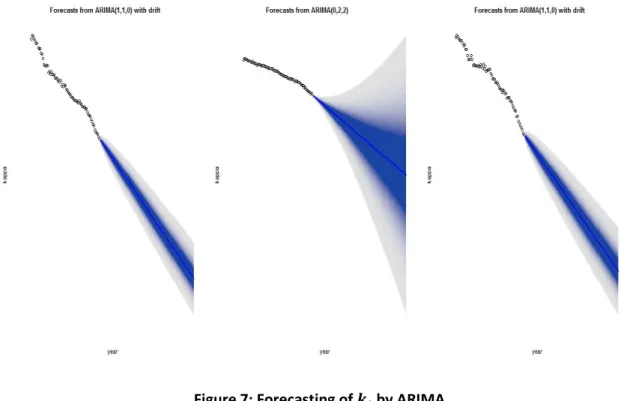
After carrying out the standard model identification procedures we can find that an ARIMA (1,1,0) with drift best describes the mortality index (see Appendix 3 for details).The ARIMA model is given by:
26
The constant term 𝒄𝒕 indicates the average annual change of 𝑘𝑡, and it is this change that drives the forecasts of the long-run change in mortality. The Ɛ𝒕 is the independent disturbance (random error).
Model 2: The Poisson Lee-Carter Model (Brouhns et al., 2002)
According to Alho (2000), the Lee-Carter model described in equation (1) above is not well suited to the situation of interest. As already mentioned, the main drawback of the OLS estimation via SVD is that the errors are assumed to be homoscedastic. This is related to the fact that for inference we are actually assuming that the errors are normally distributed, which is quite unrealistic. The logarithm of the observed force of mortality is much more variable at older ages than at younger ages because of the much smaller absolute number of deaths at older ages. Because the number of deaths is a counting random variable, according to Brillinger (1986), the Poisson assumption appears to be plausible, Brounhs et al. (2002).
The Poisson Lee-Carter Model assumes that the age-specific forces of mortality are constant within bands of age and time. More formally, given any integer age x and calendar year t, he assume that
𝜇𝑥+𝜖,𝑡+𝜏= 𝜇𝑥,𝑡 for 0≤Ɛ, 𝞽˂1
Under this constant force of mortality assumption, 𝜇𝑥,𝑡may be estimated as the quotient between the number of deaths and the number of exposed to the risk of dying or 𝐸𝑥,𝑡.Brouhns et al. (2002) developed a maximum likelihood estimation solution of the Lee-Carter model based on the assumption that 𝐷𝑥,𝑡, the number of deaths recorded at age x during calendar year t , follows a Poisson distribution, i.e.,
𝐷𝑥,𝑡~ Poisson(𝜇𝑥,𝑡𝐸𝑥,𝑡) (5) with
𝜇𝑥,𝑡 exp(𝛼𝑥𝛽𝑥𝑘𝑡
where the parameters are still subject to the constraints in equation (1). The meaning of
𝛼𝑥, 𝛽𝑥 and 𝑘𝑡 parameters is essentially the same as the classical Lee-Carter model.
A) Maximum likelihood estimation
The model preserves the log-bilinear structure for 𝑚𝑥,𝑡but replaces the classical assumptions on the error term 𝜀𝑥,𝑡 by a Poisson law for 𝐷𝑥,𝑡.In spite of this, parameters 𝛼𝑥, 𝛽𝑥and 𝑘𝑡 maintain,in essence, their original interpretation.Instead of resorting to SVD procedures, parameter estimates maximize the following log-likelihood function:
𝐿(𝛼𝑥, 𝛽𝑥, 𝑘𝑡)=∑𝑥𝑚𝑎𝑥𝑥 𝑚𝑖𝑛∑𝑡 𝑚𝑖𝑛𝑡𝑚𝑎𝑥{𝑑𝑥,𝑡(𝛼𝑥+𝛽𝑥𝑘𝑡) − 𝐸𝑥,𝑡exp (𝛼𝑥+𝛽𝑥𝑘𝑡)} + 𝑐 (7)
27
To forecast, as in the Lee–Carter method, we use the above time series methods to make long-run forecasts of age–sex-specific mortality rates.
B) Modelling the Index of Mortality
We do not modify the time series part of the Lee–Carter methodology. Estimates of 𝛼𝑥𝑎𝑛𝑑 𝛽𝑥, are used with forecasted 𝑘𝑡 to generate other lifetable functions.After carrying out the standard model identification procedures we can find that an ARIMA(0,2,2) without drift best describes the mortality index ( see Appendix 3 for details).The ARIMA model is given by:
𝒌𝒕− 𝒌𝒕−𝟏− 𝒌𝒕−𝟐= Ɛ𝒕+ 𝜽𝟏 Ɛ𝒕−𝟏+ 𝜽𝟐 Ɛ𝒕−𝟐
Model 3: The Poisson Lee-Carter Model with cohort effects (Renshaw and Haberman, 2006)
In the current application, we follow the APC modelling framework and fitting methodology proposed by Renshaw and Haberman (2006) that specifies the force of mortality by a generalized structure written as
𝜇𝑥,𝑡 = exp(𝛼𝑥+ 𝛽𝑥(0)(𝑖𝑡−𝑥) +𝛽𝑥(1)𝑘𝑡 ) (8)
where 𝛼𝑥 maps the main age profile of mortality and 𝑖𝑡−𝑥 and 𝑘𝑡represent the cohort and period effects, respectively; parameters 𝛽𝑥(0) and 𝛽𝑥(1) measure the corresponding interactions with age.
A) Maximum likelihood estimation
The parameter estimates maximize the following log-likelihood function:
𝐿(𝛼𝑥, 𝛽𝑥,𝑖𝑡−𝑥, 𝑘𝑡)=∑𝑥𝑚𝑎𝑥𝑥 𝑚𝑖𝑛∑𝑡 𝑚𝑖𝑛𝑡𝑚𝑎𝑥{𝑑𝑥,𝑡(𝛼𝑥+ 𝛽(0)𝑥 (𝑖𝑡−𝑥) + 𝛽𝑥(1)𝑘𝑡 ) − 𝐸𝑥,𝑡exp (𝛼𝑥+ 𝛽𝑥(0)(𝑖𝑡−𝑥) + 𝛽𝑥(1)𝑘𝑡 )} + 𝑐 (9) where c is a constant. To ensure model identification, we add the following constraints to the parameters:
∑𝑥 𝑚𝑎𝑥𝛽𝑥(0)
𝑥 𝑚𝑖𝑛 =∑𝑥 𝑚𝑎𝑥𝑥 𝑚𝑖𝑛 𝛽𝑥(1)=1, and ∑𝑥 𝑚𝑎𝑥𝑥 𝑚𝑖𝑛𝑘𝑡=0
As before, the presence of the log-bilinear term 𝛽𝑥(0)(𝑖𝑡−𝑥) and 𝛽𝑥(1)𝑘𝑡 in (8) prevents the estimation of model parameters using standard statistical packages that include Poisson regression. Because of this, we resort to an iterative algorithm for estimating log-bilinear models developed by Goodman (1979) based on a Newton-Raphson algorithm. Finally, a reparametrization of the model is necessary in order to guarantee that the parameter estimates for 𝛼𝑥, 𝛽𝑥(0), 𝛽𝑥(1),𝑘𝑡 generated by the ML procedure verify the model identification constraints.
28
Using the complete data set convergence could not be achieved and thus the deviance function could not be minimized. Thus in this application we make use of the data using a restricted age range from 18-85 so that convergence could be achieved, the deviance function minimized and the model parameters obtained.
B) Modelling the Index of Mortality
To forecast, as in the Lee–Carter method we use the same time series methods to make long-run forecasts of trend parameters 𝑖𝑡−𝑥 𝑎𝑛𝑑 𝑘𝑡.
After carrying out the standard model identification procedures we can find that an ARIMA(1,1,0) without drift best describes the mortality index (see Appendix 3 for details). The ARIMA model is given by:
𝒌𝒕− ∅𝟏𝒌𝒕−𝟏= 𝒄𝒕+ Ɛ𝒕+ Ɛ𝒕−𝟏.
3.3.4. RESULTS
In the previous section we have described the three Lee-Carter methods we have used in the estimation. In this section, the results of these approaches for modeling future mortality in the Portuguese population are presented and discussed.
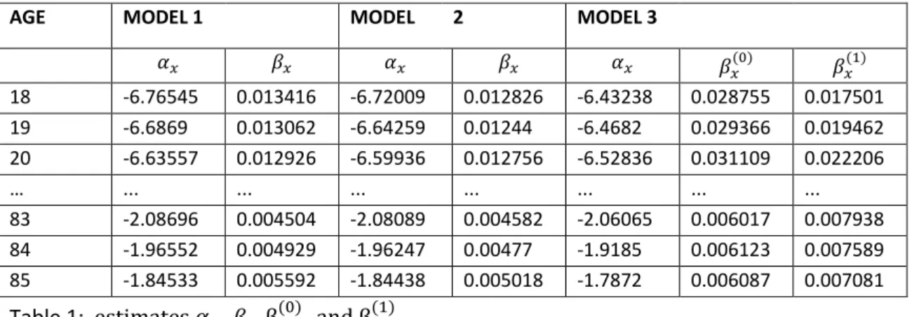
An extract of the estimated 𝛼𝑥 , 𝛽𝑥, βx(0) , and βx(1) (for the total population) of the different models is given in table 1 below. The full numerical values are presented in Appendix 2.
AGE MODEL 1 MODEL 2 MODEL 3
𝛼𝑥 𝛽𝑥 𝛼𝑥 𝛽𝑥 𝛼𝑥 𝛽𝑥(0) 𝛽𝑥(1)
18 -6.76545 0.013416 -6.72009 0.012826 -6.43238 0.028755 0.017501 19 -6.6869 0.013062 -6.64259 0.01244 -6.4682 0.029366 0.019462 20 -6.63557 0.012926 -6.59936 0.012756 -6.52836 0.031109 0.022206
… ... ... ... ... ... ... ...
83 -2.08696 0.004504 -2.08089 0.004582 -2.06065 0.006017 0.007938 84 -1.96552 0.004929 -1.96247 0.00477 -1.9185 0.006123 0.007589 85 -1.84533 0.005592 -1.84438 0.005018 -1.7872 0.006087 0.007081
Table 1: estimates 𝛼𝑥 , 𝛽𝑥, βx(0) , and βx(1)
An extract of the estimated 𝑖𝑡−𝑥 and 𝑘𝑡 (for the total population) of the different models is given in table 2 below. The full numerical values are presented in Appendix 2.
Year Model 1 Model 2 Model 3
𝑘𝑡 𝑘𝑡 𝑘𝑡 𝑖𝑡−𝑥
1940 74.578 65.958 0 53.577
1941 80.4121 73.121 3.2435 53.478
1942 78.69425 69.453 0.6468 53.380
… … … … …
2011 -76.894 -99.5736 -156.936 0
2012 -79.155 -98.1178 -158.53 0
29
The resulting values for the parameters of the ARIMA models are given in Table 2, for the κt ’s obtained via the classical Lee–Carter method, for the Poisson case and for the model with cohort effects. The detailed results are presented in Appendix 3.
Model 𝒄𝒕 ∅𝟏 𝜽𝟏 𝜽𝟐 Ɛ𝒕
Model 1 -2.1612 0.3116 0 0 0.1184
Model 2 0 0 -1.5482 0.6883 0.0929
Model 3 -1.7135 -0.3562 0 0 0.1118
Table 3: Estimates of parameters of ARIMA models
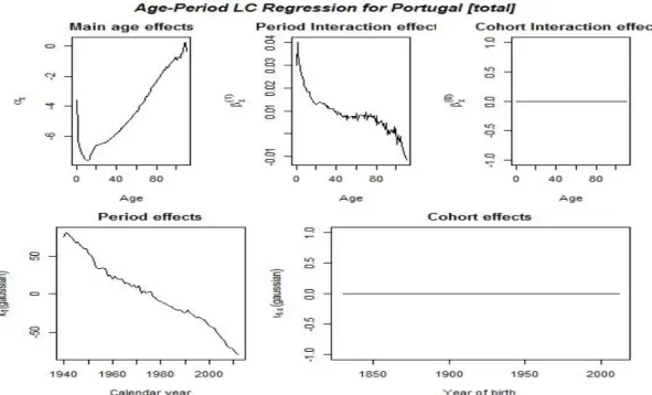
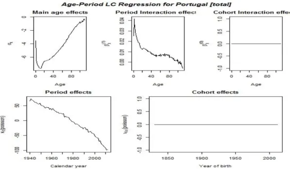
Figures 2, 3, 4 and 5 plot the estimated 𝛼𝑥, 𝛽𝑥(0), 𝛽𝑥(1),𝑘𝑡 and 𝑖𝑡−𝑥 (for the total population) of the diferente models.This clearly illustrates the fact that similar trends are observed. Appendix 2, contain the detailed numerical values.
30
Figure 5: Lee-Carter with Poisson Errors
31
Figure 7: Forecasting of 𝒌𝒕 by ARIMA
The figures indeed present a pattern for 𝛼𝑥 which is consistent with previous results in the literature, see for instance De Waegenaere et al. (2010). At age 0 mortality is quite high due to infant mortality, after which it is decreasing until the age of 10. Afterwards it is approximately
linearly increasing, except for the ‘accident hump’ noticeable for young adults. However when
cohort effects are taken into consideration the decrease is from 0 to 20 years thereafter there is a linear increase.
The pattern of βx(0) and 𝛽𝑥(1)shows that young children have profited most (high βx(0)) from the decrease in mortality over time. Again the pattern shows close resemblance with previous results in the literature, see for instance De Waegenaere et al. (2010a). Note also that variation in the value is higher for lower ages, showing that the mortality rates over time have varied more for the young.
Estimates for 𝑘𝑡 are initially obtained for years 1940-2012 and displayed in the figures. As expected, 𝑘𝑡 has a decreasing trend with the increment of time.
32
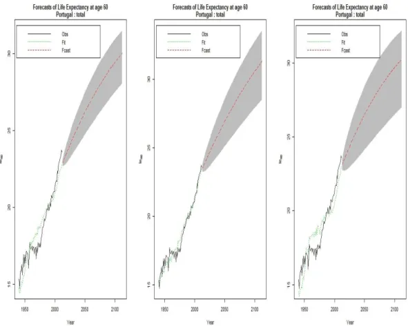
Figure 8: From left to right: observed, estimated and forecasted life expectancy of models 1,2 and 3.
Figure 8 shows that the Poisson Lee-Carter (model 2) has the best fit. We thus will use it as the base model to model the population mortality of the Portuguese market. The mortality rates obtained will then be used as reference rate to model the mortality rate of Workers compensation for the Portuguese market as well as the Portfolio of AXA in the next sections.
3.4 PROJECTION OF PORTFOLIO SPECIFIC MORTALITY FOR PORTUGUESE MARKET OF
PENSIONERS AND AXA PORTFOLIO OF PENSIONERS
33
development in mortality rates. The specific relation between mortality in the portfolio and mortality in the population can then be applied to this model ( Wijk,2012).In practice the issue of modelling portfolio mortality is solved by applying a deterministic portfolio experience factor to projected stochastic mortality rates of the whole population.
In this section we will discuss the way we model the mortality as experienced in the pension’s portfolio of both the Portuguese market and AXA Portugal .The first subsection is about the data we have used, the second is about the models we have adopted for our analysis, third estimation procedure and results and the last comments.
3.4.1 DATA
The data was provided by the Actuarial Department of AXA. The information for the Portuguese market as a whole spans the period from 2006 up to and including 2013 and that for AXA spans the period from 2006 up to and including 2014.Unfortunately the data from 2013 and 2014 is not of much use, since we have no access to population mortality data for these years and we can therefore not compare the mortality in population and portfolio for those years. This is why our analysis is only based on the years 2006 up to and including 2012. For every year 2006-2012, we were provided with the number of insureds per age("N.º pessoas expostas ao risco (EX)") and gender. Also, for every year we received the number of deaths per age (Mortalidade real) and gender. Using these numbers we could find the observed death probabilities for each age (central mortality rates and initial mortality rates).For example for AXA portfolio the initial and central mortality rate respectively are given
by 𝑞. 𝐴𝑋𝐴 =𝐷𝑒𝑎𝑡ℎ.𝐴𝑋𝐴
𝐸𝑥𝑝.𝐴𝑋𝐴 and 𝑚. 𝐴𝑋𝐴 = − log(1 − 𝑞. 𝐴𝑋𝐴).
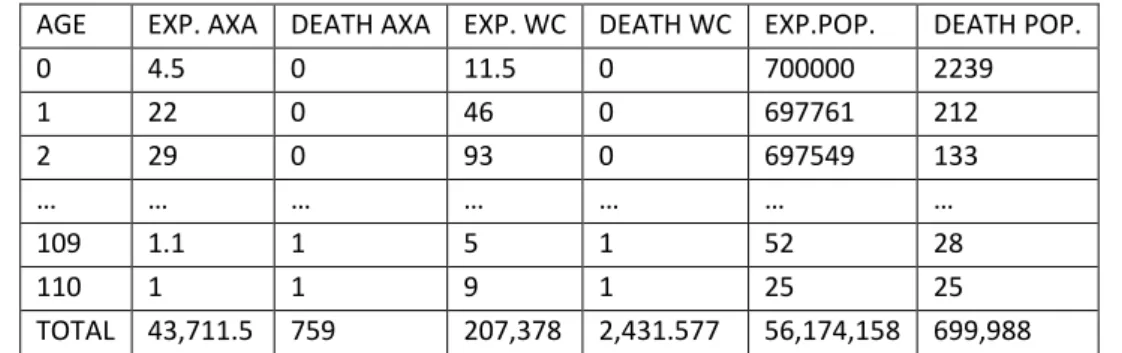
As the sample is not that big (number of deaths for AXA portfolio aggregated over all age groups and the total period: 759; number of deaths for pension portfolio of Portugal aggregated over all age groups and the total period: 2431) as compared to 699,988 for the whole Portuguese population, it was thus not possible to study the specific portfolio mortality for each year separately, hence we studied for the total time period. This same approach is applied by Wijk(2012), Brouhns et al. (2002) and Denuit(2007) in modelling portfolio mortality. An extract of the data is given below. The complete data set is given on Appendix 4.
AGE EXP. AXA DEATH AXA EXP. WC DEATH WC EXP.POP. DEATH POP.
0 4.5 0 11.5 0 700000 2239
1 22 0 46 0 697761 212
2 29 0 93 0 697549 133
… … … …
109 1.1 1 5 1 52 28
110 1 1 9 1 25 25
TOTAL 43,711.5 759 207,378 2,431.577 56,174,158 699,988