Dissertação S TRUCTURAL CHANGES IN DURATION OF BULL AND BEAR MARKETS

(1)

M

ESTRADO

ECONOMETRIA

APLICADA

E

PREVISÃO

T

RABALHO

F

INAL DE

M

ESTRADO

Dissertação

S

TRUCTURAL CHANGES IN DURATION OF BULL AND BEAR MARKETS

AND THEIR CONNECTION WITH BUSINESS CYCLES

J

OÃO

A

NTÓNIO

M

ENDES DA

C

RUZ

(2)

M

ESTRADO

ECONOMETRIA

APLICADA

E

PREVISÃO

T

RABALHO

F

INAL DE

M

ESTRADO

Dissertação

S

TRUCTURAL CHANGES IN DURATION OF BULL AND BEAR MARKETS

AND THEIR CONNECTION WITH BUSINESS CYCLES

J

OÃO

A

NTÓNIO

M

ENDES DA

C

RUZ

O

RIENTAÇÃO

:

P

ROFESSOR

D

OUTOR

J

OÃO

C

ARLOS

H

ENRIQUES DA

C

OSTA

N

ICOLAU

(3)

i

Structural Changes in Duration of Bull and Bear Markets and their Connection with Business Cycles

João Cruz

M.Sc.: Applied Econometrics and Forecasting Supervisor: João Nicolau

Abstract

The present work analyses relations between finance and

macroeconomics, aiming to answer how structural changes in duration of bull

and bear markets are connected with business cycles. In order to do so, we

review the structural change test proposed by Nicolau (2016) and introduce

two similar alternatives, which through a Monte Carlo simulation study, show

less over-rejection for some data generating processes, proving to be useful

in obtaining robust results.

We apply the tests to a database consisting on adjusted market

capitalization stock market indexes of 38 developed and emerging markets,

constructed by Morgan Stanley Capital International. In our results we find

several structural changes that seem to be linked to macroeconomic events,

furthermore, there is statistical evidence that decreases in duration of bull

market cycles anticipate the peak of business cycles.

Keywords: Bull and Bear Markets, Business Cycles, Duration of Bull and

Bear Market Cycles, Economic Crisis, MSCI, Structural Change Test.

(4)

ii

Structural Changes in Duration of Bull and Bear Markets and their Connection with Business Cycles

João Cruz

Mestrado: Econometria Aplicada e Previsão Orientação: João Nicolau

Resumo

O presente trabalho analisa relações entre finanças e macroeconomia,

procurando responder a como quebras de estrutura na duração dos

mercados bull e bear estão ligadas aos ciclos económicos. Para tal, é revisto

o teste de quebras de estrutura proposto por Nicolau (2016) e são

introduzidos dois testes alternativos, que através de um estudo de simulação

Monte Carlo, evidenciam menos sobre-rejeição para alguns processos

geradores de dados, provando ser úteis na obtenção de resultados robustos.

Aplicamos os testes a uma base de dados composta por índices

bolsistas de 38 mercados desenvolvidos e em emersão, ajustados à

capitalização de mercado, construídos pela Morgan Stanley Capital

International. Nos resultados obtidos encontramos várias quebras de

estrutura que revelam estar ligadas a eventos macroeconómicos, além disso,

existe evidência estatística de que decréscimos na duração dos ciclos de

mercado bull antecedem o pico dos ciclos económicos.

Palavras-Chave: Ciclos Económicos, Crises Económicas, Duração de Ciclos

de Mercados Bull e Bear, Mercados Bull e Bear, MSCI, Teste de Quebra de

Estrutura.

(5)

iii

Acknowledgements

Os meus agradecimentos vão para todos os que direta ou indiretamente

contribuíram para a elaboração deste trabalho, bem como para o meu

percurso académico e pessoal.

Em primeiro lugar agradeço aos professores do Mestrado em

Econometria Aplicada e Previsão, em especial ao meu orientador Professor

Doutor João Nicolau, por ter acompanhado a realização deste trabalho e por

ter prestado um valioso auxílioem qualquer questão decorrente do mesmo.

Agradeço também aos meus amigos e colegas, bem como aos meus

chefes no estágio que realizei na Autoridade Nacional de Comunicações

(ANACOM).

Por fim, um especial agradecimento à minha família e à Sofia pelo apoio

(6)

iv

List of Figures

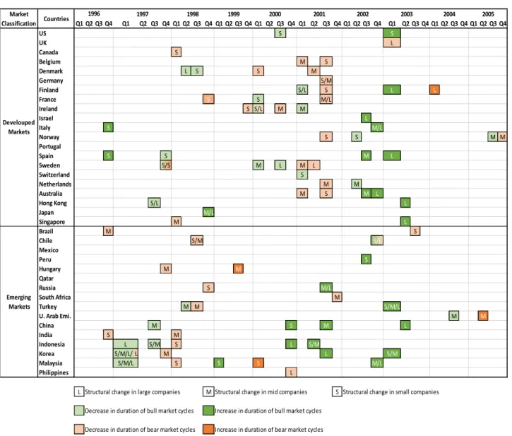
Figure 1 _– Structural changes in duration of bull and bear markets associated

with large, mid and small companies (1996 – 2005) ... 38

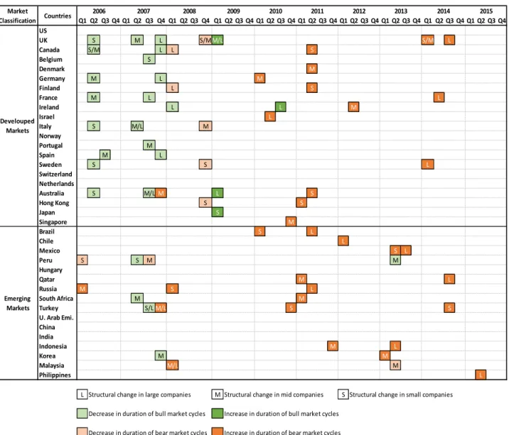
Figure 2 – Structural changes in duration of bull and bear markets associated

with large, mid and small companies (2006 – 2015) ... 39

List of Tables

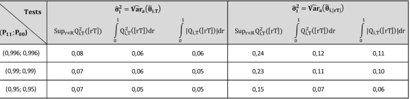
Table 1 – Real dimension associated with the structural change tests in

function of transition probabilities and choice of _σ̂_i2 (_{T = 3}₀₀₀₎ ... 40

function of transition probabilities and choice of _σ̂_i2₍_{T = 6}₀₀₀₎_{... 40}

function of transition probabilities and choice of σ̂_i2₍_{T = 15}₀₀₀₎_{... 40}

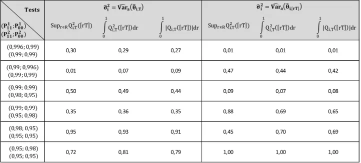
Table 4 – Power associated with the structural change tests in function of

transition probabilities and choice of _σ̂_i2₍_{T = 3}₀₀₀_{and breakpoint at the}_50th

percentile of the sample) ... 41

transition probabilities and choice of σ̂_i2₍_{T = 3}₀₀₀_{and breakpoint at the}_80th

transition probabilities and choice of _σ̂_i2₍_{T = 6}₀₀₀_{and breakpoint at the}_50th

(8)

vi

Table 7– Power associated with the structural change tests in function of

transition probabilities and choice of σ̂_i2₍_{T = 6}₀₀₀_{breakpoint at the}_80th

transition probabilities and choice of _σ̂_i2₍_{T = 15}₀₀₀_{and breakpoint at the}

50th percentile of the sample) ... 43

Table 9 _– Power associated with the structural change tests in function of

transition probabilities and choice of σ̂_i2₍_{T = 15}₀₀₀_{breakpoint at the}_80th

Table 10 – Data availability for developed markets ... 44

Table 11 – Data availability for emerging markets ... 45

Table 12 – Business cycles of markets with statistical evidence of DDBC .... 46

Table 13 _– Application of the Binomial test for evidence of dependence

(9)

1

1 _–

Introduction

One can characterize the financial market_s’ behaviour as bull and bear

(henceforth BB) markets: When studying a financial time series, it is possible

to recognize prolonged periods of time where an underlying trend seems to

be involved, these periods are related with the BB markets.

Although this feature has been quite studied by academics, there is not a

clear definition for it, nevertheless, the descriptions provided by Chauvet &

Potter (2000) and Sperandeo (1990) are useful for their simplicity and insight.

The former describe bullish (bearish) markets as periods of generally

increasing (decreasing) market prices, while the latter uses a similar

description, yet more precise, by defining a bull market as “a long-term (...)

upward price movement characterized by a series of higher intermediate (...)

highs interrupted by a series of higher intermediate lows”, and a bear market

as a _“long-term downtrend characterized by lower intermediate lows

interrupted by lower intermediate highs”.

One of the main reasons for the popularity of BB markets in the last

years is its importance in analysing and predicting financial markets, in this

sense, a great amount of work has been developed in identifying, modelling

and predicting BB markets. Lunde & Timmermann (2004), Maheu et al.

(2012), and Kole & Van Dijk (2017) are just some examples of the research

made in this area.

Less work has been achieved in analysing the BB markets duration, and

(10)

2

directly linked with the applications of BB markets as key components of

stock markets: If a structural change in the cycle duration is wrongly left

unconsidered, then an analysis based on BB markets will most likely be

compromised. For testing these structural changes only the test proposed by

Nicolau (2016) is known to date. Throughout the current work, this statistical

test is introduced, along with two simple alternatives derived from the former,

with a Monte Carlo simulation study being additionally carried out in order to

analyze the statistical properties of these tests.

This work’s empirical application intends to be a valid contribution in the

study of links between finance and macroeconomics, a field of research that

became especially active after the crisis of 2008 that affected economies

worldwide. To achieve so, the present work focuses in the analysis of the

connections between structural changes in the duration of BB markets and

the business cycles.

The upper mentioned statistical tests are applied to a database

consisting on adjusted market capitalization stock market indexes of 38

developed and emerging markets, and the breakpoints found are then

compared with the peaks and troughs verified in the business cycles as well

as periods of other global macroeconomic events. In this comparison, the

structural changes are then explained and justified considering both financial

and macroeconomic frameworks.

The remainder of this work is organized as follows: Section 2 introduces

some preliminary concepts on BB markets, specifically stationary first order

(11)

3

state. Section 3 presents several methods for the identification of BB markets.

Section 4 revises the existent structural change test in duration of BB markets

and presents two alternative tests. Additionally a simulation study is carried

out in this section, in order to ascertain the empirical size and power of these

tests, along with the critical values of the alternatives. Section 5 introduces

the empirical study where the tests are applied to adjusted market

capitalization stock market indexes and the connections between structural

changes in duration of BB markets and the business cycles are analyzed.

Section 6 presents extensions and possible further research to this work.

Section 7 revises the obtained results and concludes.

2 –

Preliminary Concepts on BB Markets

BB markets conveniently suit the probabilistic model proposed by Andrey

Markov. Let _{S_t_} be an indicator variable, which verifies _S_t _{= 1} if the stock

market is in a bull state and St = 0 if the stock market is in a bear state at

period _t. The evolution of _S_t is assumed throughout this work to be governed

by a stationary and ergodic first order Markov Chain Process. The transition

probabilities capture the temporal dependence of BB markets and are

presented as:

P(St = j|It−1) = P(St= j|St−1 = i) = pij ∀i, j = 0, 1 (2.1)

Where _I_t−1 is the σ-algebra generated by the available information at _{t −}

(12)

4

Since the transition probabilities are constant over time given {St}

stationary, the following one step probability transition matrix completely

describes the Markov Chain Process:

𝐒 ≔ [P_P(S(St = 1|St−1= 1) P(St = 0|St−1= 1)

t = 1|St−1= 0) P(St = 0|St−1= 0)] (2.2)

In order to introduce the concept of BB market durations, it is pertinent to

consider the following random variables:

TBull ≔ min(t > 0: St = 0|S0 = 1) ; TBear≔ min(t > 0: St = 1|S0 = 0) (2.3)

The variable _T_Bull represent the time of first passage to the bear state

given that the market started at a bull state, _T_Bear has an analogous

interpretation. Since the Markov chain is assumed to be stationary, the

expected value of the variables mentioned above is constant and given by:

θ1 ≔ E(TBull) =_{1 − p}1

11; θ0 ≔ E(TBear) =

1

1 − p00 (2.4)

See, for example, Taylor & Karlin (1998). Equation (2.4) shows the

expected time of permanency in the BB states related to a certain series, that

is, the duration of the BB market cycles. Intuitively, to test the hypothesis of

whether the BB market durations are constant over time or not, is to test if the

equality _θ_i,t _{= θ}_i holds for all _t. Such is a major focus of this current work, as

(13)

5

3 _–

Identification of BB Markets in a Time Series

Before introducing the structural change tests in duration of BB markets

and their applications, it is first necessary to present methods for the

identification of bullish and bearish states. To do so, there are two

distinguishable main approaches, one nonparametric and other based on a

parametric statistical model. The latter uses regime-switching models (see,

for example, Maheu et al. (2012)) which have their own advantages since

they give more depth into the process under study and allow a direct

statistical inference. However, these models and their results are dependent

on a correct specification, which is something not desirable in the present

work. It is preferred the use of a transparent and robust method of

identification, that solely reflects the tendency of the market. Such leads to

the use of nonparametric rules-based methods.

The two main algorithms in the literature are presented by Pagan &

Sossounov (2003) and Lunde & Timmerman (2004). The former’s approach is

based on the algorithm developed by Bry & Boschan (1971) for dating

business cycles and consists in the identification of peaks and troughs as well

as the adoption of duration censoring rules that restrict the minimal lengths of

any phase. Seeing that the method proposed by Lunde & Timmerman (2004)

does not impose such restrictions in the cycle’s durations, it will be selected

throughout this work for the identification of BB markets since it is preferred

(14)

6

To identify bullish (_S_t_{= 1}) and bearish (_S_t _{= 0}) states, the chosen

method uses two parameters, _λ₁ and _λ₂, as a way of measuring the

dimension of a rise (drop) in the time series to be considered a peak (trough).

Let the stock market be in a bullish state at _{t = t}₀, with _P_tMax₀ _{equal to its}

value at that period (_P_t₀) and consider the stopping time variables _τ_Max and

τMin defined by:

τMax = inf{t0+ τ: Pt0+τ≥ PtMax0 }

τMin = inf{t0+ τ: Pt0+τ < (1 − λ2)PtMax0 }

(3.1)

If _τ_Max _{< τ}_Min_,then set _P_tMax₀_+τ_Max _{= P}

t0+τMax and St = 1,∀ t ∈ {t0 +

1, … , t0+ τMax }, otherwise set PtMin0+τMin = Pt0+τMin and St = 0,∀ t ∈ {t0+

1, … , t0+ τMin }.

Similarly, with the stock market in a bearish state at _{t = t}₀, the stopping

time variables _τ_Max and _τ_Min are defined by:

τMin = inf{t0+ τ: Pt0+τ ≤ PtMin0 }

τMax = inf{t0+ τ: Pt0+τ > (1 + λ1)PtMin0

(3.2)

If _τ_Min_{< τ}_Max_,then set _P_tMin₀_+τ_Min _{= P}

t0+τMin and St= 0,∀ t ∈ {t0+

1, … , t0+ τMin}, otherwise set PtMax0+τMax = Pt0+τMax and St = 1,∀ t ∈ {t0+

1, … , t0+ τMax }.

By repeating the above set of rules the BB states are identified. Notice

that the algorithm simply defines bullish cycles as the movements of a time

series between two local maximums without significant drops in the middle, or

(15)

7

no duration restrictions are implied. The bearish cycles are analogously

defined.

The identification of BB markets through this algorithm depends on the

choice of (_λ₁; _λ₂). If this parameters are set too low, then small downward

(upward) movements during a bull (bear) cycle are considered a sign of a

transition to a bear (bull) state. Moreover, it is intended that the upward drift in

stock prices is considered, this is achievable by setting _λ₁ _{> λ}₂. Knowing this

concerns, throughout this work the values (_0,20; _0,15) are chosen for these

parameters.

4 –

Structural Change Tests in Duration of BB Markets

4.1 –

A Revision on Structural Change Tests in Duration of BB

Markets

In this section, the structural change test introduced by Nicolau (2016) is

presented.

This test aims to detect differences in the duration of BB markets

between two subsamples, that is, if the transition probabilities inherent to the

BB states have changed from one period to another.

When applied to the stock market, evidence of a structural change in a

specific date may prove that some sort of phenomenon led to an increase or

(16)

8

applications in understanding the relations linking some economical or

financial events and the stock market in study.

The test compares the estimated duration of the bull (bear) market cycle

using all _T observations, with the estimated durations using the first _{t ∈]w, T[}

observations, where _w is a start-up value to be explained during this section

and _T the sample size. This way, a great deviation between durations

represents an evidence of a structural change in the stability of the bull (bear)

cycle.

To estimate the duration of these cycles, consider the already presented

equation (2.4), with the transition probabilities _p_ii_{∀i = 0, 1} replaced by their

maximum likelihood estimates _p̂_ii:

θ̂1 =_{1 − p̂}1

11; θ̂0 =

1

1 − p̂00 (4.1.1)

Therefore, given the functional invariance propriety, _θ̂_i is the maximum

likelihood estimate of _θ_i, _{i ∈ {0, 1}.}

To obtain p̂ii, first consider the following initial probabilities:

p_u(0): = P(S0 = u), u ∈ {0,1} (4.1.2)

With _𝐒_𝐓+𝟏 _{= {S}₀_{, S}₁_{, … , S}_T_} a realization of length _{T + 1} of the stochastic

process _{S_t_}, the likelihood function based on _𝐒_𝐓+𝟏 is specified by:

L = pu(0)∏ pSk−1Sk

T

k=1

= pu(0)∏ pijnij 1

i,j=0

(17)

9

Where nij is the number of times that a transition from i to j is verified in

the sample. The log-likelihood function is given by:

log(L) = log(pu(0)) + ∑ nij 1

i,j=0

log(pij) (4.1.4)

The maximum likelihood estimator of the transition probability _p₁₁ is

obtained through:

𝜕 log 𝐿_𝜕p

11 = 0 ⇔

n11

p̂11−

n10

1 − p̂11= 0 ⇔

n11− n1p̂11

p̂11(1 − p̂11) = 0 ⇔ p̂11 =

n11

n1 (4.1.5)

Notice that n1 = n11+ n10, which is the number of 1’s found in the

realization _𝐒_𝐓+𝟏. In general, the estimates of _p̂_ij can analogously be obtained

by _p̂_ij ₌nij

ni, i, j ∈ {0, 1}. Consequently, equation (4.1.1) can be written as:

θ̂1 =_n n1

1− n11; θ̂0 =

n0

n0− n00 (4.1.6)

Under the stationary hypothesis specified in Section 2, and given that _θ̂_i

is the maximum likelihood estimator of θi, its asymptotic behavior for i ∈ {0, 1}

is:

θ̂i

….p….

→ θi (4.1.7)

√T(θ̂i− θi)

….d….

→ N (0,_{(1 − p}pii

ii)3πi) (4.1.8)

Where _{0 < p}_ii _{< 1} and _π_i_{: = P(S}_t_{= i)}. To prove equation (4.1.8) notice

that _√T(p̂_ii_{− p}_ii)….→ N (0,d…. pii(1−pii)

(18)

10

As mentioned before, the goal is to test whether the durations of the BB

markets are constant over time or if its structure has changed. To do so, let

θ1,t and θ0,t be the durations of a bull cycle and bear cycle at t, respectively,

and focus on observations _{t = ⌊rT⌋}, for _{r ∈ R}, a pre-specified compact subset

of _{(0, 1)}, where _[x] is the integer part of _x.

To test _H₀: _θ_i,⌊rT⌋ _{= θ}_i _{∀r ∈ R} (i.e. parameter constancy) against its

alternative _H₁: _θ_i,⌊rT⌋ _{≠ θ}_i for some _{r ∈ R}, the following statistic is crucial:

Qi,T(⌊rT⌋) = √⌊rT⌋ − w_{T − w ∗}⌊rT⌋_σ̂ i

2 ∗ (θ̂i,⌊rT⌋− θ̂i,T) (4.1.9)

For _{i ∈ {0, 1}}, with _σ̂_i2_{the maximum likelihood estimate of}_Var

a(θ̂i,T) =

pii

(1−pii)3πi. For the computation of Qi,T(⌊rT⌋) it will also be considered the case

where _σ̂_i2_{is the maximum likelihood estimate of}_Var

a(θ̂i,⌊rT⌋) (the asymptotic

variance of the estimated duration using the first ⌊rT⌋ elements in the sample),

with its results compared to the previous situation1_{. For the distribution of}

Qi,T(⌊rT⌋) let:

Zi,t= (1 − θi)St+ θiStSt−1

√Vara(θ̂i,T)πi(1 − pii)

(4.1.10)

Then, under the stationary assumption mentioned at the beginning of

Section 2, one can prove (see Nicolau (2016)):

1_{Differences should occur only for finite samples, given that asymptotically the use of}_Var_̂

a(θ̂i,T) and

(19)

11

Xi,T(1) = 1

√T∑ Zi,t

T

t=1

….d….

→ W(1) (4.1.11)

Xi,T(r) = 1

√T∑ Zi,t

⌊rT⌋

t=1

….d….

→ W(r) (4.1.12)

Finally, the distribution of _Q_i,T_(⌊rT⌋) is given by:

Qi,T(⌊rT⌋) Xi,T(r) − rXi,T(1)

….d….

→ W(r) − rW(1) (4.1.13)

The test statistic and respective asymptotic distribution are obtained

through the application of the continuous mapping theorem to equation

(4.1.13). This theorem states that for a function g: ℝm_{→ ℝ}p _{continuous in its}

domain and independent of T, the following applies:

XT

….d….

→ X ⇒ g(XT)

….d….

→ g(X) (4.1.14)

Therefore, equation (4.1.13) can be transformed as:

Supr∈RQ2_i,T(⌊rT⌋)….→ Supd…. r∈R[W(r) − rW(1)]2 (4.1.15)

Which holds under _H₀. To test for possible structural changes in the BB

markets stability, consider the result in equation (4.1.15).

The implementation of this test is straightforward: First, one needs the

series of 1’s and 0’s relative to the BB states inherent to the series in study

(consider the Lunde & Timmerman (2004) rules-based method, already

discussed in Section 3). The statistics Q2

i,T([rT]) for r ∈ R are obtained from

(20)

12

leads to the question of what value for _w should be chosen. While a small

value is associated with the impossibility of obtaining the statistics _Q2

i,T([rT])

for some _{r ∈ R}, for a large value of _w the breakpoint may be missed. The

choice of _w suggested is one that allows for the sample _{{1, … w}} to have at

least two state transitions as a way of avoiding the impossibility to calculate

the statistics _Q2

i,T(w), and the subsequent to it. With w chosen, obtain

{θ̂i,w, θ̂i,w+1, … , θ̂i,T} using the subsamples {1, … , w}, {1, … , w + 1},… , {1, … , T},

respectively. _σ̂_i2_{can be estimated either one time, using the whole sample,}

yielding _σ̂_i2 _{= Var}_̂

a(θ̂i,T) or multiple times using the above subsamples,

yielding σ̂_i2 _{= Var}_̂

a(θ̂i,⌊rT⌋). Finally, after the computation of {Q2_i,T(w), Q2_i,T(w +

1), … , Q2

i,T(T)}, the maximum value of this sequence is compared to the

corresponding critical value and in case _H₀: _θ_i,⌊rT⌋ _{= θ}_i _{∀r ∈ R} is rejected, the

estimate for the breakpoint is given by the period in which _Q2

i,T(⌊rT⌋) achieves

its maximum.

The critical values obtained through simulation are 1,46, 1,78 and 2,54,

for test sizes of 10%, 5% and 1%, respectively.

The tests to be introduced in the next section are based on equation

(4.1.13) and are also obtained through the continuous mapping theorem,

being very similar to the one previously presented. These tests essentially

differ from each other in the application of the theorem, which yields different

(21)

13

4.2 _–

Alternative Structural Change Tests in Duration of BB

Markets

The test presented previously uses the supremum squared value of

Qi,T(⌊rT⌋) as its test statistic, analogously, other test statistics can be obtained

from _Q_i,T_(⌊rT⌋) to test _H₀: _θ_i,⌊rT⌋ _{= θ}_i _{∀r ∈ R}, against its alternative _H₁: _θ_i,⌊rT⌋ _≠

θi for some r ∈ R.

In this section two alternatives are presented: Based on the mean-score

test of Andrews & Ploberger (1994), instead of using the supremum value of

Q2

i,T(⌊rT⌋), one may use an integral instead. Furthermore, in place of using

the squared _Q_i,T_(⌊rT⌋), the absolute value of this statistic will also be studied.

To obtain the alternative test statistics notice that _Q_i,T_(⌊rT⌋) is a step

function:

∫ Q2

i,T(⌊rT⌋) 1

0 dr = ∑ Q

2 i,T(j) T−1

j=w+1

∗1

T (4.2.1)

∫ |Qi,T(⌊rT⌋)| 1

0 dr = ∑ |Qi,T(j)|

T−1

j=w+1

∗1_{T (4.2.2)}

Given the result s expressed in equation (4.1.13), through the continuous

mapping theorem the asymptotic distributions associated with the previously

mentioned test statistics follow:

∫ Q2

i,T(⌊rT⌋) 1

0 dr

….d….

→ ∫ [W(r) − rW(1)]1 2

(22)

14

∫ |Q|i,T(⌊rT⌋) 1

0 dr

….d….

→ ∫ |W(r) − rW(1)| dr 1

0 (4.2.4)

The implementation of the alternative tests is again, similar to the one

discussed in the previous section. The greatest difference is that one does

not use the supremum values of _Q2

i,T(⌊rT⌋) or |Q|i,T(⌊rT⌋), but instead its sum,

consequently it is not possible to give an estimate for the breakpoint directly.

The critical values are obtained through Monte Carlo simulation, which

takes place in the next section, alongside with a simulation of the three

structural change tests’ real size and statistical power.

4.3 –

Monte Carlo Simulation Study

4.3.1 _– Procedure and Design

In this section, the main goals are to determine the real size and

statistical power of the structural change tests in duration of BB markets2_{. In}

addition, the simulation study will also aim to find the asymptotic critical

values associated with the alternative tests.

Throughout the simulation study, the number of replications used is _{N =}

10000 and the tests’ statistical properties are obtained by taking into account

a nominal test size of 0,05.

For the alternative tests’ asymptotic critical values, consider the following

data generating process (henceforth DGP) specified for the variable indicator

of the BB markets, _S_t:

(23)

15

{p_p11≔ P(St= 1|St−1= 1) = 0,95; t = {1,2, … , T}

00 ≔ P(St = 0|St−1= 0) = 0,95; t = {1,2, … , T} (4.3.1)

Where the sample size considered is T = 25000 and σ̂_i2 _{= Var}_̂

a(θ̂i,T).

Notice that the results using _σ̂_i2 _{= Var}̂_a_(θ̂_i,T₎ or _σ̂_i2 _{= Var}̂_a_(θ̂_i,⌊rT⌋₎ should be

asymptotically equivalent.

To develop the simulation study applied to the statistical properties

inherent to the three structural change tests, it is highly important to realize

that the statistical tests depend on a series of factors, including the DGP

selected3_{, the number of observations and whether to use} _Var̂

a(θ̂i,T) or

Var̂a(θ̂i,⌊rT⌋), for that reason, it is pertinent to perform multiple simulations

followed by a comparison of results.

In order to simulate the real size, consider:

{p_p11≔ P(St= 1|St−1 = 1) = α; t = {1,2, … , T}

00≔ P(St = 0|St−1= 0) = β; t = {1,2, … , T} (4.3.2)

The choices for _{(α; β)} are: _{(0,996; 0,996), (0,99; 0,99)} and _{(0,95, 0,95)},

three sample sizes are used, _{T = 3}₀₀₀, _{T = 6}₀₀₀ and _{T = 15 000}, as well

as both _σ̂_i2 _{= Var}_̂

a(θ̂i,T) and σ̂i2 = Var̂a(θ̂i,⌊rT⌋).

To simulate the statistical power of the three tests, consider the DGP’s:

{

p111 ≔ P(St = 1|St−1= 1) = γ; t = {1,2, … , Tbreak− 1}

p001 ≔ P(St = 0|St−1= 0) = δ; t = {1,2, … , Tbreak− 1}

p112 ≔ P(St= 1|St−1 = 1) = λ; t = {Tbreak, Tbreak+ 1, … , T}

p002 ≔ P(St= 0|St−1 = 0) = ψ; t = {Tbreak, Tbreak+ 1, … , T}

(4.3.3)

(24)

16

The choices for (γ; δ; λ; ψ) are: _{(0,996; 0,99; 0,99; 0,99)},

(0,99; 0,99; 0,996; 0,99), _{(0,99; 0,98; 0,99; 0,95)}, _{(0,99; 0,95; 0,99; 0,98)},

(0,98; 0,95; 0,95; 0,95) and _{(0,95; 0,95; 0,98; 0,95)}. Again, three sample

sizes are used, _{T = 3}₀₀₀, _{T = 6}₀₀₀ and _{T = 15 000}, as well as both

σ̂i2 = Var̂a(θ̂i,T) and σ̂i2 = Var̂a(θ̂i,⌊rT⌋). Additionally, the breakpoint at Tbreak is

set on the 50th_and₈₀th_{percentiles of the sample.}

To develop the Monte Carlo simulations, examine the following steps,

which are identical among the applications here presented:

1. Generate a sample with size equal to T, related to the continuous

variable U~Uniforme(0, 1).

2. Initialize the process _{S_t} with regard to the initial probabilities

specified, taking into account that:

{p1

(1) _{≔ P(S}

1 = 1) =_{1 − (p}p01 11− p01)

p₀(1) ≔ P(S1 = 0) =_{1 − (p}p10 00− p10)

(4.3.4)

And:

{S1 = 1 if U1 ≤ p1(1) S1 = 0 if U1 > p1(1)

(4.3.5)

3. Considering the specified transition probabilities, generate _{S_2,_S₃_{, … , S}_T_}

through:

{S_St= 1 if (St−1= 1 ∧ Ut≤ p11) ∨ (St−1= 0 ∧ Ut> p00)

(25)

17

4. With knowledge of _{S_1,_S₂_{, … , S}_T_}, obtain the statistics4 _n

i and nii ∀t ∈

{w, w + 1, … , T}, which allow the computation of σ̂i2 and θ̂i,⌊rT⌋ ∀r ∈ R. Then, proceed to assemble _{Q_i,T_{(w), Q}_i,T_{(w + 1), … , Q}_i,T_(T)}.

5. Calculate the test statistic.

6. Repeat the previous steps for every one of the N replications.

A final step that differs between the simulation of the critical values and the

statistical properties must be introduced. For the former:

7A. After obtaining the N test statistics associated with a given test, sort

them in ascending order. The ₉₀th_,₉₅th_and₉₉th_{percentiles give the}

critical values for test sizes of 10%, 5% and 1%, respectively.

And for the latter:

7B. After obtaining the N test statistics associated with a given test, count

the number of rejections of _H₀: _θ_i,⌊rT⌋ _{= θ}_i _{∀r ∈ R}, considering the

specified nominal test size. The arithmetic mean of the number of

rejection yields the empirical size/power of the test (depending on

whether H0: θi,⌊rT⌋= θi ∀r ∈ R holds or not).

4.3.2 _– Discussion and Results

The results derived from the Monte Carlo experiments are presented

during this section. Essentially, the simulation study is divided in the

computation of asymptotic critical values related to the alternative tests and

4_{In order to obtain the critical values associated with the alternative tests, through the given DGP there}

(26)

18

analysis of the real size and power of the structural change tests in duration

of BB markets.

Through the Monte Carlo simulation study, the critical values obtained

considering test sizes of 90%, 95% and 99% are respectively 0,34, 0,45 and

0,75, for the test associated with equation (4.2.3) and 0,49, 0,58 and 0,76 for

(4.2.4).

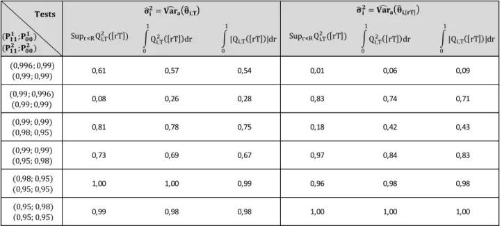
Tables 1 – 3 gather the information relative to the simulation results of

the tests’ empirical size. It is observable that the test size is influenced in

multiple extents, whether it is the sample size, the usage of _σ̂_i2 _{= Var}_̂ a(θ̂i,T)

against _σ̂_i2 _{= Var}_̂

a(θ̂i,⌊rT⌋) or the transition probabilities specified in the DGP.

It seems that the choice of _σ̂_i2_{is quite significant, noticing that}_σ̂ i 2 ₌

Var̂a(θ̂i,⌊rT⌋) is associated with size distortions up to four times the nominal

size for the test introduced by Nicolau (2016), and two times for the

alternative tests. These distortions are mitigated considering _σ̂_i2 _{= Var}̂_a_(θ̂_i,T₎,

with the real size fairly approximating the nominal.

The sample size and DGP also play an important role in the tests’ real

size, with less over-rejection being detected for smaller transition probabilities

(p11; p00) and larger sample sizes. Therefore, one may extrapolate that the

number of state transitions influences the size properties of the given tests,

with these exhibiting less over-rejection the more state transitions verified in

the sample.

Overall, the alternative tests show less over-rejection, comparing with the

(27)

19

Likewise the previous case, the statistical power of the tests is influenced

by the same extents, with addition to the characteristics of the structural

change considered.

Through tables 4 _– 9 it is clear that the sample size and transition

probabilities affect the statistical power in a way that the more state

transitions (larger sample sizes and smaller transition probabilities,_p₁₁ and

p00) the more statistical power.

As it should be expected, the tests evidence more statistical power when

the structural change is in the middle of the sample, comparatively to a more

extreme position (say, in the ₈₀th_{percentile). Such yields the difficulty for the}

tests to detect structural changes in duration of BB markets when these are

verified at the beginning or at the end of the sample.

A rather interesting outcome is obtained when comparing the results for

σ̂i2 = Var̂a(θ̂i,T) against σ̂i2 = Var̂a(θ̂i,⌊rT⌋). It seems that the tests using

σ̂i2 = Var̂a(θ̂i,T) have strictly better power when the structural change is

associated with a decrease in the duration of the cycles, and conversely, the

tests using _σ̂_i2 _{= Var}_̂

a(θ̂i,⌊rT⌋) show more power when there is an increase in

duration of the cycles. This justifies the use of both _σ̂_i2 _{= Var}_̂

a(θ̂i,T) and

σ̂i2 = Var̂a(θ̂i,⌊rT⌋) when applying the structural change tests, since for finite

samples, one is suitable for the detection of increases and the other of

decreases in duration of BB markets.

Comparing the three tests’ statistical power, one verifies that the test

(28)

20

alternatives. Such power may be alarmingly low when working with small

samples sizes and high duration BB markets but reaches admissible values

otherwise, with the tests appearing to be consistent.

In sum_{, the tests’ statistical} properties improve in function of larger

sample sizes and lower transition probabilities which translate in more state

transitions, with the alternative tests showing less problems of size distortion

but also less power in the simulation experiments. The usage of _σ̂_i2 ₌

Var̂a(θ̂i,⌊rT⌋) is justified by its better results in detection of increases in duration

of BB cycles, while _σ̂_i2 _{= Var}_̂

a(θ̂i,T) show better results in detection of

decreases in duration of BB cycles.

5 –

How Are Structural Changes in Duration of Bull

and Bear Markets Connected with the Business Cycle

“[Economists] will have to do their best to incorporate the realities of finance into macroeconomics”

Paul Krugman in New York Times Magazine, 2 September 2009

The links between macroeconomics and finance became an active field

of research especially after the crisis of 2008 that affected economies

worldwide, as economic recessions seem to be accompanied by several

financial disruptions.

Claessens et al. (2009) show that recessions regularly coincide with

(29)

21

moreover, recessions linked with credit crunches and house price busts are

deeper and last longer in comparison with other recessions.

Other authors such as Estrella & Mishkin (1998) and Avouyi-Dovi &

Matheron (2005) had previously tried to relate finance and macroeconomics.

While the former conclude that financial variables such as stock prices have

predictive power over economical recessions in the United States, the latter

show that the stock market cycle and the business cycle verify a significant

concordance in that country, with the start of stock market contractions

preceding contractions in real GDP.

Claessens et al. (2012) addressed the question of “how does the nature

of business cycles vary across different phases of financial cycles?” having

concluded the presence of strong interactions and synchronization among

these cycles, with the financial cycles affecting the duration and strength of

recessions and recoveries in the economy.

The present study aims to be a valid contribution to further

understanding the links between finance and macroeconomics, by exploring

the possible relations of structural changes in duration of BB markets and the

business cycle, a research field never considered to date.

To analyze the connections between structural changes in duration of BB

markets and the business cycle, the statistical tests presented are applied to

adjusted market capitalization stock market indexes of several countries and

the information regarding breakpoints crossed with the peaks and troughs

verified in business cycles and further macroeconomic events. In this sense,

(30)

22

where statistical evidence of structural changes is common among countries

and to perceive how these increases and decreases in duration of BB cycles

are connected with the business cycles.

5.1 –

Data and Methodology

The database comprises adjusted market capitalization stock market

indexes of 37 developed and emerging markets, constructed by Morgan

Stanley Capital International (MSCI) and downloaded from DataStream.

The classification of the market follows three essential criteria: Economic

development, market accessibility and size/liquidity5_{. The adjusted market}

capitalization stock market indexes are derived from the equity universe,

precisely the investable market index. This index is then divided by the size

of the companies with respect to their full market capitalization, resulting in

the large, mid and small cap indexes6_{. For each market (country) considered,}

the structural change tests are applied to the bull and bear markets identified

from the three size indexes.

From the 37 markets considered, 21 are classified as developed and 16

as emerging markets. The developed markets are: Canada and United States

of America from the Americas; Belgium, Denmark, Germany, Finland, France,

Ireland, Israel, Italy, Netherlands, Norway, Portugal, Spain, Sweden,

Switzerland and United Kingdom from Europe and Middle East; Australia,

Hong Kong, Japan and Singapore from the Pacific. The emerging markets

5_See:

www.msci.com/documents/1296102/1330218/MSCI_Market_Classification_Framework+2017.pdf/21f36 0a0-930c-4ca6-9864-d981820dfa0a.

(31)

23

are: Brazil, Chile, Mexico and Peru from the Americas; Hungary, Russia,

South Africa, Turkey, Qatar and United Arab Emirates from Europe, Middle

East and Africa; China, India, Indonesia, Korea, Malaysia and Philippines

from Asia.

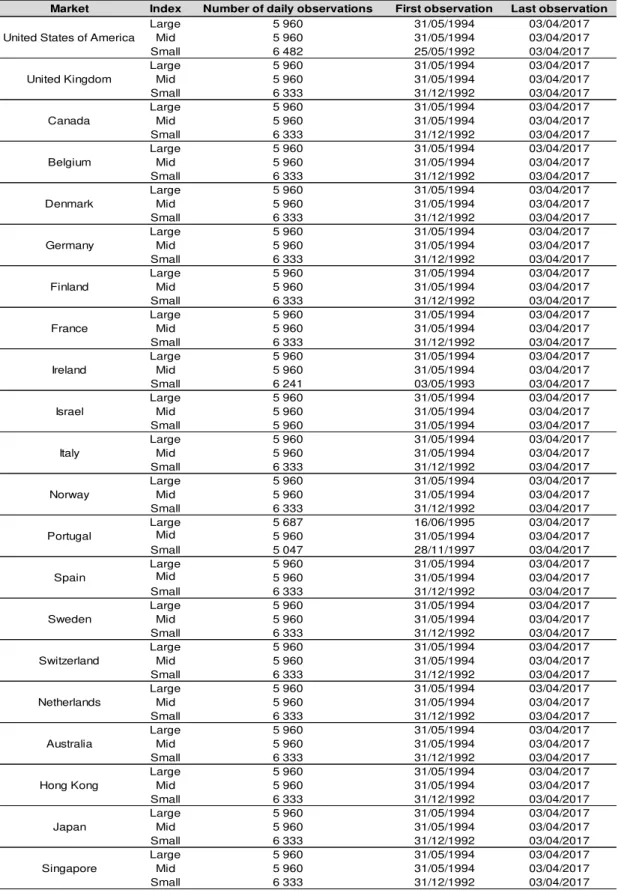
The sample size varies from 3 556 to 6 482 for the daily index prices,

due to restrictions in the availability of its source (DataStream), nevertheless,

the vast majority of the index prices considered have more then 5 900 daily

observations and only for two markets the sample size is less than 5 000. The

last observed period is identical among the elements of the database

considered and it corresponds to the 3rd_{of April 2017 (see tables 10 and 11).}

After the identification of the BB markets inherent to the large, mid and

small cap indexes considered for each country, through the algorithm

suggested by Lunde & Timmerman (2004), the application of the structural

change tests follows. During the course of this analysis, it is admitted that the

estimated dates of breakpoint given by the structural change tests are

consistent. This assumption is supported by Bai (2000) since as specified in

Section 2, the bull and bear markets are assumed to be governed by a

stationary and ergodic first order Markov Chain Process, which has a first

order vector autoregressive representation holding the same asymptotic

proprieties.

The application of the tests is rather simple, yet two remarks arise, the

first one, concerning what start-up values to be used, the choice of _w

(32)

24

strategy where the chosen value is the one that allows for the sample {1, … w}

to have at least two state transitions. Secondly, regarding _σ̂_i2 being the

maximum likelihood estimate of _Var_a_(θ̂_i,T₎ or _Var_a_(θ̂_i,⌊rT⌋₎, both cases are

considered, since as seen previously, the former provides better statistical

power when there is a decrease in duration of bull/bear markets, while the

latter when there is an increase in its duration.

In terms of recognizing statistical evidence of structural changes, the

following set of rules is considered:

a) Since the simulation study performed gave support that the test using

the result in equation (4.1.15) with _σ̂_i2 _{= Var}_̂

a(θ̂i,T) presents few

over-rejection problems and more power than the respective tests that use

(4.2.3) and (4.2.4), then if there is statistical evidence for the rejection

of _H₀ using (4.1.15) at a nominal test size of 0,05, a structural change

associated with a decrease in the cycles is recognized.

b) Since the simulation study performed gave support that the test using

the result in equation (4.1.15) with σ̂_i2 _{= Var}_̂

a(θ̂i,⌊rT⌋) presents

considerable over-rejection but more power than the respective tests

that use (4.2.3) and (4.2.4), a more cautious approach is taken: If there

is statistical evidence for the rejection of _H₀ using (4.1.15) at a nominal

test size of 0,05, and using at least one of the tests associated with

(4.2.3) and (4.2.4), at a nominal test size of 0,10, then a structural

(33)

25

c) Since the tests that use the results in equations (4.2.3) and (4.2.4)

have less over-rejection but also less power than the test that uses

(4.1.15), then if there is statistical evidence for rejecting H0 using

(4.2.3) or (4.2.4) at a nominal test size of 0,05, a structural change

associated with an increase or decrease in the cycles is recognized

(depending on _σ̂_i2_).

It is also admissible that there might be more than one structural change

in the duration of bull or bear markets in a given index. In this sense, after the

application of the tests considering the whole sample, in case there is

statistical evidence of a structural change in a given period, the tests are

applied again using the two subsamples corresponding to the periods before

and after the breakpoint. This simple process allows for the detection of

multiple structural changes.

5.2 _–

Results

The current section focuses on presenting the results obtained from the

application of the structural change tests in duration of BB markets to the

database consisting on large, mid and small cap indexes constructed by

MSCI.

This application led to the results evidenced in figures 1 and 2. A first

analysis to the figures allows the identification of several structural changes in

duration of BB markets in the periods summarized between 1996 and 2015.

(34)

26

some interesting patterns among the different markets. Consider the following

phases regarding the mentioned patterns:

1. 1996 – 2001 (for developed markets) / 1996 – 1998 (for emerging

markets): Period characterized by an increase in the cyclicity of BB

markets, with decreases in the duration of these cycles registered in

several markets.

2. 2002 – 2003 (for developed markets) / 1999 – 2003 (for emerging

markets: Period with several increases in the duration of bull cycles

associated with the given indexes.

3. 2004 – 2008: Numerous structural changes relative to decreases in the

duration of bull cycles (henceforth DDBC) are observed, for both

developed and emerging markets, especially during the period of 2006

– 2007. It is also noticeable that for some developed markets these

structural changes are also accompanied by decreases in duration of

bear markets. Interestingly, the DDBC usually occur first for the

indexes associated with smaller companies and then for the larger.

4. 2009 – 2015: Increases in duration of bear markets are the main

feature perceptible during these periods, with these structural changes

noticeable for several developed and emerging markets.

Given these four phases, it is now intended to compare each one to the

business cycle’s behavior verified in the respective period and further

macroeconomic events7_.

7_{For an extensive chronology of business cycles peaks and troughs presented by the Economic Cycle}

(35)

www.businesscycle.com/ecri-business-cycles/international-business-27

Starting with the first phase perceived, one can observe that the bursting

of the tech bubble, the global recession verified at the beginning of the XXI

century and a gradual increase in the interest rates8_{, which restrains the}

access of credit by companies, match this period of higher volatility with

decreases of both BB markets’ duration.

The increases verified during the second phase are easily explained by

the expansionist period registered in worldwide economies and relatively low

interest rates during that period.

Through the third phase, it is recognizable that the DDBC not only occur

first for the indexes associated with smaller companies, but also seem to

anticipate the recession period confirmed in business cycles worldwide.

These two observations also happen during the first phase, although on a

smaller scale.

To explain the pattern verified between smaller and larger companies,

notice that Kim & Burnie (2002) show that smaller companies are more

vulnerable to adverse changes in economic conditions given their lower

productivity and higher financial leverage. Additionally, Ehrmann (2010)

points that a monetary policy tightening, which leads to restricted access to

credit for companies, is more likely to affect the smaller ones given the higher

amount of collateral they have to pledge and their difficulties to access other

forms of external finance, comparing with larger companies.

cycle-dates-chronologies or see Fushing et al. (2010). For a detailed record of events that made an influence in global macroeconomics see www.businesscycle.com/ecri-about/track-record.

8_See_{www.tradingeconomics.com/country-list/interest-rate}_{for a detailed record of benchmark interest}

(36)

28

Noticing that a monetary policy tightening actually happened during the

third phase, with a progressive increase in interest rates worldwide during the

period before the crisis, one concludes that the structural changes detected

are therefore a combination between the vulnerability of smaller companies

and the conditions verified throughout the pre-crisis period.

To explain the several increases in bear markets duration noticed in the

fourth phase, consider the slowdown in the economic growth and the

industrial slowdown, which provide evidence that although the crisis of 2008

is over, its effects are still present in the economy and in the financial

markets.

One of the most interesting connections detected between structural

changes in duration of BB markets and the business cycle was the fact that

DDBC seem to anticipate periods of economic recession. Beside the use of

visual inspection that allows for such conclusion, it is also desirable to

perceive if there is statistical evidence that supports this statement. To this

end, consider:

Ii(m) = Max {Iismall, Iimedium, Iilarge} (5.2.1)

Where

Iismall = {1 if A(m) _{0 otherwise} (5.2.2)

With _A(m) the event where, for the i-th market, a DDBC in small

companies occurs _m months or less before a peak in the business cycle.

(37)

29

If _I_i_{(m) = 0}, then either no structural changes/economic crisis were

detected during the sample period, or the structural changes did not occur _{s ≤}

m months before the crisis. In order to conduct this statistical application the

first scenario is excluded, in this sense, only the markets where there is

evidence in the sample of at least one DDBC and one economic crisis are

included.

Under the H0 stating that DDBC do not anticipate crisis in business

cycles, _{I_i_(m)} is a sequence of i.i.d random variables with Bernoulli

distribution of parameter _{p ≔ P(I}_i_{(m) = 1)}, which is the probability of at least

one DDBC occurring _m months or less before an economic crisis, for a given

market, with both events independent from each other. Then, the statistic that

allows to test if these structural changes indeed anticipate periods of

economic recession (_H₁₎ is given by:

T(m) = ∑ Ii(m)~Binomial(n, p) n

i=1

(5.2.3)

Where _n is the number of markets in the sample verifying statistical

evidence of DDBC and economic crisis. With T(m) the sum of markets in the

sample which verify at least one DDBC in less than m months before a crisis,

then clearly the greater the _T(m), the greater the likelihood that DDBC

anticipate economic crisis.

(38)

30

p̂ = ∑ ∑ P(x = J ∩ y = L) ∗ [1 − (T − L ∗ m ∗ 250_T 12)

J

]

∞

L=1 k

J=1

(5.2.4)

x being a random variable relative to the total number of DDBC

associated with the small, mid and large indexes of a given market, _y a

random variable relative to the number of economic crisis experienced in that

market during _{1996 − 2017}, and _{k =} T

m∗250₁₂. In this sense, [1 − (

T−L∗m∗250₁₂

T )

J

]

represents the probability of at least one of the _J DDBC found in the size

indexes of a given market anticipates in m months one of its _L economic

crisis. The estimation of P(x = J ∩ y = L) is done using the markets

considered in the sample, by:

P̂(x = J ∩ y = L) = _{#Markets veryfying DDBC and economic crisis (5.2.5)}#Markets verifying J DDBC and L crisis

The number of markets in the database verifying statistical evidence of

DDBC is 26. The following problem arises: The sample size _T is

heterogeneous among markets and among the indexes. This way, the United

Arab Emirates are removed from this analysis since its indexes’ sample size

is reasonably smaller comparing to the other markets. From the 25 left, the

sample sizes are fairly similar, between 5 900 and 6 500 observations, with

the majority verifying _{T = 5}₉₆₀. In this sense, for the present analysis the

(39)

31

To do the confrontation concerning the structural changes and the

economic crisis’ dates, one needs to have the information regarding both. The

former were obtained directly from the application of the statistical tests, while

the latter by considering the dates presented by ECRI9_{if available, and}

through Fushing et al (2010) otherwise10_{. Information regarding the business}

cycles of Hong Kong, Indonesia, Malaysia, Peru and Turkey was not found,

while China evidenced no economic crisis during the period of 1996 – 2017.

In this sense, the number of _n markets considered is 19 (see table 12).

Table 13 presents the results concerning the application of this statistical

test considering two values for _p, one estimated through the method

discussed above and the other an overestimate of _P(I_i_{(m) = 1)}, _{p = 0,5}, more

favorable to the null hypothesis of no connection between DDBC and

economic crisis.

The estimated probabilities inherent to the event in which DDBC occur _m

months or less before an economic crisis, with both events independent are

0,19 and 0,35 for m = 12 and m = 24, respectively. One concludes that for

the 19 markets considered which show statistical evidence of at least one

DDBC and one economic crisis, 14 have at least one DDBC preceding an

economic recession in 12 months. The same number rises to 18 if the

number of months considered is 24.

9_See_{www.businesscycle.com/ecri-business-cycles/international-business-cycle-dates-chronologies}_. 10_{These two sources produce practical results that are relatively similar to each other, yet Fushing et al}

(40)

32

Such result points to a strong statistical evidence that DDBC indeed

anticipate economic crisis in the respective countries. It seems that most

markets considered have at least one DDBC preceding an economic crisis.

The P-Values obtained are significantly small even when using the

overestimate _{p = 0,5}, with the rejection of _H₀_: {DDBC do not anticipate

economic crisis in the business cycle} verified for all the scenarios

considered, for a test size of 0,01.

In summary, the results obtained allow to distinguish several patterns of

structural changes in duration of BB markets, in the countries and indexes

considered. Such structural changes seem to follow certain events occurred

in the macroeconomic cycles, specifically, DDBC seem to anticipate

economic crisis with those structural changes typically being first verified for

smaller companies and then for larger. This way, monitoring the financial

markets with respect to the duration of bull and bear markets may contribute

to the identification and prevention of periods of economic recession.

6 _–

Extensions and Further Research

The application of the structural change tests in duration of BB markets

to the database considered led to a better compression of the relation

between the financial markets, specifically, structural changes in duration of

its BB markets, and the business cycle. As mentioned during this work, such

relation had never been studied to date, which makes this contribution a new

approach in understanding the connections between finance and

(41)

33

area: It would be interesting and relevant, for example, to apply the same

tests to other databases consisting on financial time series and see if the

conclusions of this work still hold, or to detect other possible relations worth of

interest.

Furthermore, since the present work only intends to evidence the

relations between the structural changes in duration of BB markets and the

business cycle, such as DDBC anticipating economic crisis, it is still critical

that one detects promptly these structural changes in order to anticipate

relevant economic events, that is, the financial markets should be into close

inspection for decreases and increases in duration of its BB markets and the

investigation regarding BB markets duration should evolve in direction of

providing methodologies to predict these structural changes.

7 –

Conclusions

This work focused on the study and application of the structural change

test in duration of BB markets proposed by Nicolau (2016) and two alternative

tests computed from the former. These alternatives showed less size

distortions but also less power than the existing test, which yield a great value

in obtaining robust results when applied together with the first test.

The application of the studied tests to a database composed by large,

mid and small cap indexes constructed by MSCI led to the detection of

several relations between the BB markets and the business cycle, as several

breakpoints seemed to be associated with the behavior verified in the

(42)

34

Such relations shed more light in the association between macroeconomics

and finance, an active field of research that gained a new impetus since the

crisis of 2008.

The main breakthrough achieved during this work was the detection of a

relation between DDBC and economic crisis. From inspection, one concludes

that for 14 out of the 19 markets with evidence of both DDBC and economic

crisis during 1996 – 2017, DDBC anticipate at least one economic recession

in 12 months. The same number rises to 18 if an anticipation of 24 months is

considered. Statistically, there is strong evidence that this structural changes

do not happen independently from economic crisis, which provides the

conclusion that DDBC effectively seem to anticipate such macroeconomic

events.

It is suggested that the duration of BB markets should be closely

analyzed in the future, in order to detect possible changes that may be

connected to macroeconomic events, such as the beginning of recession

(43)

35

References

1. Andrews, D. W. K., Ploberger, W. (1994). Tests for Parameter Stability

and Structural Change with Unknown Change Point. Econometrica 62, 1383

– 1414.

2. Avouyi – Dovi, S., Matheron, J. (2005). Interactions between Business

Cycles, Financial Cycles and Monetary Policy: Stylised Facts.BIS Papers22,

273 – 298.

3. Bai, J. (2000). Vector Autoregressive Models with Structural Changes

in Regression Coefficients and in Variance-Covariance Matrices. Annals of

Economics and Finance 1(2), 303 – 339.

4. Basawa, I.V., Rao, P. (1980). Statistical Inferences for Stochastic

Processes: Theory and Methods. Academic Press, London.

5. Bry, G., Boschan, C. (1971). Cyclical Analysis of Time Series: Selected

Procedures and Computed Programs. NBER: New York.

6. Chauvet, M., Potter, S. (2000). Coincident and Leading Indicators of

the Stock Market. Journal of Empirical Finance 7, 87 – 111.

7. Claessens, S., Kose, M. A., Terrones, M. E. (2009). What Happens

During Recessions, Crunches and Busts?.Economic Policy24 (60), 653 –

700.

8. Claessens, S., Kose, M. A., Terrones, M. E. (2012). How do Business

and Financial Cycles Interact?.Journal of International Economics87 (1), 178

Dissertação S TRUCTURAL CHANGES IN DURATION OF BULL AND BEAR MARKETS

M

ESTRADO

ECONOMETRIA

APLICADA

E

PREVISÃO

T

RABALHO

F

INAL DE

M

ESTRADO

Dissertação

S

TRUCTURAL CHANGES IN DURATION OF BULL AND BEAR MARKETS

AND THEIR CONNECTION WITH BUSINESS CYCLES

J

OÃO

A

NTÓNIO

M

ENDES DA

C

RUZ

M

ESTRADO

ECONOMETRIA

APLICADA

E

PREVISÃO

T

RABALHO

F

INAL DE

M

ESTRADO

Dissertação

S

TRUCTURAL CHANGES IN DURATION OF BULL AND BEAR MARKETS

AND THEIR CONNECTION WITH BUSINESS CYCLES

J

OÃO

A

NTÓNIO

M

ENDES DA

C

RUZ

O

:

P

D

J

C

H

C

N

Acknowledgements

Contents

List of Figures

List of Tables

1

–

Introduction

2

–

Preliminary Concepts on BB Markets

3

–

Identification of BB Markets in a Time Series

4

–

Structural Change Tests in Duration of BB Markets

4.1

–

A Revision on Structural Change Tests in Duration of BB

Markets

4.2

–

_–

_–

_–

_–

_–