José Pedro Pontes June 2006
Abstract
This paper models, in game-theoretical terms, the location of two vertically-linked monopolistic firms in a spatial economy formed by a large, high labor cost country and a relatively small, low labor cost country. It is found that the decrease in transport costs shifts firms towards the low production cost country. This process takes two different forms: in labor-intensive industries it leads to spatial fragmentation; in industries with strong input-output relations, agglomerations are conserved, although they shift toward the low labor cost country.
K eyw ords: Location; Intermediate goods; Agglomeration; Com parative advantage.
JE L classification :F10, F12, R30
Author’s affiliation: Instituto Sup erior de Economia e Gestão, Technical University of Lisb on and
Research Unit on Complexity and Economics (UECE)
Address: ISEG, Rua M iguel Lupi, 20, 1249-078 Lisb oa, Portugal
Tel. +351 21 3925916
Fax +351 21 3922808
Em ail<pp [email protected]>
The author wishes to thank André Rocha, Filomena Garcia and Joana Pais for their helpful comments.
1. Introduction
The general decrease in transport costs has caused a shift in productive activity away from countries with large markets towards countries with low labor costs. This process has two different forms depending on the industry involved. In labor-intensive industries (such as the textile industry), with a low intensity of vertical linkages, it leads to spatial fragmentation. In this case, production is located in a low-cost country, while distribution and design are placed close to the majority of the consumers. By contrast, in sectors with strong input-output relations, such as the engineering sectors (aerospace, car, pharmaceuticals, electronics), the agglomerated pattern is maintained, but its location shifts toward a low production cost country. This paper provides a theoretical rationalization for these trends.
in the unit transport costs of the consumer good would shift equilibrium locations toward the point of minimum production costs.
Usually, differences in production costs across locations follow from the fact that the supply of an input is localized, so that the firm not only has to pay the price of the input at its source but also has to transport it over the distance between the firm’s location and the input site. MAYER (2000) explicitly considers this cause of spatial heterogeneity in production costs. However, the localized input is often an intermediate good produced by upstreamfirms. Hence the location of the input is endogenous and interdependent with the location of the consumer good firms. HWANG and MAI (1989) model this interdependence through a two-stage game involving two players that are successive monopolists. In thefirst stage, the upstream and the downstreamfirms simultaneously select locations in an interval whose left boundary is a "port", through which a raw material is imported, and whose right boundary is a "market" in which all consumers locate. In the second stage, the firms set mill prices for the intermediate good and for the consumer good. Subgame perfect equilibrium locations are derived for thefirms, depending on the unit transport costs of the three goods (raw material, intermediate good andfinal good) and on the input-output coefficients. This model suffers from the limitation that the source of the primary input is, by assumption, distinct from the location of the consumers.
differ-ent proportions: upstreamfirms are capital-intensive, while downstreamfirms are labor-intensive. The countries differ in terms of their factor endowments, so that Home is abundant in capital while Foreign is abundant in labor. Besides primary factors, each downstream firm uses a composite intermediate good made by the products of each upstream firm, as in ETHIER (1982).
Apart from the case of autarky, where upstream and downstreamfirms divide evenly between the two countries in order to serve the local consumers, there are two possibilities. If transport costs are intermediate, all thefirms (upstream and downstream) agglomerate in one country, and the downstream industry supplies the other country in manufactured goods through exports. Agglomeration occurs in the Foreign (capital-abundant) country if the transport costs of the intermediate good are low enough in relation to the transport costs of thefinal good. Agglom-eration takes place in the Home (labor-abundant) country if the transport costs of the intermediate good are high enough and the existence of multiple locational equilibria is possible. Finally, if both types of transport cost are low enough, the upstream and downstreamfirms locate in different countries, according to compar-ative advantage, and a fragmented equilibrium emerges. However, AMITI (2005) does not shed enough light on the basic trade-offthatfirms incur between produc-tion costs (which are mainly felt by upstreamfirms) and market access (which is mainly felt by downstreamfirms). The reason is that she focuses on the allocation of each production stage to the country that is abundant in the factor (capital or labor) used more intensively by that production stage.
market size and unit production costs, i.e. the country with the higher number of consumers also has higher production costs. There is a successive monopoly, where an upstream firm uses labor to manufacture an intermediate good. This input is transformed by a downstream firm into afinal good that the firm then sells tofinal consumers. The locational pattern depends on the interaction of unit labor costs, vertical linkages and market access. An exact and detailed definition of locational equilibria in the space of two parameters (intensity of vertical linkages and transport cost) is produced, while the differentials in unit production costs and market size are accounted for through an adequate specification of parameters. The results confirm the position of AMITI (2005) as far as the occurrence of spatial fragmentation in the upstream and downstream stages is concerned, but they differ from her work in other respects, since factor intensity does not play a major role here. In this paper, agglomeration occurs for high transport costs (although in multiple locations), instead of dispersion.
In section 2, a model for the location of vertically-linkedfirms is presented. In section 3, the main conclusions are drawn.
2. The model
2.1. Assumptions
A spatial economy is defined by the following assumptions:
1. There are two countries, labeled Home (H) and Foreign (F). The number of consumers inH is higher than in F: nh > nf. The distance betweenH
2. Each consumer has a linear demand functionq=a−bp, wherepis a delivered price.
3. There are two vertically-related firms. The upstream firm U transforms cu
units of labor into one unit of an intermediate good. The downstreamfirm Dusesαunits of the intermediate good andcdunits of labor to produce one
unit of the final product that is sold to consumers. Firm U is more labor intensive thanfirmD, so that we havecu> cd.
4. The intermediate good has a transport cost τ and the final good has a transport costt. These costs vary in proportion, following the evolution of the general transport infrastructure.
5. Each firm transports and delivers its product to its customers. FirmDsets discriminatory prices ph, pf in each country, while firm U sets a delivered
pricekfor the intermediate good.
6. CountryFis more labor-abundant than countryH, so that the (parametric) wages are such thatwh> wf.
2.2. The structure of the game
The game has two players, namely thefirmsU andD, and three stages:
First stage FirmsU andD simultaneously select locationsxu, xd∈{H, F}.
Second stage Firm U sets a delivered price kfor the intermediate good.
The payoff(profit) functions of thefirms are:
πd(ph, pf, k, xu, xd) = nh(a−bph) [ph−αk−cdwxd−td(xd, H)] +
+nf(a−bpf) [pf−αk−cdwxd−td(xd, F)] (1)
πu(ph, pf, k, xu, xd) = α[nh(a−bph) +nf(a−bpf)]·
·(k−τ d(xd, xu)−cuwxu) (2)
where d(,) is the distance function, and wxd and wxu are the parametric wage
rates in the locations of the downstream and the upstream firms, respectively. In order to concentrate our attention on the parameters that express the in-tensity of vertical linkages (α) and the level of transport costs (t), the following values are assigned to the parameters:
nh = 1.3> nf= 1 (CountryH is larger than CountryF) (3)
cu = 1> cd = 0(Upstream production
is more labor-intensive than downstream production)
wh = 0.3> wf = 0.1(CountryF is
more labor-abundant than countryH)
a = b= 1
With these specifications, 1 and 2 become
πd(ph, pf, k, xu, xd) = 1.3 (1−ph) [ph−αk−td(xd, H)] +
+ (1−pf) [pf−αk−td(xd, F)] (4)
πu(ph, pf, k, xu, xd) = α[1.3 (1−ph) + (1−pf)] [k−td(xd, xu)−wxu]
(5)
The payoffmatrix of the location (first-stage) game can be expressed by
Downstream
H F
Upstream H πu(H, H), πd(H, H) πu(H, F), πd(H, F)
F πu(F, H), πd(F, H) πu(F, F), πd(F, F)
(6)
2.3. Solving the game
In order tofind a subgame perfect equilibrium, each subsequent subgame that begins in a cell of the payoffmatrix 6 is solved by backward induction, yielding profitsπu(α, t)andπd(α, t)that depend only on the intensity of vertical linkages
and on transport costs. The details of these calculations are explained in the Appendix. The profits in thefirst-stage game are:
πd(H, H) = (0.075α+ 0.391 31t−0.25)2+ (7)
+1.3 (0.075α−0.108 70t−0.25)2
πu(H, H) = a
µ
a
µ
0.250 00
a t−
0.575
a −0.172 5
−0.5t+ 1.15
· (8)
·
µ
0.5
a −
0.217 39
a t−0.15
Outcomexu=H, xd=F
πd(H, F) = (0.075α−0.141 31t+ 0.25αt−0.25)2+ (9)
+1.3 (0.075α+ 0.358 70t+ 0.25αt−0.25)2 πu(H, F) = α
µ
0.5
α −0.5t−
0.282 61
α t−0.15
¶ · (10) · µ α µ
0.325
α t−
0.575
α −0.575t−0.172 5
−0.65t+ 1.15
Outcomexu=F, xd=H
πd(F, H) = (0.025α+ 0.391 31t+ 0.25αt−0.25)2+ (11)
+1.3 (0.025α−0.108 70t+ 0.25αt−0.25)2
πu(F, H) = α α
¡0.250 00
α t−0.575α −0.575t−0.057 5
¢
−0.5t+ 1.15
· (12)
·
µ
0.5
α −0.5t−
0.217 39
α t−0.05
Outcomexu=F, xd=F
πd(F, F) = 1.3 (0.025α+ 0.358 70t−0.25)2+ (13)
+ (0.025α−0.141 31t−0.25)2
πu(F, F) = α
µ
α
µ
0.325
α t−
0.575
α −0.057 5
−0.65t+ 1.15
· (14)
·
µ
0.5
α −
0.282 61
α t−0.05
In solving the game, the space of parameters is restricted to those values ofα andt that are low enough, so that the downstreamfirm sells positive amounts of the consumer good in each country. In the Appendix, it is shown that the bounds imposed on the parameters are given by:
0< α < 10 3 ∧
0< t < 39130+250002500(10−α)α if α <0.33229 0< t < 25000(10−α3α+35869)2500 if α >0.33229
(15)
It is easy to check that, for all feasible values of α and t (as defined in 15), the following inequalities hold:
πd(H, H) > πd(H, F) from 7 and 9 (16)
πu(F, F) > πu(H, F) from 14 and 10 (17)
transport cost of the intermediate good and minimizes labor costs, while keeping final demand constant.
Together, inequalities 16 and 17 have two different consequences. The first one is that (H, F) is never a Nash equilibrium of locations. The second one is that the best reply correspondence of firm U is completely determined by sign [πu(H, H)−πu(F, H)], while the best reply correspondence offirmDis also
completely determined bysign [πd(F, H)−πd(F, F)]. The equation system
πu(H, H)−πu(F, H) = 0 (18)
πd(F, H)−πd(F, F) = 0
has a unique feasible solution (in the sense of 15), namely
α = 0.13043 (19)
t = 0.2 (20)
It is simple to check that
πd(F, F) R πd(F, H) iffαR0.13043
πu(H, H) R πu(F, H) ifftR0.2
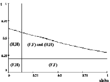
Hence, the regions where a different type of locational Nash equilibrium holds are bounded by 15, 19 and 20. These are plotted in Figure 1.
Figure 1: Location equilibria in(α, t)space.
α and t are both low, the transport cost of the intermediate good is very low. Hence, the upstream and the downstreamfirms choose separate locations(F, H), the former seeking low production costs and the latter seeking high demand. The opposite case is the one where bothαandtare high, so that the transport cost of the intermediate good is high. In this case, thefirms agglomerate and there are multiple equilibria(H, H)and(F, F), as was stressed by FUJITA (1981): locations do not matter as long as thefirms cluster and thus avoid the transport cost of the heavy intermediate good.
of the intermediate good is high in relation to the transport cost of the consumer good. Hence, locations are driven by the minimization of production costs, so that both firms locate in the low labor cost countryF.
3. Concluding remarks
The model presented in the previous section enabled us to explain the trends of the location of vertically-linkedfirms, whenever transport costs are reduced by an improvement in the transportation system. When transport costs are high, firms cluster in the country with the larger market (although agglomeration can
also occur in a peripheral country provided that vertical linkages are high enough). Then, the decrease of transport costs shifts the location of thefirms towards the low-cost country. This process has two different possible forms. If the intensity of vertical linkages is low and the industry is labor-intensive (as in the textile industry), the fall of transport costs leads to fragmentation: production is located in the low-cost country, while the distribution and design are located in the larger market. By contrast, sectors where the intensity of input-output relations is high, such as the engineering sectors (as cars, aerospace, pharmaceuticals, electronics), remain agglomerated, but the location of the cluster shifts towards the low-cost country.
As afirst step, this paper is based on a numerical example. Its generalization is left for further research.
(i) In the case(H, H), the profit functions 4 and 5 become
πd(H, H) = 1.3 (1−ph) (ph−αk) + (1−pf) (pf−αk−t) (21)
πu(H, H) = α[1.3 (1−ph) + (1−pf)] (k−0.3) (22)
Maximizing 21 in relation toph,pf, we obtain the prices of the consumer good:
pf = 0.5t+ 0.5αk+ 0.5 (23)
ph = 0.5αk+ 0.5 (24)
Plugging 23 and 24 into 22 and maximizing the profit function of the upstream firm in relation to the price of the intermediate good, we obtain
k= 0.5
α −
0.217 39
α t+ 0.15 (25)
Substituting 23, 24 and 25 in the profit functions 22 and 21, we obtain the profit functions in terms ofαandt, as given by 8 and 7. The condition of positivity of the outputs sold in the two markets is such that
pf <1⇔t <
2500 (10−3α)
39130 (26)
A necessary condition to ensure that this inequality is met is
α < 10
(ii). In the case(H, F), the profit functions 4 and 5 become
πd(H, F) = 1.3 (1−ph) (ph−αk−t) + (1−pf) (pf−αk) (28)
πu(H, F) = α[1.3 (1−ph) + (1−pf)] (k−t−0.3) (29)
Maximizing 28, the delivered prices of the consumer good are obtained
pf = 0.5αk+ 0.5 (30)
ph = 0.5t+ 0.5αk+ 0.5 (31)
Plugging 30 and 31 into the profit function 28 and maximizing this profit function with relation tok, we obtain the price of the intermediate good
k= 0.5t+0.5
α −
0.28261
α t+ 0.15 (32)
Substituting 32, 30 and 31 into 29 and 28, we obtain the profit functions in terms ofαand tgiven by 9 and 10.
A sufficient condition so that the downstreamfirm sells a positive amount of consumer good in each market in the case(H, F)is that the output sold in market H (the distant market) is positive. Given 31 and 32, this condition means that
ph<1⇔t <
(10−3α) 2500
25000α+ 35869 (33)
A necessary condition so that 33 is fulfilled is
α < 10
(iii) In the case(F, H), the profit functions 4 and 5 become
πd(F, H) = 1.3 (1−ph) (ph−αk) + (1−pf) (pf−αk−t) (35)
πu(F, H) = α[1.3 (1−ph) + (1−pf)] (k−t−0.1) (36)
Maximizing 35 we obtain the prices of the consumer good in each country
pf = 0.5t+ 0.5αk+ 0.5 (37)
ph = 0.5αk+ 0.5 (38)
Plugging 37 and 38 into 36 and maximizing the upstream profit function, the price of the intermediate good is obtained
k= 0.5t+0.5
α −
0.217 39
α t+ 0.05 (39)
Substituting 37, 38 and 39 in the profit functions 35 and 36, we obtain the profit functions in terms ofαandt, as given by 11 and 12.
A sufficient condition so that the output sold in each market is positive is
pf <1⇔t <
2500 (10−α)
39130 + 25000α (40)
A necessary condition so that this inequality is met is
(iv) In the case(F, F), the profit functions 4 and 5 become
πd(F, F) = 1.3 (1−ph) (ph−αk−t) + (1−pf) (pf−αk) (42)
πu(F, F) = α[1.3 (1−ph) + (1−pf)] (k−0.1) (43)
Maximizing 42, wefind the prices of the consumer good
pf = 0.5αk+ 0.5 (44)
ph = 0.5t+ 0.5αk+ 0.5 (45)
Plugging these prices into the profit function 43 and maximizing it in relation tok, we obtain the price of the intermediate good
k= 0.5
α −
0.282 61
α t+ 0.05 (46)
If we substitute 44, 45 and 46 in the profit functions 42 and 43, we obtain these profit functions in terms ofαandt, as given in 13 and 14.
A sufficient condition so that the downstreamfirm sells a positive amount in each country is that
ph<1⇔t <
2500 (10−α)
35870 (47)
A necessary condition so that 47 is fulfilled is
α <10 (48)
firm sells positive outputs in each country is given by
0< α < 10 3 ∧
0< t < 39130+250002500(10−α)α if α <0.33229 0< t < 25000(10−α3α+35869)2500 if α >0.33229
References
AMITI, Mary (2005), "Location of vertically linked industries: agglomeration ver-sus comparative advantage",European Economic Review, 49, pp. 809-832.
ETHIER, Wilfred (1982), "National and international returns to scale in the mod-ern theory of intmod-ernational trade", American Economic Review, 72(3), June, pp. 389-405.
FUJITA, Masahisa (1981), "Location offirms with input transactions", Environ-ment and Planning A, 13, pp. 301-320.
HWANG, Hong and Chao-cheng MAI (1989), "On the optimum location of ver-tically related firms with simultaneous entry", Journal of Regional Science, 29(1), pp. 47-61.