On the time-varying relationship between EMU sovereign spreads and their determinants

Carlos Pestana Barros & Nicolas Peypoch

A Comparative Analysis of Productivity Change in Italian and Portuguese Airports

WP 006/2007/DE _________________________________________________________

António Afonso, Michael G. Arghyrou, George Bagdatoglou and Alexandros Kontonikas

On the time-varying relationship between EMU

sovereign spreads and their determinants

WP 05/2013/DE/UECE _________________________________________________________

De pa rtme nt o f Ec o no mic s

W

P

ISSN Nº 0874-4548

School of Economics and Management

1

On the time-varying relationship between EMU sovereign

spreads and their determinants

António Afonso,

Michael G. Arghyrou,

George Bagdatoglou

and Alexandros Kontonikas

February 2013

Abstract

We use a dynamic multipath general-to-specific algorithm to capture structural instability in the link between euro area sovereign bond yield spreads against Germany and their underlying determinants over the period January 1999 – August 2011. We offer new evidence suggesting a significant heterogeneity across countries, both in terms of the risk factors determining spreads over time as well as in terms of the magnitude of their impact on spreads. Our findings suggest that the relationship between euro area sovereign risk and the underlying fundamentals is strongly time-varying, turning from inactive to active since the onset of the global financial crisis and further intensifying during the sovereign debt crisis. As a general rule, the set of financial and macro spreads’ determinants in the euro area is rather unstable but generally becomes richer and stronger in significance as the crisis evolves. JEL: C22, C52, E43, E62, G12.

Keywords: euro area, crisis, spreads, time-series analysis, time-varying relationship.

*

We are grateful to participants in seminars at the Cardiff Business School, and at the Central Bank of Greece. The opinions expressed herein are those of the authors and do not necessarily reflect those of the ECB or the Eurosystem. $

ISEG/TULisbon – Technical University of Lisbon, Department of Economics; UECE – Research Unit on Complexity and Economics, R. Miguel Lupi 20, 1249-078 Lisbon, Portugal, email: [email protected]. European Central Bank, Directorate General Economics, Kaiserstraße 29, D-60311 Frankfurt am Main, Germany. email: [email protected].



Cardiff Business School, Economics Section, Cardiff University, Colum Drive, Cardiff, CF10 3EU, UK, email: [email protected].

**

Timberlake Consultants, B3 Broomsleigh Business Park, Worsley Bridge Road, London, SE26 5BN, UK, email: [email protected].



2

1. Introduction

The European sovereign debt crisis that started in Greece in the autumn of 2009 and subsequently spread across the whole of the Economic and Monetary Union (EMU) periphery has now entered its fourth year. Since the beginning of the crisis policy makers have taken significant measures both at national as well as at the European level to contain it. These include the implementation of ambitious national adjustment programmes, the creation of the European Financial Stability Fund (EFSF) and of the European Stability Mechanism (ESM), with the purpose of providing financial assistance to countries whose sovereign bonds have come under intense market pressure. Finally, there has been extensive intervention on behalf of the European Central Bank (ECB) at various phases of the crisis in the European sovereign bond markets. These measures, however, have so far achieved only partial success.

Motivated by these developments, a growing empirical literature has attempted to identify the risk factors affecting EMU government bonds yield spreads against Germany, the variable often

3

government bond markets (see e.g. Caceres et al, 2010) as well as a significant response of spreads to changes in credit ratings (see e.g. De Santis, 2012).

The majority of the early studies on the European debt crisis capture the structural instability in the relationship between spreads and their determinants by exogenously imposing on the data break points (typically defined within the period summer 2007 to autumn 2008) and estimating sub-sample regressions differentiating between a pre-crisis and a crisis period (see e.g. Barrios et al., 2009; Arghyrou and Kontonikas, 2012; Caggiano and Greco, 2012). More recent studies have provided evidence that structural instability is not restricted to a simple pre- versus post-crisis differentiation; but rather is a more complex process. Afonso et al. (2012), still working with exogenously imposed breaks, identify two breaks in the process of spreads’ determination, respectively occurring in summer 2007 and spring 2009.

On the other hand, Bernoth and Erdogan (2012) use a semiparametric time-varying coefficients panel data model to examine whether euro area spreads movements are linked to a shift in macroeconomic fundamentals or to increased risk pricing reflected in a stronger market reaction to shifts in the value of the various risk factors. They provide evidence in favour of time-varying slope coefficients for the panel as a whole and show that since the onset of the global financial crisis the market reaction to fiscal imbalances increased considerably. Similar findings are reached by Aß_{mann and Boysen-Hogrefe (2012) who use a time-varying coefficients model to capture changes}

in the weights of spreads’ determinants in the euro area over the period 2001-2011.

By highlighting the continuous nature of structural instability characterising the process of

4

countries and common break points in time for all the countries in the panel.1 It is quite probable, though, that the links between sovereign risk and the various risk factors are activated or deactivated at different points in time across different countries. Thus, an econometric approach that allows for this plausible scenario is likely to provide important country-specific information.

In this paper, we deal with country-specific heterogeneity in an explicit manner based on time-series regressions for ten euro area countries. In line with existing literature, we model spreads on proxies of international financial risk, credit risk and liquidity risk. We implement, however, a novelty to the study of government bond spreads, using a dynamic version of the general-to-specific (GETS) model selection methodology (see Hendry, 2000) allowing us to capture changes in the

statistical significance and size of the coefficients of spreads’ determinants over time. To the best of our knowledge, with the exception of the study by D’Agostino and Ehrmann (2012), our paper is the first to provide information capturing the changing relationship between spreads and their fundamentals on a country-specific basis. D’Agostino and Ehrmann (2012), however model government bond yield spreads against the US and Germany for G7 countries. Therefore, although they provide important insights relating to the French and Italian spread versus Germany, they do not study developments in EMU periphery countries such as Greece, Portugal and Spain, whose role in the European debt crisis has been very prominent. By considering spreads of euro area members versus Germany, we put European developments at the heart of the analysis. Our empirical findings provide new evidence suggesting that there exists significant heterogeneity across countries, both in terms of the risk factors determining spreads over time as well as in terms of the size of their impact on national spreads. As a general rule, the set of financial and macro spreads’ determinants in the euro area is rather unstable but generally becomes richer and stronger in significance as the crisis evolves.

1

In panel estimations of the determinants of euro area spreads, country-specific heterogeneity is typically allowed for

5

The remainder of the paper is structured as follows. Section 2 describes the dataset. Section 3 explains the econometric methodology. Section 4 presents and discusses our empirical findings. Section 5 concludes.

2. Data description

The dependent variable in our econometric analysis is the monthly 10-year government bond yield spread relative to Germany (spr) for ten euro area countries: Austria, Belgium, Finland, France, Greece, Ireland, Italy, Netherlands, Portugal and Spain.2 Our sample covers the period January 1999 - August 2011 (monthly frequency). Following the bulk of existing literature (see e.g. Manganelli and Wolswijk, 2009), we model spreads on the international risk factor as well as country-specific fundamentals, including liquidity risk and credit risk. More specifically, the set of explanatory variables used in our analysis includes the following:

vix denotes the logarithm of the S&P 500 implied stock market volatility index (VIX). In line with previous studies (see e.g. Beber et al., 2009; Afonso et al., 2012) this variable is used to measure the international risk factor.3 We expect a higher value for the international risk factor to cause an increase in government bond spreads.

ba is the bid-ask spread of 10-year government bonds. This variable is extensively used as a proxy for bond market illiquidity (see e.g. Barrios et al., 2009; Favero et al. 2010). A higher value of ba indicates a fall in liquidity leading to an increase in government bond yield spreads.

bal and debt describe the expected (one-year ahead) government budget balance-to-GDP ratio and government debt-to-GDP ratio, respectively, both measured as differentials versus

2

In empirical investigations of euro area spreads, the benchmark ‘risk free’ interest rate, against which spreads are

calculated, is typically approximated by the German government bond yield.

3

The VIX is constructed using call- and put-implied volatilities from the S&P 500 index 30-day options. Implied

volatility measures are forward-looking, as opposed to historical volatility measures that are backward-looking. The

VIX is often called the ‘investor fear gauge’ since it tends to spike during financial market turmoil periods (Whaley,

6

Germany.4 The use of expected, as opposed to historical fiscal data, is in line with a number of recent studies on EMU government bond yield spreads including Attinasi et al. (2009) and Sgherri and Zoli (2009). Fiscal conditions are related to credit quality with an expected fiscal deterioration implying higher credit risk. Hence, a higher (lower) value for the expected government budget balance is expected to reduce (reduce) spreads. By contrast, a higher (lower) lever of expected government debt is positively (negatively) associated with spreads values.

gind is the annual growth rate of industrial production, measured as differential versus Germany. This variable is used as a proxy for the state of business cycle and captures the effect of economic growth on spreads according to which sovereign debt becomes riskier during periods of economic slowdown (see Alesina et al., 1992 and Bernoth et al., 2004). Hence an increase (reduction) in gind should reduce (increase) spreads by improving (worsening) credit worthiness.

Finally, q is the log of the real effective exchange rate. An increase (reduction) in q denotes real exchange rate appreciation (depreciation) expected to increase (reduce) spreads as theoretically justified in the analysis of Arghyrou and Tsoukalas (2011) and empirically documented by Arghyrou and Kontonikas (2012).

[Figures 1, 2]

Figure 1 presents the 10-year euro area government bond yield spreads over our sample period. Before the financial crisis erupted in late 2007 spreads against Germany had stabilised at very low levels despite the fact that macroeconomic fundamentals were deteriorating in many euro area countries, especially in the periphery (see Arghyrou and Kontonikas, 2012). During the credit crisis of 2007-2009 spreads vis-à-vis Germany increased in all euro area economies with German

government bonds operating as a ‘flight-to-quality’ asset. The ‘flight-to-quality’ characteristic of

4

The expected fiscal position data is published bi-annually in the European Commission’s Economic Forecasts. This

semi-annual dataset is transformed into monthly frequency by keeping the expected debt and budget balance

observations constant (equal to the last forecast) for the months between a projection announcement and its subsequent

revisions, when new information becomes available. This is consistent with the idea that before a new projection

7

German bonds is captured in Figure 2, which shows the 10-year German yield together with vix,the proxy of international financial risk. At the climax of the credit crisis, in the aftermath of the Lehman Brothers bankruptcy in September 2008, the VIX increased sharply and at the same time the 10-year German government bond yield plummeted as investors made significant purchases of German bonds.

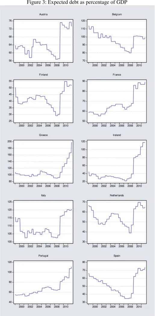
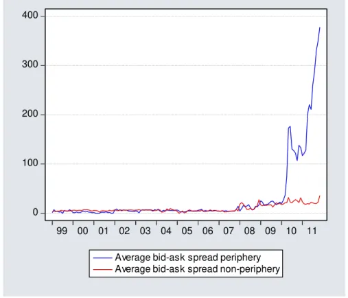
[Figures 3, 4]

Figure 3 plots the expected government debt-to-GDP ratio. This shows a sharp increase in early 2009 as the global credit crisis started to transform into the European sovereign debt crisis. Fiscal deterioration was accompanied by loss of market confidence for the periphery bond markets, credit rating downgrades and liquidity withdrawals, as indicated by the rising periphery bid-ask spreads in Figure 4.

3. Empirical framework

We capture time variation in the link between spreads and their underlying determinants through a dynamic GETS modelling procedure developed and popularised over time by D. Hendry and his co-authors (see e.g. Hendry, 2000). The GETS methodology is a multipath model selection algorithm similar in spirit to Autometrics (see Doornik, 2009), a model selection algorithm embedded in PcGive/OxMetrics (see Hendy and Doornik, 2007).5 The starting point of the searching process is the definition of a general unrestricted model (GUM). This should be formulated on the basis of theory, encompass competing models and provide sufficient information on the process that is being modelled (see Hendry and Krolzig, 2005; Doornik, 2009). The search algorithm proceeds by reducing the GUM towards one or more terminal models, considering in principle the whole model space. Terminal models are located when all variables in a particular search node are statistically significant.

5

Autometrics is the second generation model selection algorithm in OxMetrics following PcGets (Hendry and Krolzig,

8 [Figure 5]

In order to demonstrate how the multipath model selection works, consider for example that the GUM includes four explanatory variables (A, B, C and D) as shown in Figure 5. If all four variables are statistically significant at the 1% level the GUM coincides with the terminal model and the search stops. If, on the other hand, the GUM includes statistically insignificant variables, these are deleted one at the time based on their individual significance. If, for example, only variable A is insignificant, the GUM is reduced to BCD, which itself becomes the basis for another search. If all variables in the GUM are statistically insignificant, the algorithm removes each of them, one at the time, considering four three-variable models: BCD, ACD, ABD and ABC.

The reduction process is repeated at each of these four nodes. For instance, if all three variables are insignificant at node BCD, the algorithm will consider three two-variable models: CD, BD and BC. If statistically insignificant variables are included in these two-variable models the search will continue. For instance, if both variables are insignificant at node CD the algorithm will proceed to two one-variable models: C and D. If at each node all variables are insignificant there would be 16 (=24) potential unique models represented by the solid dots in Figure 5.6 Note that it is possible that the search algorithm will yield more than one terminal models. If an explanatory variable appears in more than one terminal model its impact on the dependent variable is calculated by averaging the slope coefficients of that variable across all terminal models.

In our setup, the GUM is given by the following equation:

1

t t t t

spr   spr_ Xβ (1)

where Xt 





fundamentals, as defined in Section 3, and β is the coefficient vector.7

6

There are 15 unique models with at least one variable and one empty model omitted from Figure 5. Hollow dots

represent duplicated models and can be ignored.

7

Due to the persistent nature of spreads, studies of their determinants typically include lagged spreads in the set of

9

The algorithm is applied dynamically using a 60-month rolling window always starting from the GUM shown in Equation (1). In the absence of structural instability in the relationship between spreads and fundamentals, the algorithm should reach the same terminal model(s) across all different sub-samples. In that case, the set of explanatory variables that the algorithm will identify as statistically significant and the size of their coefficients would not change over time. On the other hand, in the presence of shifts in risk pricing the links between sovereign risk and the underlying risk factors may be activated or deactivated at different points in time across different countries. This would give rise to different terminal models across different rolling estimation windows characterised by different statistically significant explanatory variables and/or different magnitudes for the estimated coefficients.

There are three additional key ingredients in our GETS methodology. First, as suggested by Hendry and Krolzig (2005), we impose theory-consistent sign restrictions on the model space: if a variable is statistically significant but exhibits the ‘wrong’ sign, then it is deleted. Effectively, the sign restrictions impose priors on the model space to ensure that the terminal model conforms to economic theory, at least in terms of coefficient signs. This aims to safeguard against reaching terminal models that reflect data artefacts as opposed to fundamental economic relationships.8 In line with the discussion in Section 3, the theoretically appropriate signs for the explanatory

variables’ coefficients are as follows: vix (+), ba (+), bal (-), debt (+), gind (-), and q (+).

Second, in line with the recommendation of Hendry and Santos (2005), the algorithm automatically detects and corrects for any outlying observations, defined by estimated residuals exceeding 3.5 standard deviations, via impulse dummy variables. Outliers may reflect the impact of

irrespectively of their statistical significance. In our estimations, a constant and the first lag of the spread are always

included in the models.

8

The sign deletion criterion is considered before the individual variable significance criterion, which is ignored if one

10

events which are not captured by our explanatory variables, such as bailout news, or news about country-specific political developments.

Finally, since spreads and the various fundamentals exhibit high persistence, asymptotic inference will tend to over-reject the null hypothesis of no-relationship between them (see e.g. Granger et al., 2001). Therefore we used Monte Carlo simulations to calculate 1% critical values for t-tests that account for the observed persistence in the series.9

4. GETS results

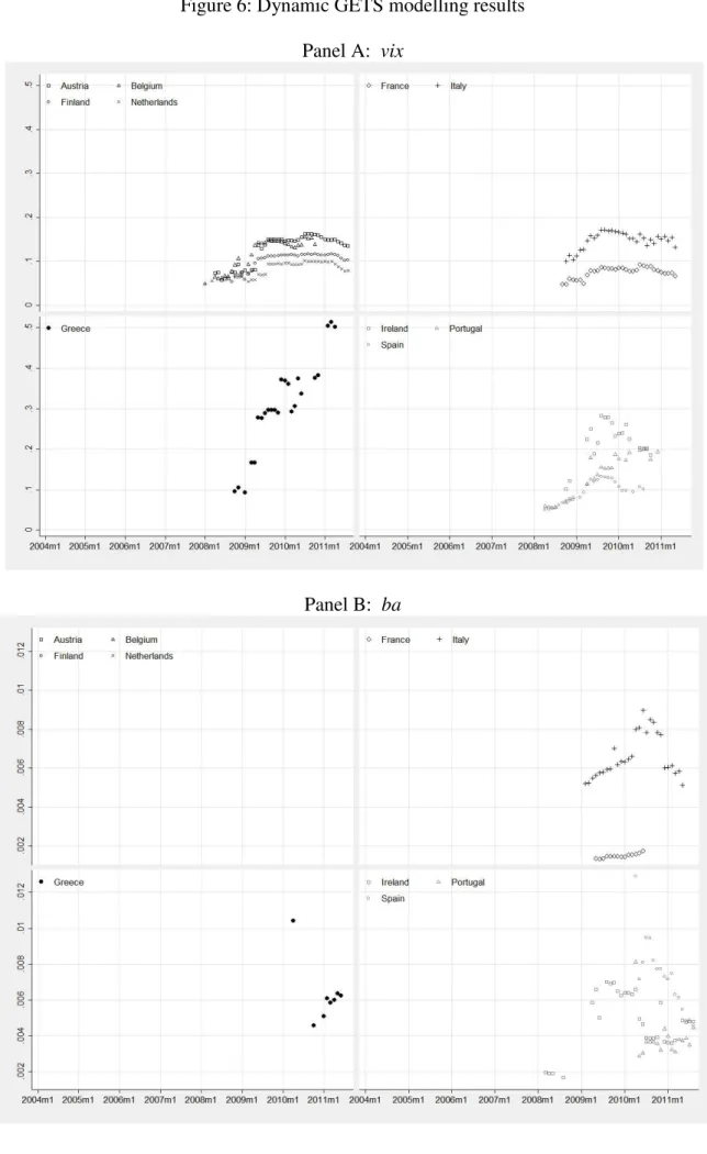
Panels A-E in Figure 6 plot the estimated coefficients of the explanatory variables, obtained from the application of the GETS searching algorithm, when the associated variables enter at least one terminal model at the 1% level of statistical significance.10

[Figure 6]

Figure 6 - Panel A indicates that while prior to the credit crisis the link between spreads and international financial risk was not active, it became strongly active following the intensification of the credit crisis in 2008. Ever since the international risk factor has been a statistically significant determinant of spreads in all sample EMU countries. The degree of exposure of spreads to international financial risk, as indicated by the magnitude of the coefficient of vix, tends to be higher in periphery economies. The peak in the values of the vix coefficients observed in the immediate aftermath of the Lehman Brother event is followed by a stabilisation at lower levels in

9

We generate seven independent AR (1) processes with autoregressive coefficients calibrated to the empirical first

order autocorrelation function parameters of the spreads and the six fundamentals. In turn, a model corresponding to

Equation (1) was estimated using the artificial data for each of the countries in our sample using a sample size equal to

60 observations. We generate 50,000 Monte Carlo iterations and collect the t-statistic of each fundamental’s coefficient

for the null hypothesis of zero effect on the dependent variable. Finally, we calculate the 1% critical value using the

empirical distribution of the relevant t-statistics for each country and regressor (results available upon request).

10

The corresponding graph for the real exchange rate is not shown since overall, with the exception of few instances in

11

all countries. The only exception to this rule is Greece, where the impact of international financial risk on spreads continues to increase until the end of the sample period. Indeed, Greece provides a good example of the information gains obtained from employing the dynamic GETS methodology relative to models not accounting for structural breaks or models with time-varying but homogenous (across countries) slope coefficients, such as the one by Bernoth and Erdogan (2012).

The results presented in Figure 6 - Panel B suggest that liquidity risk has been priced mainly in the periphery EMU countries (Greece, Italy, Ireland, Portugal and Spain) during the sovereign debt crisis period with increasing coefficients over the period 2009 to mid-2010. It is interesting to note that over the same period French bonds also appear to have incorporated an illiquidity premium, which they did not incorporate before or after. Since mid-2010, the coefficient of ba has generally declined in the periphery countries and reverted to zero in the case of France. Once again, Greece is an exception to this rule, with the estimated illiquidity effect increasing towards the end of our sample period. The timing of the reversal in the estimated values of ba approximately matches the creation of the EFSF in May 2010 and the initiation of the Security Markets Programme by the ECB. This indicates that the introduction of a systemic response to the European sovereign debt crisis weakened the relationship between liquidity and sovereign risk. Overall, our findings suggest that, with the exception of Greece, the measures taken at a European level since mid-2010, combined with the reduction in the exposure to international financial risk observed over the same period, have had a moderating impact on spreads.

12

French and Austrian spreads are consistently related to the expected fiscal balance since 2009. Moreover, although markets have been penalising higher expected budget deficits with increasing strength in the case of Portugal, the relationship between spreads and the expected budget balance is not particularly strong in Spain and Ireland.

For Greece and Italy, the expected fiscal balance does not appear to be statistically significant after the end of 2010. Since then, Greek fiscal risk appears to be priced via the expected debt channel (see Figure 6 - Panel D). In particular, the estimated coefficient on the Greek debt has registered a particularly pronounced increase over the last sample year (2011), in line with the increase observed in the value of the vix and ba coefficients for the same country (see Figure 6 - Panels A and B, respectively). For the remaining countries, our findings do not support the existence of a strong link between EMU spreads and the expected debt-to-GDP ratio. Thus, it appears that the credit risk channel mainly operates via the expected budget balance, as opposed to expected debt. Finally, output growth is a statistically significant determinant of spreads only in two EMU periphery economies, Greece and Spain and only during the debt crisis period (see Figure 6 - Panel E).

All in all, in line with previous studies our findings suggest that the relationship between euro area sovereign risk and the underlying fundamentals is strongly time-varying, turning from inactive to active since the onset of the global financial crisis and further intensifying during the sovereign debt crisis.11 Our results are overall in line with those reported by Bernoth and Erdogan (2012) and Aß_{mann and Boysen-Hogrefe (2012) who used a time-varying coefficients panel} approach to capture structural instability in spreads determination within the euro area. The

11

Arghyrou and Kontonikas (2012) argue that the finding of non-pricing or mispricing of related fundamentals prior to

the crisis is supportive of the ‘convergence trading’ hypothesis, according to which investors purchased periphery bonds

in the hope that these economies would converge towards Germany. The increased demand for periphery bonds led to

lower spreads and the expectation of convergence became self-fulfilling, generating profits for bond market investors

13

contribution of our approach is to highlight the additional dimension of country-specific heterogeneity, namely the differentiation of the coefficients’ time variation and impact upon spreads across individual countries. This dimension of intra EMU heterogeneity has not been addressed in previous literature.

4.1 Robustness checks

We tested the robustness of our findings with respect to the specification of the dynamic multipath search algorithm in a number of ways. To save space the results are not reported here but are available upon request. First, we repeated the multipath search using a less tight significance level (5% level). Second, we utilised a longer (72-month) rolling window for the estimations. Third, we did not include outliers in the regression models. Fourth, we conducted recursive, as opposed to rolling windows, estimations. Fifth, we did not impose sign restrictions on the model space. Our benchmark results are overall robust to these sensitivity checks.

5. Conclusions

In this paper we have used a dynamic multipath general-to-specific algorithm in order to capture structural instability in the link between euro area sovereign bond yield spreads against Germany and their underlying determinants over the period January 1999 - August 2011. Following the bulk of existing literature, we modelled spreads on proxies of international financial risk, liquidity risk and credit risk. Our approach allows us to identify country-specific time-variation in the relationship between spreads and fundamentals. Our new evidence suggests that there exists significant heterogeneity across countries, both in terms of the risk factors determining spreads over time as well as in terms of the size of their impact on national spreads.

14

15

References

Acharya, V.V., Drechsler, I., Schnabl, P. (2011). “A Pyrrhic victory? – Bank bailouts and sovereign

credit risk”. NBER Working Paper 17136.

Afonso, A., Arghyrou, M.G., Kontonikas, A. (2012). “The determinants of sovereign bond yield

spreads in the EMU”. University of Glasgow, Adam Smith Business School, Discussion Paper

2012-14.

Arghyrou, M.G., Tsoukalas, J. (2011). “The Greek debt crisis: Likely causes, mechanics and

outcomes”. The World Economy,34, 173-191.

Arghyrou, M.G., Kontonikas, A. (2012). “The EMU sovereign debt crisis: Fundamentals,

expectations and contagion”. Journal of International Financial Markets, Institutions and

Money, 22, 658-677.

Alesina, A., De Broeck, M., Prati, A., Tabellini, G. (1992), “Default risk on government debt in

OECD countries”. Economic Policy, 15, 427-451.

Aß_{mann, C., Boyesen-}Hogrefe, J. (2012). “Determinants of government bond spreads in the euro area: in

good times as in bad”. Empirica, 39, 341-356. Attinasi, M-G., Checherita, C., Nickel, C. (2009).

“What explains the surge in euro area sovereign spreads during the financial crisis of 2007

-09?”. ECB Working Paper 1131.

Barrios, S., Iversen, P., Lewandowska, M., Setzer, R. (2009). “Determinants of intra-euro-area

government bond spreads during the financial crisis”. European Commission, Economic Papers

388.

Beber, A., Brandt, M., Kavajecz, K. (2009). “Flight-to-quality or flight-to-liquidity? Evidence from the euro-area bond market”. Review of Financial Studies, 22, 925-957.

Bernoth, K., von Hagen, J., Schuknecht, L. (2004). “Sovereign risk premia in the European

government bond market”. ECB Working Paper 369.

Bernoth, K., Erdogan, B. (2012). “Sovereign bond yield spreads: A time-varying coefficient

16

Caceres, C., Guzzo, V., Segoviano, M., (2010), “Sovereign spreads: Global risk aversion, contagion

or fundamentals?”. IMF Working Paper 10/120.

Caggiano, G., Greco, L. (2012). “Fiscal and financial determinants of Eurozone sovereign spreads”.

Economics Letters, 117, 774-776.

D’Agostino, A., Ehrmann, M., (2012). “The pricing of G7 sovereign bond spreads – the times they are a-changin”, MPRA Paper No 40604.

De Grauwe, P., Ji, Y. (2012). “Mispricing of sovereign risk and macroeconomic stability in the

eurozone”. Journal of Common Market Studies, 50, 866-880.

De Santis, R. (2012). “The euro area sovereign debt crisis: Safe haven, credit rating agencies and

the spread of the fever from Greece, Ireland and Portugal”. ECB Working Paper 1419.

Doornik, J.A., (2009). “Autometrics”. In J. L. Castle and N. Shephard (Eds), The Methodology and

Practice of Econometrics, 88–21. Oxford: Oxford University Press.

Favero, C.A., Missale, A. (2011). “Sovereign spreads in the euro area. Which prospects for a

eurobond?”. CEPR Discussion Paper No. 8637.

Favero, C., Pagano, M., von Thadden, E.-L. (2010). “How does liquidity affect government bond

yields?”. Journal of Financial and Quantitative Analysis, 45, 107-134

Gerlach, S., Schulz, A., Wolff, G. (2010). “Banking and sovereign risk in the euro-area”. CEPR Discussion Paper No. 7833.

Granger, C.W., Hyung, N., Jeon, Y. (2001). “Spurious regressions with stationary series”. Applied Economics, 33, 899-904.

Hendry, D., Krolzig, H. (2001). “Automatic econometric model selection”. London: Timberlake

Consultants Press.

17

Hendry, D., Krolzig, H. (2004). “Sub-sample model selection procedures in general-to specific

modelling”. In R. Becker and S. Hurn (Eds.), Contemporary Issues in Economics and

Econometrics: Theory and Application, 53–74. Cheltenham: Edward Elgar.

Hendry, D., Krolzig, H. (2005). “The properties of automatic Gets modelling”. Economic Journal, 115, 32-61.

Hendry, D., Santos, C. (2005). “Regression models with data-based indicator variables”. Oxford Bulletin of Economics and Statistics, 67, 571-595.

Hendry, D. (2000). “Econometrics: Alchemy or Science?”. Oxford: Oxford University Press.

Manganelli, S., Wolswijk, G. (2009). “What drives spreads in the euro-area government bond

market?”. Economic Policy, 24, 191-240.

Newey, W., West, K., 1987. A simple positive semi-definite, heteroskedasticity and autocorrelation consistent covariance matrix. Econometrica 55, 703-70.

Schuknecht, L., von Hagen, J., Wolswijk, G. (2010). “Government bond risk premiums in the EU

revisited: The Impact of the financial crisis”. ECB Working Paper 1152.

Sgherri, S., Zoli, E. (2009). “Euro area sovereign risk during the crisis”. IMF Working Paper

09/222.

18

Figure 1: 10-year government bond yield spreads

0.0 0.5 1.0 1.5

2000 2002 2004 2006 2008 2010 Austria

0 1 2 3

2000 2002 2004 2006 2008 2010 Belgium -0.2 0.0 0.2 0.4 0.6 0.8 1.0

2000 2002 2004 2006 2008 2010 Finland 0.0 0.4 0.8 1.2 1.6

2000 2002 2004 2006 2008 2010 France 0 5 10 15 20

2000 2002 2004 2006 2008 2010 Greece -2 0 2 4 6 8 10

2000 2002 2004 2006 2008 2010 Ireland 0 1 2 3 4 5 6

2000 2002 2004 2006 2008 2010 Italy -.2 .0 .2 .4 .6 .8

2000 2002 2004 2006 2008 2010 Netherlands 0 2 4 6 8 10 12

2000 2002 2004 2006 2008 2010 Portugal 0 1 2 3 4 5

19

Figure 2: German 10-year government bond yield and VIX

1 2 3 4 5 6

2.0 2.5 3.0 3.5 4.0 4.5

99 00 01 02 03 04 05 06 07 08 09 10 11

20

Figure 3: Expected debt as percentage of GDP

56 60 64 68 72 76

2000 2002 2004 2006 2008 2010 Austria 70 80 90 100 110 120

2000 2002 2004 2006 2008 2010 Belgium 25 30 35 40 45 50 55

2000 2002 2004 2006 2008 2010 Finland 50 60 70 80 90

2000 2002 2004 2006 2008 2010 France 80 100 120 140 160 180 200

2000 2002 2004 2006 2008 2010 Greece 20 40 60 80 100 120

2000 2002 2004 2006 2008 2010 Ireland 100 105 110 115 120 125

2000 2002 2004 2006 2008 2010 Italy 30 40 50 60 70

2000 2002 2004 2006 2008 2010 Netherlands 40 60 80 100 120

2000 2002 2004 2006 2008 2010 Portugal 30 40 50 60 70 80

21

Figure 4: Average bid-ask spread in periphery and non-periphery countries

Note: Periphery countries include Greece, Ireland, Portugal and Spain. Non-periphery countries include Austria, Belgium, Finland, France, Italy and the Netherlands.

Figure 5: Multipath model space

Note: Figure 5 has been reproduced from Doornik (2009). It shows all unique models starting from a general unrestricted model (GUM) with variables ABCD.

0 100 200 300 400

99 00 01 02 03 04 05 06 07 08 09 10 11

Average bid-ask spread periphery Average bid-ask spread non-periphery

ACD

ABC

AB ABD

ABCD

AC AD BC BD

A BCD

CD D

C

22

Figure 6: Dynamic GETS modelling results Panel A: vix

23 Panel C: bal

24 Panel E: gind