Implied probability density
functions:
Estimation using hypergeometric,
spline and lognormal functions
A thesis presented
by
André Duarte dos Santos
to
The Department of Finance
in partial ful…llment of the requirements
for the degree of
Master of Science in Finance
in the subject of
Finance
UNIVERSIDADE TÉCNICA DE LISBOA
Supervisor: Prof. Doutor João Guerra
Dissertation Committee:
Prof. Doutora Teresa Garcia, Chairman
Prof. Doutor Jorge Barros Luís
Prof. Doutor João guerra
Abstract
This thesis examines the stability and accuracy of three di¤erent methods to estimate Risk-Neutral Density functions (RNDs) using European options. These methods are the Double-Lognormal Function (DLN), the Smoothed Implied Volatility Smile (SML) and the Density Functional Based on Con‡uent Hypergeometric function (DFCH).
These methodologies were used to obtain the RNDs from the option prices with the underlying USDBRL (price of US dollars in terms of Brazilian reals) for di¤erent maturities (1, 3 and 6 months), and then tested in order to analyze which method best …ts a simulated "true" world as estimated through the Heston model (accuracy measure) and which model has a better performance in terms of stability.
We observed that in the majority of the cases the SML outperformed the DLN and DFCH in capturing the "true" implied skewness. The DFCH and DLN methods were better than the SML model at estimating the "true" Kurtosis. However, due to the higher sensitivity of the skewness and kurtosis measures to the tails of the distribution (all the information outside the available strike prices is extrapolated and the probability masses outside this range can have in…nite forms) we also compared the tested models using the root mean integrated squared error (RMISE) which is less sensitive to the tails of the distribution. We observed that using the RMISE criteria, the DFCH outperformed the other methods as a better estimator of the "true" RND.
Acknowledgement
First of all, I would like to thank my supervisor, Professor João Guerra, for all the support and interesting discussions during the preparation of this thesis.
I would like also to acknowledge to my dear friends João Pedro, Pedro Gonçalves and Tiago Neves for their useful advice and help in the thesis preparation.
All my friends for their friendship and encouraging support.
Contents
1 Introduction 1
2 Standard option pricing and extraction of RND 4
2.1 Option pricing and Black & Scholes model . . . 4
2.2 Implied Volatility and limitations of the Black & Scholes model . . . 7
2.3 Relation between option prices and the extraction of RNDs . . . 8
3 RND estimation - Alternative methods 12 3.1 Structural Models . . . 13
3.1.1 Jump Di¤usion Model . . . 13
3.1.2 RND estimation using a model based on stochastic volatility - He-ston Model . . . 14
3.2 Non-Structural Models . . . 15
3.2.1 Parametric models . . . 15
3.2.2 Non-parametric models . . . 23
4 Accuracy and Stability analysis of the tested PDF estimation methods 27 4.1 Data . . . 27
4.2 Testing PDF estimation techniques using Monte Carlo approach . . . 29
4.3 Statistics used in comparison of di¤erent techniques . . . 34
4.4.2 Density Functional Based on Con‡uent Hypergeometric Function 39
4.4.3 Smoothed Implied Volatility Smile . . . 40
5 Comparison of di¤erent methods using the Cooper scenarios 42 5.1 Analysis using mean, standard deviation, skewness and kurtosis . . . 43
5.1.1 Accuracy . . . 43
5.1.2 Stability . . . 48
5.2 Analysis using RMISE . . . 51
5.2.1 SML with v weighting or with equal weighting . . . 52
5.2.2 Best Performance of the DFCH and MLN as the estimators of the "true"RND . . . 53
5.2.3 Comparing DFCH with MLN accuracy . . . 53
5.2.4 Stability . . . 54
5.3 Comparison of our results with other studies . . . 54
6 Comparison of di¤erent methods using USDBRL Heston calibrated pa-rameters 56 6.1 Analysis using mean, standard deviation, skewness and kurtosis . . . 57
6.1.1 Accuracy . . . 57
6.1.2 Stability . . . 62
6.2 Analysis using RMISE . . . 66
6.2.1 Best Performance of the DFCH and MLN model . . . 69
6.2.2 Stability . . . 69
7 Information contained in the option implied risk-neutral probability density function 70 7.1 Analyzing changes of implied pdf summary statistics over time . . . 70
7.1.1 Comparing MLN, SML and DFCH . . . 70
8 Conclusion 86
9 Further research 90
10 Appendix A 92
10.1 Geometric Brownian motion . . . 92
10.2 Itô’s Lemma . . . 93
10.3 Stochastic Volatility . . . 96
10.4 Mixture of hypergeometric functions . . . 99
11 Appendix B 106 12 Matlab Codes 119 12.1 Heston model Codes . . . 119
12.1.1 Generate Cooper Scenarios . . . 119
12.1.2 USDBRL Heston parameters . . . 127
12.2 Hypergeometric model codes . . . 133
12.2.1 DFCH Monte Carlo simulations for USDBRL Heston Scenarios . 133 12.2.2 DFCH USDBRL parameters . . . 139
12.3 Spline model codes . . . 146
12.3.1 SML USDBRL parameters . . . 146
12.4 MLN model codes . . . 150
List of Figures
2-1 Volatility Smile curve at 29/08/2008 calculated using USDBRL options
prices that expire in one month . . . 8
4-1 Implied RND under aternative values for the correlation parameter . . . 31
5-1 Best method in terms of accuracy for each combination of scenario and
maturity . . . 44
5-2 Summary statistics obtained for Heston model (true density) and mean of summary statistics obtained for DFCH, MLN and SML methods. The
results estimated for the SML method were processed with v weighting
and with the smoothing parameter that minimizes RMISE. . . 45
5-3 Di¤erence between the "true" and the mean summary statistics in per-centange of the "true" statistics.The results estimated for the SML method
were processed withv weighting and with the smoothing parameter that
minimizes RMISE. . . 46
5-4 The most stable method for each combination of scenario and maturity . 49
5-5 Standard Deviation of the summary statistics for the SML, MLN and
DFCH methods . . . 50
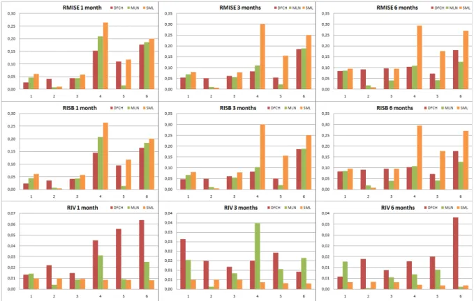
5-6 Values for RMISE, RISB and RIV. The results shown for the SML method
were processed with v weighting and the smoothing parameter that
minimizes RMISE . . . 52
6-2 Best method in terms of accuracy for the high volatility dates . . . 58
6-3 Low Volatility Dates: Di¤erence between the "true" and the mean sum-mary statistics in percentange of the "true" statistics: (true-mean)/true. The results for the SML method were processed withv weighting and with the smoothing parameter that minimizes RMISE. . . 59
6-4 High Volatility Dates: Di¤erence between the "true" and the mean sum-mary statistics in percentange of the "true" statistics: (true-mean)/true. The results for the SML method were processed withv weighting and with the smoothing parameter that minimizes RMISE. . . 60
6-5 The most stable method for the low volatility dates . . . 62
6-6 The most stable method for the high volatility dates . . . 63
6-7 Low Volatility Dates: Standard Deviation of the summary statistics for the SML, MLN and DFCH methods . . . 64
6-8 High Volatility Dates: Standard Deviation of the summary statistics for the SML, MLN and DFCH methods . . . 65
6-9 Low Volatility Dates: Values for RMISE, RISB and RIV. The SML results were processed with v weighting and the smoothing parameter that minimizes RMISE . . . 67
6-10 High Volatility Dates: Values for RMISE, RISB and RIV. The SML results were processed with v weighting and the smoothing parameter that minimizes RMISE . . . 68
7-1 Evolution of one month to maturity expected value . . . 71
7-2 Evolution of one month to maturity standard deviation . . . 72
7-3 Evolution of one month to maturity skewness . . . 73
7-4 Evolution of six months to maturity skewness . . . 73
7-5 Evolution of one month to maturity Pearson mode . . . 74
7-6 Evolution of one month to maturity Pearson median . . . 75
7-8 Evolution of 6 months to maturity Kurtosis . . . 76
7-9 3 months RNDs at 28th November 2008 estimated through DFCH, MLN and SML methods using USDBRL FX options . . . 77
7-10 Evolution of implied expected value estimated through DFCH method . . 81
7-11 Evolution of implied standard deviation estimated through DFCH method 82 7-12 Evolution of implied skewness estimated through DFCH method . . . 82
7-13 Evolution of implied Pearson mode estimated through DFCH method . . 83
7-14 Evolution of implied Pearson median estimated through DFCH method . 83 7-15 Evolution IQR 1 month . . . 84
7-16 Evolution IQR 3 months . . . 84
7-17 Evolution IQR 6 months . . . 85
7-18 Evolution of implied kurtosis estimated through DFCH method . . . 85
11-1 Summary Statistics obtained for DFCH and MLN methods . . . 106
11-2 Summary Statistics obtained for SML method under 4 scenes: with or without v weighting and for each weighting approach using a smoothing parameter that minimizes RMISE or a smoothing parameter with a value of 0,9. . . 107
11-3 Di¤erence between the "true" and mean summary statistics in percentage of the "true" statistics for the DFCH and MLN methods. . . 108
11-7 RMISE, RISB and RIV for DFCH and MLN methods. . . 112
11-8 RMISE, RISB and RIV for the SML method under 4 scenes: with or without v weighting and for each weighting approach using a smoothing parameter that minimizes RMISE or a smoothing parameter with a value of 0,9. . . 113
11-9 Heston model parameters obtained through calibration between June 2006 and February 2010 . . . 114
11-10Brazil GDP . . . 115
11-11USD GDP . . . 116
11-12FED Funds target rate . . . 117
Chapter 1
Introduction
It is accepted by market participants that the prices of …nancial derivatives provide in-formation about future expectations of the underlying asset prices, especially forwards, futures and options. Forwards and futures only give us the expected value for the un-derlying asset under the assumptions of risk neutrality, which makes using cross-sections of observed option prices more attractive because they allow estimation of an implied probability density function.
For market agents, the attractiveness of using an implied probability density function relies on being able to attribute probabilities to a range of future events, using market perceptions at a certain time. Several decision makers and analysts use this informa-tion source when analyzing market sentiment, uncertainty and extreme event scenarios, especially for interest rates and exchange rates.
the robustness of these estimates and their information power.
In this thesis we compare three methods of extracting RNDs from USDBRL Euro-pean type exchange rate options. These methods are the Double-Lognormal Function, the Smoothed Implied Volatility Smile and the Density Functional Based on Con‡uent Hypergeometric function. We test the stability of the estimated RNDs and their robust-ness as regards small errors by randomly perturbing option prices by half of the quotation of the tick size as in Bliss and Panigirtzoglou (2002) before re-estimating the RNDs and their accuracy by experimenting their capacity to recover the "true" RNDs. The "true" probability density function (pdf) was estimated using the method developed in Cooper (1999), who generated pseudo prices from Heston’s stochastic volatility model, and then compared the performance of the di¤erent methods using Monte Carlo simulations in or-der to obtain RNDs, whereby the input was the option prices calculated by these pseudo prices.
The remainder of this thesis is organized into seven chapters. Chapter Two gives a brief explanation of option pricing and a presentation of the Black and Scholes model and its theoretical background. We also describe the limitations of this model and its failure to capture the volatility smile contributions, due to the di¤erence between the lognormal distribution mapped by the model and the real distribution of the underlying asset prices of the market (the di¤erence between the theoretical B&S prices and the market prices). In this chapter, we also describe how option prices can provide information about implied probabilities given by market participants to future events and its use as an instrument to extract probability density functions of future prices using the formula proposed in Breeden and Litzenberger (1978).
estimation of a RND without describing any evolving process for the price or volatility of the underlying asset. The non-structural approaches can be divided into three subcat-egories: parametric (propose a form for the RND without assuming any price dynamics for the underlying asset), semi-parametric (suggest an approximation of the true RND) and non-parametric models (do not propose an explicit form for the RND).
Chapter Four explains the technical details of the strategies used in this thesis in order to estimate the RNDs and describe the measures used to evaluate the performance of the three models tested (MLN, SML and DFCH) in terms of accuracy and stability.
Chapter 2
Standard option pricing and
extraction of RND
2.1
Option pricing and Black & Scholes model
Let us begin by introducing two elementary types of options. A European call option gives the buyer the right to buy the underlying asset for a certain price (strike price) at a certain date (maturity), whereas a European put option gives the buyer the right to sell the underlying asset for a certain price at a certain date. American options can be exercised at any time until expiration. In this thesis we will focus on European options. At maturity, the holder of the option only exercises it if he has a positive payo¤ (if the price of the underlying asset is above the exercise price for the call option or if the price of the underlying asset is below the exercise price for the put option).
Assuming that there are no transaction costs, we can represent the payo¤ of an European option at maturity through the following formulas (call option and put option),
where X is the exercise price of the option, ST is the price of the underlying asset at
C(ST; T; X) = max(ST X; 0) (2.1)
P(ST; T; X) = max(X ST; 0) (2.2)
Intuitively, it can be inferred that the price of a call option re‡ects the ability to exercise the option when it brings a pro…t. This depends on the probability of the price of the underlying asset being greater than the strike price.
The widely used Black and Scholes model [Black and Scholes (1973)] for option pricing assumes that the underlying asset price has a lognormal distribution and evolves until reaching maturity in line with a geometric Brownian motion (GBM) stochastic process, with a constant expected return and a constant volatility:
dSt = St dt+St dWt (2.3)
where St is the price of the underlying asset at time t, dSt denotes instantaneous price
change, is the expected return, is the standard deviation of the price process anddW
are increments from a Brownian motion process. The parameters and are assumed
to be constant.
Besides constant volatility during the term of the option, the B&S model also assumes the same volatility across the whole range of strike prices.
Itô’s Lemma states that an asset whose value depends on St and t has dynamics
de…ned by the following stochastic di¤erential equation:
df(St; t) =
1 2
d2f dS2
t
2
t +
df
dSt t
+df
dt dt+
df dSt
tdWt (2.4)
Considering Itô’s Lemma (see appendix A) and applying it to equation (2.3) results in
Sthaving a lognormal distribution andlog(St) N( ; )where = log(S0) + ( 12 2)t
and = 2t, which means that the underlying asset price has a lognormal distribution
and the underlying returns are normally distributed.
of units (df
dS) of the underlying asset, we can apply the partial di¤erential equation (2.4)
to this portfolio getting the Black and Scholes partial di¤erential equation (see Jondeau et al. (2006)):
1 2
d2f dS2
t
St2 2+ df
dSt
Str+
df
dt rf = 0 (2.5)
The value of the option depends on r (risk free rate), and the boundary condition
of the option contract in equations (2.1) and (2.2), respectively for calls and puts. Solving the PDE in equation (2.5), in accordance with the boundary conditions, results in the Black and Scholes Pricing formula (call and put price):
C(S;t) = SN(d1)-Xe r(T t)N(d2); S > 0; t2[0;T] (2.6)
P(S;t) = Xe r(T t)N( d
2) SN( d1); S > 0; t2[0;T] (2.7)
with
d1 =
ln(XS) + (r+ 12 2)(T t)
p
(T t) (2.8)
and
d2 =
ln(S
X) + (r
1 2
2)(T t) p
(T t) (2.9)
We can observe that the parameter is not in equation (2.5), which means that the
expected return does not appear in the B&S formula and consequently the value of the option does not depend on the investors’ risk preferences (the solution of the equation is the same regardless of the risk premium required by each investor). In fact, instead
of , equation (2.5) hasr, which is the risk free rate (assumption that investors are risk
does not depend on the change of the stock price.
2.2
Implied Volatility and limitations of the Black &
Scholes model
The Black & Scholes model assumes that the price of the underlying asset follows a stochastic model with constant expected return and constant volatility. The …nal as-sumptions made by Black and Scholes’ argument rely on the fact that if the future prices of the underlying asset are lognormally distributed, an option can be dynamically hedged using the underlying asset in order to build a portfolio that depends exclusively on the risk free rate.
However, in the real world we do not know the distribution of the prices in the future (traders do not have full knowledge of probabilities for future events) and dynamic hedging implies continuous trading (transaction cost problem, liquidity restrictions and not possible in practice).
The parameter regarding the instantaneous volatility in the underlying asset’s return ( ) is not known. However, it can be estimated inverting Black and Scholes’ formula in
terms of (implied volatility) and then using market prices of options as inputs. The
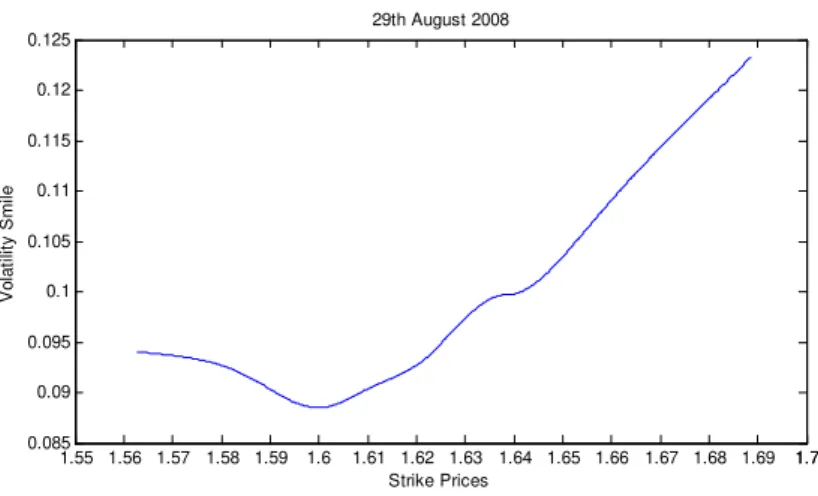
investors observe that the implied volatility calculated for each strike price is di¤erent, and that the implied volatilities are di¤erent across maturities (a volatility curve changes with maturity), which is not consistent with the Black and Scholes lognormal assumptions that de…ne volatility as being constant across the whole range of strike prices and matu-rities. Implied volatilities observed in the market are a convex function of strike prices (usually out-of-the money and in-the-money options have higher volatility compared with at-the-money options), which creates the well known phenomenon called volatility smile.
1.55 1.56 1.57 1.58 1.59 1.6 1.61 1.62 1.63 1.64 1.65 1.66 1.67 1.68 1.69 1.71.7 0.085
0.09 0.095 0.1 0.105 0.11 0.115 0.12 0.125
Strike Prices
V
o
la
tilit
y
S
mile
29th August 2008
Figure 2-1: Volatility Smile curve at 29/08/2008 calculated using USDBRL options prices that expire in one month
which results in fatter tails of the true probability density function (pdf) when compared with a lognormal pdf. This indicates that the investors attribute higher probabilities to extreme events and that there is a gap between the true market RND and the Black and Scholes lognormal RND. In fact, higher volatilities for strike prices deep out-of-the-money make it more likely that future prices will be very di¤erent from current market values. This in turn increases the probability of these option prices being in-the-money in the future and leads to more expensive prices for deep out-of-the-money options, when compared to prices calculated through the B&S model.
2.3
Relation between option prices and the
extrac-tion of RNDs
This relation between probabilities and the price of a contingent claim1 was initially
proposed in Arrow (1964) 2 who applied a contingent claim model to the securities
market. It was shown that the prices of an elementary claim (Arrow-Debreu security)3
are proportional to the risk-neutral probabilities attached to each of the states.
This Arrow-Debreu security has an important information value and can be replicated
with a combination of European call options, called butter‡y spread, which consists of a
long position in two calls with strikes (X M) and (X+ M) and a short position in
two calls with strike (X) , where M > 0.
Breeden and Litzenberger (1978) applied the developments by Arrow and Debreu and
used a state contingent claim in the form of a butter‡y spread to show that the second
partial derivative of a call option pricing function with respect to the strike prices yields
the discounted RND (f(ST) e rT).
In fact, a butter‡y spread centered on X implies a payo¤ of M if the price of the
underlying asset at maturity T is equal toX (see Example 1).
Example 1 (Breeden and Litzenberger (1978))
Portfolio composed by [c(0; T) c(1; T)] [c(1; T) c(2; T)]withT =M aturity will
pay 1 unit if the state M(T) = 1 (butter‡y spread centered in 1)
1a claim that can be made when a speci…c outcome occurs.
2who introduced uncertainty into the notion of competitive equilibrium and Pareto Optimality (Pareto equilibrium refers to a situation in economy where it’s impossible to bene…t an economic agent without harming another agent).
Aggregate Wealth c(0; T) c(1; T) c(2; T)
M(T) = 0 0 0 0
M(T) = 1 1 0 0
M(T) = 2 2 1 0
M(T) = 3 3 2 1
. . . .
M(T) = N N N 1 N 2
Aggregate Wealth c(X M; T) c(X; T) c(X+ M; T) Payo¤ of Butter‡y Spread
M(T) =X M 0 0 0 0
M(T) = X M 0 0 M
M(T) =X+ M 2 M 0 0
M(T) = X+ 2 M 3 M 2 0
. . . . 0
M(T) =X+N M (N + 1) M N M (N 1) M 0
These authors also show that this relation can be generalized in the following formula
(portfolio that pays 1 if scenarioM(T) =X occurs in T periods):
P(M; T; M) = [c(M ; T) c(M; T)] [c(M; T) c(M + ; T)]
M (2.10)
with the P(M; T; M) being the price of the elementary claim security in the discrete
case (to have a payo¤ of 1 in the state M(T) = X we have to buy 1= M units of the
butter‡y spread). For continuousM (step size tends to zero) the price of the butter‡y
spread at state M = X is the second partial derivative of the portfolio of calls with
respect to X (Strike Price):
lim
M!0
P(M; T; M)
M =
d2C(X; T)
The price of an Arrow-Debreu security is equal to its expected payo¤, which is calcu-lated by multiplying the present value of 1 by the risk-neutral probability corresponding to its state (discounted using risk free rate). Applying this relation to a range of con-tinuum possible future values for the underlying asset, leads to the estimation of the discounted Risk-Neutral Density:
d2C(X; T)
dX2 =e
rTf(S
T) (2.12)
This condition only holds if C(X; T) is monotonic decreasing and convex in the exercise
Chapter 3
RND estimation - Alternative
methods
Despite being widely used, the B&S model has several limitations because the log normal assumption does not hold in practice and calculates prices that are di¤erent from market values, which creates the need to analyze and study di¤erent methods in order to …nd a model that is more e¢cient at capturing market expectations and prices.
There are many alternative models to estimate the Risk-Neutral Density (RND).
According to Jondeau et al. (2006), the models can be divided into two categories:
structural and non-structural. A model is structural if it takes on a speci…c price dynamic and proposes a certain volatility process. A non-structural model yields a RND without describing the dynamics for the price or volatility.
3.1
Structural Models
3.1.1
Jump Di¤usion Model
In the structural category we can …nd stochastic models like the one developed in Malz (1996) which consists of assuming a stochastic process for the underlying asset, where
St (log normal jump di¤usion) corresponds to the sum of a Geometric Brownian Motion
(GBM) and a Poisson jump process. The price process is
dSt = Stdt+ StdWt+kStdqt (3.1)
where qt represents a variable with a Poisson distribution with the parameters k being
the jump dimension and the average rate of jump occurrence.
For simplicity, Malz assumed that until the maturity of the option it will be at most one jump of constant size (referred to as Bernoulli version of jump di¤usion), which results in the following prices for calls and puts:
C=(1 T)CBS(St; T; K; ; r; r + k) (3.2)
+ ( T)CBS(St(1 +k); T; K; ; r; r + k)
P = (1 T)PBS(St; T; K; ; r; r + k) (3.3)
+ ( T)CBS(St(1 +k); T; K; ; r; r + k);
where (1 T)represents the probability of no jump before maturity, CBS and PBS are
the Black and Scholes pricing formulas for call and put options. After estimating the model’s parameters, they are inserted into a pdf function in order to obtain the RND.
3.1.2
RND estimation using a model based on stochastic
volatil-ity - Heston Model
The Heston Model was developed in Heston (1993) and represents the classical stochastic volatility pricing model. It is used in this thesis to estimate the density corresponding to the ’true’ world. This method adds a second Wiener Process to the price dynamics
(volatility modeling), which leads to the dynamics of the underlying asset price (St) based
on the geometric Brownian Motion with time varying volatility,
dSt = Stdt+StpvtdZ1;t (3.4)
dvt = ( vt)dt+ vpvtdZ2;t
wherepvtdenotes current volatility of the underlying asset price,Z1;tandZ2;trepresents
the correlated Brownian motion processes with correlation parameter ,vtis the volatility
of the underlying asset, is the long run volatility, v is the volatility of the volatility
process and is the speed at which the volatility returns to its long run average.
These parameters guide the trajectory of the square root process, which means that
along its path, vt goes around , crossing the long run volatility more frequently whenk
is higher and the trajectory of vt is more volatile when is higher.
The parameter de…nes the correlation between returns and volatility and can change
the form of the RND, generating skewness in asset returns. For example, if > 0 the
volatility of the asset price increases when the asset price increases, and in this way the
weight of the right tail of RND will increase. In contrast, when < 0 the decrease in
one unit of a call option is covered by a long position of units of the underlying asset
and units of a second derivative on the same underlying asset:
d t=r(C St C1)dt; (3.5)
where tis the portfolio at timet,C is the covered call option, Stis the underlying asset
and C1 is the second option on the same underlying asset.
Heston introduced the following closed formula for the European call option price:
C(St; vt; X; T) = Ste r (T t)P1 Xe r(T t)P2 ;S > 0 ;t 2[0;T]; (3.6)
Pj =
1
2+
1 Z 1
0
Re[e
i ln(k)f
j(ln(St); v0; T t; )
i ]d ;
fj(ln(St); v0; T t; ) = eC(T t; )+D(T t; )vt+i ln(St);
C(T t; ) = (r r ) i(T t) + a2
vf
(bj v i+d)(T t)
2 ln[1 ge
d(T t)
1 g ]g;
D(T t; ) = bj v2 i+d
v
[ 1 e
d(T t) 1 ged(T t)];
g = bj v i+d
bj v i d
;
d=
q
( v i bj)2 2v(2uj i 2);
u1 =
1 2; u2 =
1
2; a= ; b1 = + v; b2 = + ; i=
p 1
3.2
Non-Structural Models
3.2.1
Parametric models
dynamics for the underlying asset.
Mixture of lognormal distribution
The mixture of lognormals (MLN) was proposed by Bahra (1997) and Melick and Thomas (1997) and assumes a functional form for the risk-neutral density (RND) that accomo-dates various stochastic processes for the underlying asset price. Instead of specifying a dynamic for the underlying asset price (which leads to a unique terminal value), it is possible to make assumptions about the functional form of the RND function itself and then obtain the parameters of the distribution by minimizing the distance between the observed option prices and those that are generated by the assumed parametric form. According to the authors, this makes this model more ‡exible than the Black and Sc-holes model and increases its ability to capture the main contributions to the smile curve, namely the skewness and the kurtosis of the underlying distribution.
It is known that the prices of European call and put options can be expressed as the discounted sum of all expected future payo¤s:
C0(X; T) = e rT
Z 1
X
q(St)(St X)dSt (3.7)
P0(X; T) = e rT
Z 1
X
q(St)(X St)dSt
According to Bahra (1997), any functional form for the RND q(St) can be assumed
q(St; ) = k
X
i=1
[wiL( i; i; St)] (3.8)
where L( i; i; St) is the ith lognormal distribution with parameters i and i . It has
the following expression:
L( i; i; St) =
1 St i
p
2 e
[ (ln(St) i)2=2 2i]; (3.9)
i = ln(St) + ( i
1 2
2
i)(T t);
i = i
p
(T t):
The term represents the vector of unknown parameters i, i, i for i = 1; :::; k, and
k de…nes the number of mixtures describing the RND. In order to guarantee that q is
a probability density, wi > 0 for i = 1; :::k, and Pki=1wi = 1. In this way q will be a
combination of the lognormal densities.
While Melick and Thomas applied this method on the extraction of RNDs from the prices of American options on crude oil futures using a mixture of three independent lognormals, Bahra obtained the RNDs using European options on LIFFE equity index, LIFFE interest rate options and Philadelphia Stock Exchange currency options using a mixture of two independent lognormals. The choice of a mixture of two lognormals is based on the lower number of parameters to be estimated (5 parameters). In fact, options are traded across a relatively small range of exercise prices, hence there are limits on the number of parameters that can be estimated from the data.
Extending the mixture of lognormals to the European call option prices given by
equation (3.7) we have the following option prices for each strike price (Xi) and with
c(Xi; ) = e r
Z 1
X
(St X)
k
X
i=1
wiL( i; i; ST)dSt; (3.10)
c(Xi; ) = e r
k X i=1 wi Z 1 X
(St X)L( i; i; ST)dSt:
The integral in equation (3.10) can be rewritten as (see Jondeau et al. (2006)):
c(Xi; ) = e r
k
X
i=1
wie i+
1 2
2
iN( ln(X) + i+
2
i i
) (3.11)
e r X
k
X
i=1
N( ln(X) i
i
]:
Applying the mixture of two lognormals used by Bahra, we get the following closed formula for a European call option,
c(X; ) = e r fw[e 1+
1 2
2 1N(d
1) XN(d2)] (3.12)
+(1 w)[e 2+
1 2
2 2N(d
3) XN(d4)]g
where
d1 =
ln(X) + 1+ 21
1
; (3.13)
d2 =d1 1;
d3 = ln(X) + 2+
2 2 2
;
For the European put option, Bahra presented the following pricing formula,
p(X; ) = e r fw[ e 1+
1 2
2 1N( d
1) XN( d2)] (3.14)
+(1 w)[ e 2+
1 2
2 2N( d
3) XN( d4)]g:
In order to …nd the parameters of the implied RND (vector ) we have to solve the minimization problem,
min
1; 2; 1; 2;wi
n
X
i=1
[c(X; ) bc]2+
n
X
i=1
[p(X; ) bp]2 (3.15)
+[we 1+12 21 + (1 w)e 2+12 22 er S]
where the …rst two terms refer to the sum of the squared deviation between option prices estimated through MLN and the observed market prices. Call and put prices can be considered in equation (3.15) because both refer to the same underlying distribution. The third term of the equation states that the expected value of the RND must be equal to the forward price of the underlying asset in order to avoid the violation of the arbitrage
condition (martingale condition). After estimating parameters 1; 2; 1; 2; w, we insert
them into equation (3.8) and then the implied RND is obtained.
The optimization problem (3.15) can be a¤ected by a problem related to the symmetry between the densities because in an optimization program, various parameter vectors can be associated to the same density, which in turn can result in numerically unstable programs where the optimizer goes round in an in…nite loop. In Jondeau et al. (2006),
the authors recommended the imposition of 1 > 2 (…rst density will have a larger
Mixture of hypergeometric functions
This method allows the estimation of a probability density function (pdf) without assum-ing a speci…c functional form for it. It consists of the use of a formula that encompasses various densities, such as normal, gamma, inverse gamma, weibull, pareto and mixtures of these probability densities.
In Abadir and Rockinger (2003), the authors developed a function based on the
con‡uent hypergeometric function (1F1), also known as the function for the case of double
integrals of densities. These authors believe the usefulness of1F1 relies on the fact that it
includes special cases of incomplete gamma, normal distributions and mixtures of the two. In fact, this function has the advantage of being more e¢cient than fully nonparametric estimation for small samples and more ‡exible than parametric methods because it does not restrict functional forms.
The Kummer function 1F1 can be de…ned by:
1F1 1 X
j=0 ( )j
j
zj
j! 1 + z+
( + 1) ( + 1)
z2
2 +
( + 1) ( + 1)
z2
2 +:::, (3.16)
( )j ( )( + 1):::( +j 1)
(a+j) (a)
with (v), forv 2R being the gamma function and 2N.
The function considered for option pricing is called DFCH (density function based on con‡uent hypergeometric functions) and speci…es the European call price as a mixture of two con‡uent hypergeometric functions:
C(X) = c1+c2X+lX>m1a1((X m1)
b1
)1F1(a2;a3;b2(X m1)b3) (3.17)
+ (a4)1F1(a5;a6;b4(X m2)2);
represents a component of the density with bounded support.
The …rst 1F1 function can represent a gamma or other asymmetric generalizations,
whereas the second1F1 covers symmetric quadratic exponentials, such as the normal.
To get the implied probability density function, the formula stated in equation (2.12)
is applied to C(X):
e rTf(X) = d
2C(X)
dX2 =lX>m1a1(X m1)
b1 2[b
1(b1 1)1F1(a2;a3;b2(X m1)b3)
(3.18)
+a2
a3
b2b3(2b1+b3 1)(X m1)b3
1F1(a2 + 1;a3+ 1;b2(X m1)b3) +
a2(a2+ 1) a3(a3+ 1)
b2
2b23(X m1)2b3 1F1(a2 + 2;a3+ 2;b2(X m1)b3)]
+ 2a4
a5 a6
b4[1F1(a5+ 1;a6+ 1;b4(X m2)2)
+ 2a5+ 1
a6+ 1
b4(X m2)21F1(a5+ 2;a6+ 2;b4(X m2)2)]:
The integral of the density is given by:
dC(X)
dX =c2+lX>m1a1(X m1)
b1 1
[(b1)1F1(a2;a3;b2(X m1)b3) (3.19)
+a2
a3
b2b3((X m1)b3)1F1(a2+ 1;a3 + 1;b2(X m1)b3)] + 2a4
a5 a6
b4(X m2)1F1(a5+ 1;a6+ 1;b4(X m2)2):
As stated above, some restrictions must be set in order to guarantee that f(X)
inte-grates to 1 between Xl and Xu,
Z Xu
Xl
Through these restrictions, we obtained the following expressions forc2anda4(the details
are presented in the Appendix).
c2 = 1 +a4
p
b4 ; (3.21)
a4 =
1
2p b4
1 a1( b2) a2
(a3)
(a3 a2)
:
As X tends to1, the value of the call option price will be approximately0 (C(1) =
0), which is the obvious conclusion for call options very nearly out of the money (the
probability to become in the money is near 0). The option value in equation (3.17) will
pay a minimum ofc1, which leads to the following simpli…cation:
c1 = c2m2
Using assumptions b1 = 1 +a2b3; a5 = 12; a6 = 12; formula (3.17) can be further
simpli…ed (see Abadir and Rockinger (2003)).
The …nal reduction was based on the no-arbitrage condition St = exp r(T t)E(ST),
with r being the risk free rate and E(X) the expected value of the underlying price at
maturity,
E(X) =a1
(a3)
(a3 a2)
( b2) a2(m1 m2) +m2: (3.22)
With the restrictions de…ned above, the number of parameters to estimate in the calculation of the theoretical price in equation (3.17) is reduced to seven.
In order to obtain the implicit RND we have to proceed with the following minimiza-tion problem:
min
a2; 3;b2;b3;b4;m1;m2
n
X
i=1
[c(Xi; ) cbi]2 (3.23a)
restrictions above, c(X; ) is the theoretical price given in equation (3.17), bc are the
option prices observed in the market and n is the number of strike prices. The RND is
obtained by inserting the parameters into equation (3.18).
The details about the extraction process of the implied RNDs using this method are described in section 4.4.2.
3.2.2
Non-parametric models
A model is considered non-parametric if it does not propose an explicit form for the RND.
Spline methods
This method consists of the derivation of the RND using the results of Breeden and Litzenberger (1978), but with a preliminary process of smoothing the volatility smile. The …rst approach using this method was made by Shimko (1993), who proposed smoothing the volatility smile via a low order polynomial (using a quadratic polynomial) that …tted the implied volatilities (on the y-axis) and the associated strike prices (on the x-axis),
i =a0+a1Ki+a2Ki2, fori= 1; :::; N; (3.24)
withN as the number of observed strike prices. The continuous implied volatility function
obtained (on strike prices space) is then inserted back into Black and Scholes formula
(2.6) and the probability density function is obtained through dC2
dS2. The option currency
markets are quoted in terms of implied volatility for a speci…c delta ( = dCdS), which
makes it necessary to convert the deltas into strike prices via the Black and Scholes model.
to the centre of the distribution where the data is more reliable (more frequently traded). Campa et al. (1997) used the spline method instead of the quadratic polynomial to smooth the smile curve. A natural cubic spline was applied using the strike prices as the X-axis. This method allows the smoothness of the …tted curve to be controlled and is less restrictive about the shape of the …tted function.
Bliss and Panigirtzoglou (2002) applied a natural cubic spline in the volatility/delta space.
The cubic spline interpolation consists of connecting the adjacent points ( i; i),
( i+1; i+1), using the cubic functions ^i;i = 0; :::; n 1 in order to piece together a
curve with continuous …rst and second order derivatives.
^i =
8 > > > > > > > > > < > > > > > > > > > :
^0( ) if < 1
^1( ) if 1 < < 2
...
^n 1( ) if n 1 < < n
^n( ) if > n
(3.25)
where ^i is a third order polynomial de…ned by:
^i( ) =di+ci( i) +bi( i)2+ai( i)3 (3.26)
with being in the interval [ i; i+1]. At i the value of the function isdi.
The …rst and second derivatives of equation (3.26) are:
^0
i( ) =ci+ 2bi( i) + 3ai( i)2; (3.27)
^00
which means that the second-order derivative (^00
i) is given as a linear interpolation
between knot points.
The condition that the cubic functions ^i and ^i 1 must meet at the point ( i; yi)is
expressed as:
^i 1( i) = ^i( i) =yi (3.29)
yi =di =ai 1( i i 1)3+bi 1( i i 1)2+ci 1( i i 1) +di 1
The conditions regarding the continuous nature of the …rst and second derivatives in the knot points are:
^0
i 1( i) = ^0i( i) (3.30)
3ai 1( i i 1)2 + 2bi 1( i i 1) +ci 1 =ci
^00
i 1( i) = ^00i( i) (3.31)
6ai 1( i i 1)2+ 2bi 1( i i 1) = 2bi
In Bliss and Panigirtzoglou (2002) the authors used a natural smoothing spline,
whereby the second order derivatives in the extreme knot points were 0, S00(x
0) = 0
and S00(x
avail-able data). This condition can result in negative values when extrapolating outside the extreme points, which can yield a negative …tted fdp in the extrapolated points (in this thesis we did not have this problem). In a natural spline, the smoothness of the interpo-lating polynomial is controlled by a smoothness parameter , which weights the degree of curvature of the spline function. According to Bliss and Panigirtzoglou (2002), the cubic interpolating spline has the disadvantage of following the same random ‡uctuations as the data points, which distorts the nature of the underlying function, which explains why they used a cubic smoothing spline.
The natural spline minimizes the following objective function:
min(1 )
N
X
i=1
wj( i ^i( i; ))2+
Z 1
1
( 00( ; ))2d ; (3.32)
where N is the number of quoted deltas ( = dC
dS), ^i( i; ) is the implied volatility
corresponding to the spline parameters represented by vector and wi represents the
weight attributed to each observation. The …rst term measure the goodness of …t and
the second term measures the smoothness of the spline. If = 0 the cubic spline has an
exact …t to the data (the closeness of the spline to the data is the only concern). If = 1
Chapter 4
Accuracy and Stability analysis of
the tested PDF estimation methods
4.1
Data
The RNDs analyzed in this thesis were extracted from currency OTC options with the underlying USDBRL (price of US dollars in terms of Brazilian reals).
The quotes used as inputs were taken from the daily settlement bid prices in Bloomberg
for O¤shore USDBRL FX Options 1 . The data collected covers the period from June
2006 (half a year before the problems regarding the subprime crisis started to worsen) to February 2010 (seven months after the Brazilian general election) and comprises the monthly quotes (end of month prices).
This four-year period witnessed economic growth in Brazil, despite the …nancial crisis. In fact, the worst global recession since the 1930s left Brazil relatively unscathed (it was one of the last countries that experienced a downturn and one of the …rst to recover; the economy shrank for only two quarters as can be seen in …gure (11-10). The Brazilian
Real was introduced in December 1993 and succeeded the Cruzeiro Real as the Brazilian
currency in order to solve chronic problems at that time like hyperin‡ation2 and unstable
exchange rates (these two problems were caused mainly by in‡ationary expectations). Within a year, the Real plan had managed to control price rises and after 1999 the exchange-rate peg was abandoned and the currency was allowed to ‡oat. As such, the data included was obtained in an environment of free-‡oating currency market.
The calls and puts used are of the European type and are priced in volatility as a function of delta. As shown in the screen below, the grid of quoted deltas is 0.05, 0.1, 0.15, 0.25, 0.35 and 0.5 deltas. This means that we only considered out-of-the money options
(calls and puts) and at-the-money options3, which con…rms the general understanding
that out-the-money options tend to be more liquid than in-the-money options. In this thesis, we estimate the RNDs using 1, 3 and 6 months to maturity options.
2for example, according to the o¢cial numbers of Instituto Brasileiro de Geogra…a e Estatística, the Brazilian CPI (Consumer Price Index) was always above 25% from January 1993 to June 1994.
OTC USDBRL European options quotes
4.2
Testing PDF estimation techniques using Monte
Carlo approach
This section describes the method used to test the performance of the three estimation techniques applied in this work and explained in Chapter 3: the Double-Lognormal Func-tion (DLN), the Smoothed Implied Volatility Smile (SML) and the Density FuncFunc-tional Based on Con‡uent Hypergeometric Functions (DFCH).
To test the accuracy of these methods at capturing the risk-neutral density functions, we have to see how closely they …t the true risk-neutral density. Unfortunately, the true RND is unobservable, so we use the method proposed in Cooper (1999).
simulated prices as input, test what methods produce a better performance in recovering the given RND.
To generate the "true" risk-neutral density functions, Cooper applied the Heston stochastic volatility model because it is an interesting technique able to generate a wide range of di¤erent shapes re‡ecting di¤erent market conditions: high or low volatility, positive or negative skewness and it is also able to generate data for a full range of maturities.
As explained previously, under the Heston model the underlying asset price dynamics is described by equation (4.1):
dSt= Stdt+StpvtdZ1;t (4.1)
dvt= ( vt)dt+ pvtdZ2;t ,
where is the volatility of volatility and is the long run volatility. The correlation
betweenZ1 and Z2 is measured by (correlation between returns and volatility) and can
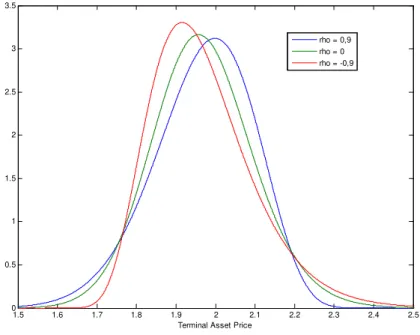
change the form of the RND generating skewness in asset returns. For example, if is
negative, there is a negative correlation between shocks to asset price and volatility, which means that a negative shock to the price will increase the volatility and consequently increase the likelihood of getting further big downward movements. A positive correlation between asset price and volatility has the opposite e¤ect. The …gure 4-1 shows the e¤ect
of changing on the RND.
Heston (1993) shows that under stochastic volatility assumptions, the European call options have the closed form given in equation (3.6).
In order to obtain the true density and its associated summary statistics, we apply
the second partial derivative of equation C(St; vt; X; T) with respect to the strike price
1.5 1.6 1.7 1.8 1.9 2 2.1 2.2 2.3 2.4 2.5 0 0.5 1 1.5 2 2.5 3 3.5
Terminal Asset Price
rho = 0,9 rho = 0 rho = -0,9
Figure 4-1: Implied RND under aternative values for the correlation parameter
In order to test the ability of the estimation methods tested to capture a wide range of possible shapes of the "true" RNDs, we establish a set of six scenarios divided into low and high volatility and which have three levels of skewness (strong negative skewness, weak positive skewness and strong positive skewness) as in Cooper (1999).
Table 4-1: Parameters used in Heston model under each scenario
Strong negative Skew Weak positive skew Strong positive skew
Low volatility
Scenario 1
= 2;p = 0:1
= 0:1; = 0:9
Scenario 2
= 2;p = 0:1
= 0:1; = 0
Scenario 3
= 2;p = 0:1
= 0:1; = 0:9
High volatility
Scenario 4
= 2;p = 0:3
= 0:4; = 0:9
Scenario 5
= 2;p = 0:3
= 0:4; = 0
Scenario 6
= 2;p = 0:3
= 0:4; = 0:9
average of historical strike prices between January 1996 and February 2010 (end of month prices) for each delta, in order to obtain the average interval between strike prices for this period. Because the quotes are given in volatility in terms of delta, at each considered date, we converted the deltas into strike prices using the formulas
Xcall =Ste N
1
( callerusdT) p
T+(rbrl rusd+ 2=2)T (4.2)
Xput =SteN
1
( puterusdT) p
T+(rbrl rusd+ 2=2)T ,
whereStis the USDBRL exchange rate (the price of one unit of the US dollar, which is the
foreign currency, expressed in BRL real, the domestic currency),rbrl is the domestic
risk-free interest rate (Brazilian interest rate) and rusd the foreign interest rate (US interest
rate) Espen (2007). As with strike prices, in the Heston model we also used the average and the volatility of the spot USDBRL FX rate for the period starting on June 2006
and …nishing on February 2010 for S0 (USDBRL price att = 0) and v0 (volatility of the
USDBRL price at t = 0). The interest rates rbrl and rusd are also an average from the
money market rates (US Libor and SICOR for Brazil) for the same period and have a maturity of 1, 3 or 6 months, depending on the maturity of the "true" RND.
In total, we generate six scenarios for each maturity which results in eighteen di¤erent RNDs. The other parameters used for producing the di¤erent scenarios are the same as in Bu and Hadri (2007) and Cooper (1999). The authors chose the long-run volatility based on the levels of implied volatility typically observed within equity markets and for the low volatility scenarios chose the long run volatility typically observed in stock index, currency and interest rate markets.
in the real world.
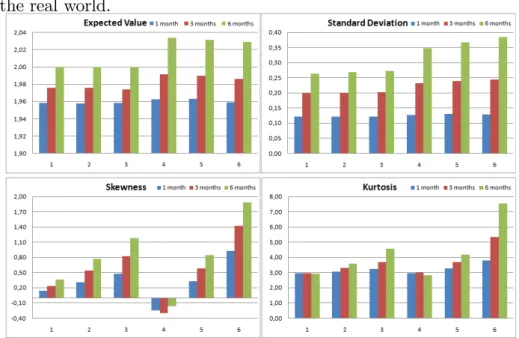
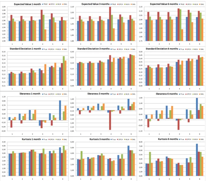
Figure 4-2: Summary statistics of the "true" RND obtained through the Heston model
The summary statistics for the eighteen RNDs obtained through the Heston model are presented in …gure 4-2. The wide range of di¤erent shapes that the di¤erent RNDs can assume can be seen. For example, the skewness range between -0.1651 and 1.8839 and the kurtosis between 2.8316 (thin tails) and 7.5411 (fat tails) in the high volatility scenario for the 6-month horizon. We can also see that the variance increases with the maturity, as it should be expected.
To test the robustness of the MLN, SML and DFCH models in recovering the "true" RNDs, we …rst derive the call option prices using equation (3.6) in section 3.1.2 for each combination of scenario and maturity. We then add a uniformly distributed random noise perturbation in prices of size between minus half and half of the tick size (according to BM&FBOVESPA, the minimum tick size is 0.001) as in Bliss and Panigirtzoglou (2002). Given these shocked option prices, we use the MLN, SML and DFCH methods (the details of the optimization process are described in section 4.4) to estimate the RNDs. This process of …rst shocking prices and then …tting the RND is repeated 500 times for the eighteen combinations of maturities and scenarios (Monte Carlo Simulation).
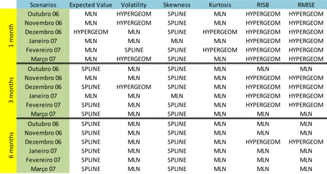
the USDBRL option market, we proceed with the calibration of the Heston model for the end of month USDBRL option quotes between June 2006 and February 2010 (the results are presented in …gure 11-9 in Appendix B) and we also produced the tests described above for 12 dates (6 low volatility dates and 6 high volatility dates). For the low volatility dates we select the period between October 2006 and March 2007 (before the increased problems regarding the subprime crisis). For the high volatility dates we select the period between September 2008 and February 2009 (peak of the subprime crisis). For these periods, we generate the "true" RNDs using the calibration parameters and the strike prices obtained for each tested date.
The di¤erent methods are then compared using some statistical measures that will be described below.
4.3
Statistics used in comparison of di¤erent
tech-niques
In this thesis the di¤erent methods were compared using di¤erent approaches adopted by di¤erent authors.
In Cooper (1999) and Bliss and Panigirtzoglou (2002) the mean, standard devia-tion, skewness and kurtosis of the estimated RNDs were analyzed. However, Bliss and Panigirtzolou focused on stability analysis.
In Cooper the robustness of the MLN and SML methods was studied by comparing the mean of the summary statistics obtained from the Monte Carlo simulations with the
summary statistics of the "true" RNDs. The process of shocking the prices 4 and then
…tting the RNDs was repeated 100 times. The author also tested the stability of these models by analyzing the standard deviation of the summary statistics, arguing that the model with the best performance in terms of stability has a lower standard deviation for
the di¤erent descriptive statistics. He concluded that the SML method performed better than the MLN method in terms of accuracy and stability.
Bliss and Panigirtzolou tested the stability of the MLN and SML methods, but instead of shocking the …tted prices obtained from the Heston model, they introduced a noise in market prices. The authors believed a good estimation method would have better behavior in the convergence results of the processed simulations. These authors did not adopt the methods followed by Cooper, arguing that goodness-of-…t results outside the range of available strike prices (tails of the distribution) can be unreliable, in the sense that there is an in…nite variety of probability masses in the tails of the RNDs obtained. In fact, the summary statistics with higher moments like skewness and kurtosis are very sensitive to the tails of the distribution, and the data outside the set examined is heavily dependent on the estimation method used. For example, when the assumed PFD has a double-lognormal functional form, the MLN estimation method may do better than the other methods. We agree with these arguments and hence we give more importance to the RMISE analysis (root mean integrated analysis) as in Bu and Hadri (2007).
Bu and Hadri (2007) tested the accuracy and stability of the DFCH and SML methods using the root mean integrated squared error (RMISE), which has the advantage of being less sensitive to the tails of the distribution. Another advantage of RMISE is that it can be broken down into RISB (root integrate square bias) that measures the accuracy and RIV (root integrated variance) which indicates the stability of the distribution. As in Cooper (1999), Bu and Hadri also compared the performance of the methods in terms of a "true" PDF produced from an assumed Heston stochastic volatility price and using the pseudo-prices generated from the PDFs as input. For each combination of maturity and scenario, the authors carry out 500 simulations and …nd that in the majority of the cases the DFCH method performs better than the SML method in terms of accuracy (RISB) and stability (RIV).
Lee (2008), and using the mean, standard deviation, skewness and kurtosis summary statistics as in Cooper (1999) and Bliss and Panigirtzoglou (2002).
A de…nition of these statistics is provided below:
i. mean: expected value of the implied PDF.
ii. standard deviation: square root of the variance of the implied PDF.
iii. skewness: the third central moment of the implied pdf standardized by the third
power of the standard deviation.
Skewness= E[X X]
3
3 (4.3)
It provides a measure of asymmetry, measuring the relative probabilities above and be-low the mean. By weighting the relative probabilities through the cubic distances, the weighting of the relative probabilities above the mean becomes positive and the weighting of the relative probabilities below the mean becomes negative.
iv. kurtosis: the fourth central moment of the implied pdf standardized by the fourth
power of the standard deviation. Provides a measure of the degree of "fatness" of the tails of the implied pdf. The kurtosis of the normal distribution is equal to three. A higher kurtosis usually implies a greater probability for extreme changes. This means that a distribution with a higher kurtosis when compared with the normal distribution has fatter tails than the normal distribution (normally associated with a greater degree of "peakedness" in the centre of the PDF).
Kurtosis= E[X X]
4
4 (4.4)
v. RMISE: the root mean integrated squared error. By considering f(S^ t) as the
estimator of the true RND, then the RMISE is de…ned as
RM ISE( ^f) =
s E[
Z 1
1
( ^f(St) f(St))2dSt] (4.5)
the RND. It is a measure of the quality of the estimator and is not as sensitive to the tails of the distribution as the skewness and kurtosis.
The squared of RMISE can also be broken down into the sum of the squared RISB (root integrated squared bias) and squared RIV (root integrated variance):
RM ISE2( ^f) = RISB2( ^f) +RIV2( ^f) (4.6)
RISB( ^f) =
sZ 1
1
(E[ ^f(St)] f(St))2dSt] (4.7)
RIV( ^f) =
sZ 1
1
E[( ^f(St) E[ ^f(St)])2]dSt (4.8)
In the thesis we tested all the statistics explained above. However, because of the limitations of skewness and kurtosis in evaluating PDFs, we give more importance to RMISE as a measure of the overall quality of the estimator, whereby RISB is the measure of the accuracy and RIV is the measure of the stability.
4.4
Numerical aspects of estimating option prices
using MLN, SML and DFCH
The optimizations we have performed for the calculus of the theoretical option prices and estimation of the risk-neutral densities using Double-Lognormal Function (DLN), the Smoothed Implied Volatility Smile (SML) and the Density Functional Based on Con‡uent Hypergeometric Function (DFCH) were produced using the MATLAB software.
4.4.1
Double-Lognormal Function
density (RND) that is consistent with various stochastic processes for the underlying as-set (instead of specifying underlying asas-set price dynamics as in Black and Scholes’ model, which leads to a unique terminal RND). Using the MLN method, the RND is a weighted sum of lognormal density functions because according to Bahra the asset price distrib-utions are closer to the lognormal distribution. For our purposes, we follow Bahra and adopt a Mixture of two lognormals in the estimation of the risk-neutral densities from the pseudo-option prices calculated through the Heston model (as described in section 4.2).
The …ve parameters ( 1; 2; 1; 2; w) are estimated through the minimization problem
de…ned in equation (3.15). The part of the minimization problem that corresponds to the non-arbitrage condition, restricting the expected value of the RND to be equal to the forward price of the underlying asset, is de…ned in our algorithm as the price of the underlying asset minus the theoretical price of a call option (using MLN model) with a strike price of 0, which has the same meaning as equation (3.15) but in a di¤erent form. In fact, this martingale condition means that for a strike price of 0, the option will always be exercised and at maturity it will be worth the value of the underlying asset. Therefore, we must solve the minimization problem:
min
1; 2; 1; 2;w
n
X
i=1
[c(X; ) bc]2+ [S c(0; )] (4.9a)
Due to the symmetry problems discussed in section 3.2.1, we impose 1 > 2 (the …rst
density will have a larger standard deviation than the second one). The optimization was carried out using MATLAB with a non-linear least squares optimization algorithm and we follow the optimization steps proposed in Jondeau et al. (2006). We start by de…ning
a vector of values for the weight parameter w in the interval [0;1]. The points in this
vector are equally spaced at intervals of 0.1. We then proceed to the optimization along
the grid ofwvalues and obtain the values for 1; 2; 1; 2; w that minimize our problem.
4.4.2
Density Functional Based on Con‡uent Hypergeometric
Function
This method, described in section 3.2.1, was developed in Abadir and Rockinger (2003) and consists of the use of a formula that encompasses various densities, like normal, gamma, inverse gamma, weibull, pareto and mixtures of these statistical densities.
As explained in section 3.2.1, the number of parameters to be estimated using this model was reduced to seven, due to the restrictions:
c2 = 1 +a4
p
b4 ; (4.10)
a4 =
1
2p b4
1 a1( b2) a2
(a3)
(a3 a2)
; (4.11)
c1 = c2m2; (4.12)
b1 = 1 +a2b3; (4.13)
a5 =
1
2; (4.14)
a6 =
1
2; (4.15)
E(X) =a1
(a3)
(a3 a2)
( b2) a2(m1 m2) +m2: (4.16)
The minimization de…ned in equation (3.23a) (regardless of the method used, the objective is to minimize some function of the squared distance between the observed option prices and the …tted prices derived from the estimated PDF) was performed in Matlab using non-linear least square optimization.
As described in section 4.2, the estimation of the risk-neutral densities used the pseudo-option prices calculated through the Heston model as input.
These parameters coincide with the parameters of a Gaussian RND for the third term of equation (3.17):
a5 =
1
2; a6 =
1
2; b4 =
1
2 2(K); m2 =mean(K): (4.17)
Moreover, for the second-term of equation (3.17) the starting parameters correspond to the parameters of a restricted gamma RND:
b1 = 1 +a2b3; b3 = 1; a3 =a2+ 2; a2 = 4; m1 =m2 (4.18)
Owing to the highly non-linear nature of the function, it was also important to state lower and upper bounds to the parameters of the function during the optimization processes in order to achieve better stability and …t for the results obtained.
4.4.3
Smoothed Implied Volatility Smile
In the estimation of the RNDs through the SML model we used the method proposed in Bliss and Panigirtzoglou (2002) which consists of an interpolation of volatility/delta space using a natural smoothing cubic spline, whereby the second-order derivatives in
the extreme knot points were 0 (spline function is linear outside the range of available
data). This method is explained in detail in section 3.2.1.
The variable regarding the weight parameterwin equation (3.32) is described by Bliss
and Panigirtzoglou as a source of price error. It is known that in the context of the Black and Scholes formula, the only unobservable parameter is volatility ( ), which means that
the uncertainty regarding the PDF lies in . The greek vega (v) measures the relationship
between volatility and option price (v = dC
d ) and re‡ects the uncertainty concerning
the volatility. The value of v is approximately0for far deep-out-the-money options and
reaches its maximum for at-the-money options5. The authors use thisv weighting when
…tting the volatility smile because this weighting scheme places more weight on near-the-money options and less weight on away-from-the-near-the-money options. However, the authors admitted that it was di¢cult to choose a good weighting scheme that takes into account all the sources of price error. In this thesis we tested the SML model using both vega
weighting (wi =vi) and equal weighting (wi = 1) and observed that the performance is
similar for both (with a slight improvement for the vega weighting).
The smoothed parameter in function (3.32) , , multiplies a measure of curvature in function (3.32) and allows the smoothness of the spline and its shape to be controlled. In this thesis we tested this method using the value that minimizes the RMISE (root mean integrated squared error) as the smoothed parameter. Nevertheless, because in the real world we don’t know the "true" RND, we are unable to get the that minimizes RMISE. As such, we also performed the SML technique using a speci…c value for the smoothing
parameter ( = 0:9).
In conclusion, we tested this method using di¤erent schemes for the weighting
para-meter (wi = vi and wi = 1) and for the smoothness of the spline ( that minimizes the
RMISE and = 0:9). We observed that the performance is very similar for the di¤erent
Chapter 5
Comparison of di¤erent methods
using the Cooper scenarios
The di¤erent methods tested in this thesis, the Double-Lognormal Function (DLN), the Smoothed Implied Volatility Smile (SML) and the Density Functional Based on Con‡uent Hypergeometric Function (DFCH) were compared in terms of accuracy and stability. The performance of the three techniques was measured based on two di¤erent approaches: analysis using the summary statistics (mean, standard deviation, skewness and kurtosis) and analysis using the RMISE (root mean integrated squared error) as explained in section 4.3.
this approach, the model with better accuracy would present mean values of summary statistics closer to the "true" RND and the model with more stability would have a lower standard deviation of summary statistics.
However, as explained in section 4.3, skewness and kurtosis are very sensitive to the tails of the distribution and the data outside the examined set is heavily dependent on the estimation method used. That is why we also follow the approach used in Bu and Hadri (2007), who tested the accuracy and stability of the DFCH and SML methods using the root mean integrated squared error (RMISE), which is a more reliable measure of the robustness of the RND estimators.
5.1
Analysis using mean, standard deviation,
skew-ness and kurtosis
5.1.1
Accuracy
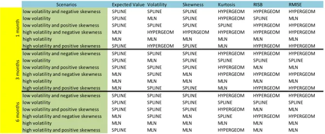
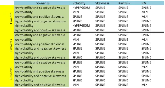
The accuracy using this approach was analyzed by comparing the average values of the mean, standard deviation, skewness and kurtosis estimated from the 500 Monte-Carlo simulations, which were applied to each combination of scenario and maturity (the scenarios are de…ned in table 4-1). The method with the best performance has an average value of the summary statistics that is close to the "true" ones (…gures 5-1 and 5-2).
Scenarios Expected Value Volatility Skewness Kurtosis RISB RMISE
low volatility and negative skewness SPLINE SPLINE SPLINE HYPERGEOM HYPERGEOM HYPERGEOM
low volatility SPLINE MLN SPLINE HYPERGEOM SPLINE MLN
low volatility and positive skewness SPLINE SPLINE SPLINE SPLINE HYPERGEOM HYPERGEOM
high volatility and negative skewness MLN HYPERGEOM HYPERGEOM HYPERGEOM HYPERGEOM HYPERGEOM
high volatility MLN MLN MLN MLN MLN MLN
high volatility and positive skewness SPLINE HYPERGEOM SPLINE MLN HYPERGEOM HYPERGEOM
low volatility and negative skewness SPLINE SPLINE SPLINE HYPERGEOM HYPERGEOM HYPERGEOM
low volatility SPLINE MLN SPLINE SPLINE SPLINE SPLINE
low volatility and positive skewness SPLINE SPLINE SPLINE HYPERGEOM MLN MLN
high volatility and negative skewness MLN SPLINE MLN HYPERGEOM HYPERGEOM HYPERGEOM
high volatility MLN MLN MLN MLN MLN MLN
high volatility and positive skewness MLN SPLINE SPLINE MLN HYPERGEOM HYPERGEOM
low volatility and negative skewness SPLINE SPLINE SPLINE HYPERGEOM HYPERGEOM HYPERGEOM
low volatility SPLINE SPLINE SPLINE SPLINE SPLINE SPLINE
low volatility and positive skewness SPLINE SPLINE SPLINE HYPERGEOM MLN MLN
high volatility and negative skewness MLN SPLINE MLN SPLINE HYPERGEOM HYPERGEOM
high volatility MLN MLN MLN MLN MLN MLN
high volatility and positive skewness SPLINE MLN MLN HYPERGEOM MLN MLN
1
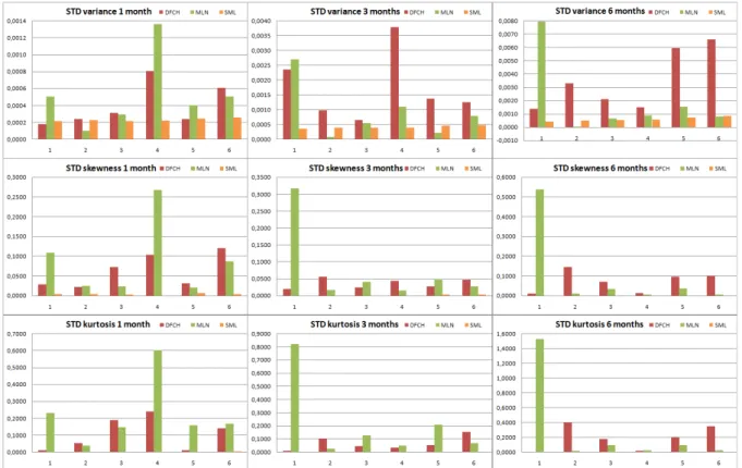
mon
th
3
mont
hs
6
mont
hs
Figure 5-2: Summary statistics obtained for Heston model (true density) and mean of summary statistics obtained for DFCH, MLN and SML methods. The results estimated
for the SML method were processed withv weighting and with the smoothing parameter
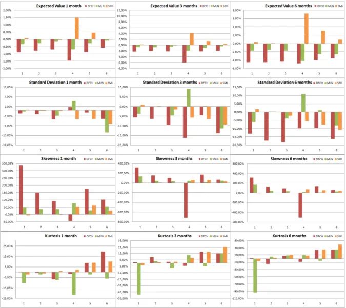
Figure 5-3: Di¤erence between the "true" and the mean summary statistics in per-centange of the "true" statistics.The results estimated for the SML method were
Expected Value
If we look at the expected value, we see that the SML method has a better performance than the MLN method, with the exception of scenarios 4 and 5 (for all the maturities), where the MLN model is slightly closer to the "true" RND. The DFCH method has a biased expected value for almost all scenarios and maturities.
Standard Deviation
Analyzing the volatility, we see that for "one month to maturity" the SML outperforms the DFCH and the MLN methods in scenarios 1, 2 and 3. The DFCH method almost always has the worst performance, with the exception of scenarios 4 and 6, where it has the less biased implied volatility.
In the "three months to maturity" the SML technique has a better …t in scenarios 1, 3, 4 and 6. The DFCH has the least …tted implied volatility.
Considering the six-month term, we notice that the SML and MLN methods outper-form the DFCH one, with the SML method showing better results for the low volatility scenarios and the MLN one the best in the high volatility scenarios.
In general terms, we see that the SML method has a better performance in capturing the volatility of the "true" density. The volatility of all tested RNDs increases in line with longer time to maturity, which con…rms the higher uncertainty attached to longer maturities.
Skewness