A Work Project, presented as part of the requirements for the Award of a Masters Degree in Economics from the Faculdade de Economia da Universidade Nova de Lisboa
DOES CORRUPTION DRIVE THE STOCK MARKET?
ANA RAQUEL DA COSTA PINHEIRO
1(MST14000195)
A Project carried out on the Macroeconomics course, with the supervision of:
Professor José Tavares
January 2010
1 I thank my Work Project advisor for insightful suggestions and support. A special thanks to my parents for revising the text and to Afonso Eça for the patience and guidance.
2 Abstract
We estimate the effect of corruption on the stock markets returns using as controls gross domestic product growth, inflation, unemployment growth, monetary base growth and institutional variables. The results show that in more developed countries corruption is inversely related to the stock market returns. In developing economies, on the other hand, there is empirical evidence supporting the second-best theory: higher levels of corruption impact positively on the stock markets returns. Furthermore, while per capita gross national income cannot account for corruption coefficients on the stock market, inflation seems to be positively related to the latter.
3 1. Introduction
“Corruption is an act in which the power of public office is used for personal gain in a manner that contravenes the rules of the game” [Jain (2001)]. According to the World Bank, “corruption is the single greatest obstacle to economic and social development”. Plus, “Milton Friedman’s basic position is that the only social responsibility of business is to increase profits, as long as the company stays within the rules of law” (Baron, 2007).
Many authors have discriminated diverse kinds of corruption. Shleifer and Vishny (1993) divide corruption into two different regimes: “productive corruption”, when one is sure to get the good or service intended (license, permit, etc.) after paying for the bribe (Russia under Communism); and “wasteful corruption”, in the case where the public official may not hand out anything to the briber, receiving a fee for no service at all (as in many African countries). In this latter case, one is not certain to obtain the good or service even after paying the bribe, and moreover, the official can always ask for more bribes.
As to the specific case of the stock market returns, there are also two distinct economic links which can explain the influence of corruption. On the one hand, the expected effect of corruption in a country’s economic activity should be negative and, thus, stock returns should be lower. In other words, both bribes and the extraction of economic rents represent the deviation of resources from the formal sector (namely from public investment) in the case of corruptive behaviour by public officials. Fewer inputs applied by the government would consequently induce a lower level of investment and lower returns, reflected on the stock market as a proxy for economic growth.
On the other hand, there are two possible causes for a positive relation between increased corruption and the stock returns. One perspective is that investors, who are aware of the level of corruption within a country, have to be compensated for that risk. Higher returns are demanded to compensate for a “story of corruption” in a given country. To put it differently, if
4 corruption is a priced factor, to invest in a country with higher levels of corruption investors require a higher expected return. Additionally, corruption can be regarded as a tax: when investors anticipate they will have to bear extra costs (like bribing), they may require higher returns as a compensation. The second positive, distinct relationship between these two elements would be a second best solution; in countries where bureaucracy is a major setback to economic activities, a certain level of corruption would be favourable to business environment. An example is Russia in its transition to a market economy: when formal institutions are not reliable, economic activities become dependent on trustworthy networks of entrepreneurs: “One shot, anonymous transactions in the larger market are risky. As a consequence, economic transactions become limited to those in which trust is established through repeated interactions within a close network of associates (…)” [Wydick (2007)]. This study is organized as follows: next section compares and contrasts two opposite streams regarding the effects of corruption on economics, discussing some of the research already performed in this area. Section 3 provides information on the data collected. Section 4 uses OLS regressions to address the impact of corruption and analyses the results. Additionally, country statistics are used to understand why there are distinguished effects of corruption in countries with different economic backgrounds. Finally, Section 5 concludes. References and additional appendices can be found on Sections 6 and 7, respectively.
2. Literature Review
Corruption is not only a matter of bribery; corruption distorts incentives and people’s minds. According to Shleifer and Vishny (1993) “in some developing countries, such as Zaire and Kenya, [corruption] probably amounts to a large fraction of the Gross National Product.” But can we quantify the impact of corruption in the functioning of the economic activity in general? Specifically, quantify the impact on a country’s stock market returns? The main goal of this work is to establish a clear connection between these two elements.
5 Stock market returns have long been regarded as a means to measure overall economic activity and performance and, consequently, economists have come up with severall theories to define the forces that determine the return of the stock market [Sharpe (1964), Fama (1981), Fama and French (1992), for instance]. Some studies have been well succeeded, but even those have latter faced other approaches contradicting their findings [Fama and French (2005) and Shanken and Weinstein (2005) are two good examples]. The purpose of this work is not to fully define all the motion drivers of the stock market, but to check statistically whether corruption could be one of those elements. The approach followed in this essay is the one that points to observable macroeconomic variables as factors that would drive the stock market [Chen et al. (1986), Flannery et al (2002), among many others, test the impact of macroeconomic variables in explaining stock market price]. The main objective pursued is to examine the weight of corruption as one of these forces behind each country’s stock index returns. Moreover, we address the issue of possible differences across countries, establishing a relation between the results and cultural, socioeconomic characteristics.
What, then, can be said about corruption? For a long time it was not considered a significant economic factor influencing the economy. Indeed, there has been a stream arguing that corrupt behavior itself would not impose social losses. Instead, it would facilitate government’s work of allocating scarce resources [Leff (1964) and Lui (1985)]. However, more recently, economic researchers and academics started to associate corruption to diverse social and economic problems [Gould and Amaro-Reyes (1983), Klitgaard (1991) and Keefer and Knack (1995)], such as lower levels of growth and investment [Mauro (1995)], lower tax revenue [Haque and Sahay (1996) and Tanzi and Davoodi (1997)], attracting fewer foreign direct investors [Wei (1997)], larger informal markets [Johnson et al. (1998)] increased military spending [Gupta et al. (2000)] and even higher infant mortality and student dropout [Gupta et
6 al. (2001)]. Finally, Mauro (2002) points the waste of labour hours spent on unproductive transfers of resources as causes for a low marginal product of capital.
In line with this latter strand of thought, Sanyal and Guvenli (2009) found that, when controlling for the level of per capita income, firms from high-income countries are less likely to give bribes: “Prosperous countries create an environment where firms are able to conduct business ethically.” But what effects should we expect from the fact that low-income countries cannot “conduct business ethically”? Should those be always negative? Could it be empirically proved that corruption is always harmful to economic development and stock market return itself? An interesting exercise would be to predict what the intuitive outcome of this essay would be. According to these recent studies, corruption should impact negatively on the economy. But on the side of the stock returns, things could be far more puzzling. Corruption would have a negative impact on stock markets returns if these were actually explained by corruption – the coefficient of corruption on the stock market returns would be negative. However, if the stock market priced corruption, returns would be higher to compensate for that risk, as referred above, and, hence, they would be positively related.
There have already been some attempts to quantify these issues. For example, Ciocchini et al. (2003) look at the bond spread as a proxy for borrowing cost. They examine the difference between the launch spread of market bonds and the rate of a risk-free bond with the same maturity. The higher spread would be associated with a higher probability of default due to emerging markets’ debt. The coefficient on corruption is always negative and significant, corroborating contemporaneous doctrine. Also at the firm level, Ng (2006) finds that corruption should decrease stock valuation, increase the firm’s borrowing cost and is associated with a worse corporate governance. These latter approaches are somewhat similar to our study, but do not include the country’s individual economic performance. What we do is to study the problem of corruption as a factor influencing stock markets, but this time at a country level.
7 3. Data and Methodology
Our sample is formed by 47 developing and developed countries with various economic backgrounds.2 The period studied is from 1984 to 2008, on an annual basis, when data is available - some sources do not present data for the length of time being studied. One of the possible solutions would be to rely on national central banks data, though we decided not to use national sources and to base our work only in internationally recognized data. Therefore, for some countries the period analysed is smaller than the referred 24 years.
First, we had to address the need of measuring corruption in a given country. For that end, two kinds of indices were used: the Transparency International’s (TI) Corruption Perception Index and the PRS Group’s Corruption Index from the International Country Risk Guide (ICRG) - two of the most popular surveys concerning this subject [Ng (2006)].
About Corruption Perceptions Index, published annually since 1995, Lambsdorff (2007) says “the goal of Corruption Perception Index is to provide data on extensive perceptions of corruption within countries. The Corruption Perception Index is a composite index, making use of surveys of business people and assessments by country analysts. It consists of credible sources using diverse sampling frames and different methodologies. These perceptions enhance our understanding of real levels of corruption from one country to another.” It is rated from 0 to 10 points and the higher the rating, the lower the level of perceived corruption in the public sector is. The Corruption Index, on the other hand, is an integrating part of the International Country Risk Guide. The latter is available since 1984, and divided into three subcategories: Political Risk; Economic Risk and Financial Risk. The Political Risk subcategory is in turn constituted by 12 components, one of them being the Corruption Index. As La Porta et al. (1998b) put it, “the ‘corruption index’ is an assessment of corruption in
2 Argentina, Australia, Austria, Belgium, Brazil, Canada, Chile, China, Czech Republic, Denmark, Finland, France, Germany, Greece, Hong Kong, Hungary, India, Indonesia, Ireland, Israel, Italy, Japan, Jordan, Malaysia, Mexico, Netherlands, New Zealand, Norway, Pakistan, Peru, Philippines, Poland, Portugal, Russia, Singapore, South Africa, Spain, Sri Lanka, Sweden, Switzerland, Taiwan, Thailand, Turkey, United Kingdom, United States.
8 Government by International Country Risk Guide. Low scores of this index indicate that ‘high government officials are likely to demand special payments’ and that ‘illegal payments are generally expected throughout lower levels of government’ in the form of ‘bribes connected with import and export licenses, exchange controls, tax assessment, policy protection or loans.” The index scores 0 to 6 points.
At this point, some adjustments had to be made. As stated just before, corruption indices used in this work are available in different scales, raising an obstacle to possible comparisons. We decided to work with a scale of 0 to 10 points. For that end, all the coefficients on corruption from the International Country Risk Guide Index were multiplied by 10/6, to fit Transparency International’s scale. Moreover, the fact that more points are attributed to countries with lower levels of corruption could be misleading. In this sense, both indices appear multiplied by – 1, so that an increase in the corruption index means the country is more corrupt.
While using the stock market as a proxy for the economy, two types of annual percentage returns are used: real and excess returns. Real returns are adjusted for changes in prices due to inflation (keeping the purchasing power of a given level of capital constant over time), whereas excess returns are obtained by subtracting the interest rate (meaning when these are positive, the return of investment is larger than in a market measure, such as an index fund). On the first econometric specification, we study the impact of corruption alone on the stock markets. Then control variables are included in the OLS regressions: gross domestic product, unemployment, monetary base and inflation (whenever excess returns were the endogenous variable – real returns are already adjusted for inflation). Afterwards, institutional variables were also controlled for: bureaucracy quality, law and order and internal peace.
These steps are performed both using panel data (section 4.1) and then at a national level (4.2, 4.3 and 4.4). Panel data are used to study the impact of corruption across countries and
9 time, allowing the use of more information: more data points imply more degrees of freedom. Then, individual country regressions were run. The terminology used is presented in Table 1.
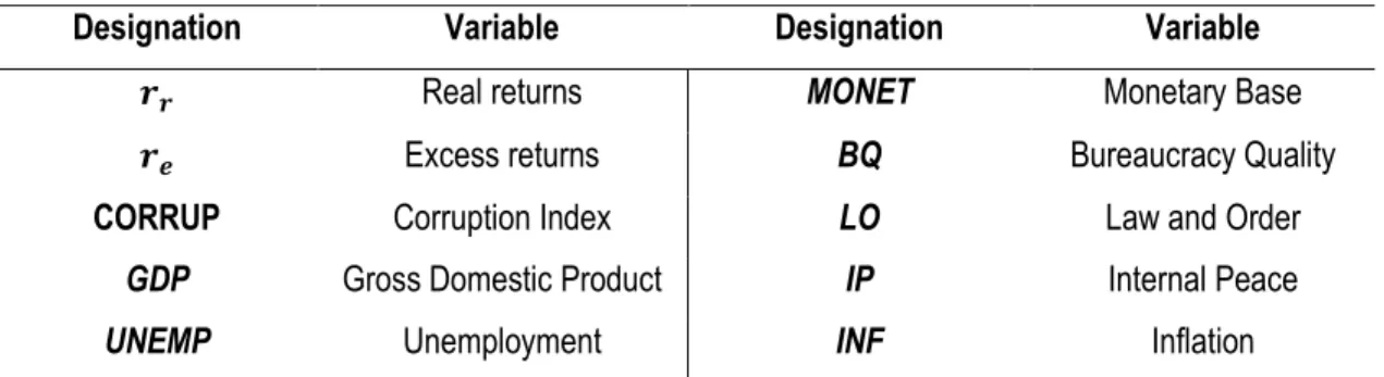
Table 1 – Summary Statistics
Designation Variable Designation Variable
࢘࢘ Real returns MONET Monetary Base
࢘ࢋ Excess returns BQ Bureaucracy Quality
CORRUP Corruption Index LO Law and Order
GDP Gross Domestic Product IP Internal Peace
UNEMP Unemployment INF Inflation
Note: Stock indices were collected from MSCI Barra’s following sections: Developed Markets Standard Core, Emerging Markets Standard Core, Frontier Markets Standard Core and GCC and Arabian Markets Standard Core, USD, price index level, taken annually. Gross domestic product, unemployment, monetary base, interest rate and inflation (computed through consumer price indices) were taken from Bloomberg, OECD, the World Bank, and the International Monetary Fund. Institutional variables are subcomponents of PRS Group’s International Country Risk Guide, Political Risk subcategory. “Internal Conflict” (originally) was changed to “Internal Peace”, so that, in accordance to the other two institutional variables (BQ LO) and to its own rating, larger scores are beneficial and mean less conflicts. For further details on institutional variables’ construction (definition and unit), please check the definition on the appendix, section 7.1.
4. Discussion 4.1 The Big Picture
As stated above, our motivation lies on the fact that the theoretical connection between corruption and stock market returns has not yet been empirically clearly defined. Figures 1 to 4 present a potential relation established by this essay. Distinction is made between real and excess returns and International Country Risk Guide Corruption Index and Transparency International Corruption Perception Index. As in this four figures, for each regression there are four possible specifications, depending on the two types of returns and corruption indices.
For the sake of simplicity, averages of the annual corruption indices were taken for each country, enclosing a period of 24 years for International Country Risk Guide Indices and of 13 years from Corruption Perceptions Indices. Afterwards, the same process was applied to stock
10 returns, being that the length studied is conditional on the availability of corruption indices for each country. The point where the axes cross marks the averages of both series.
Figure 1 - International Country Risk Guide (scaled) and Real Returns
Figure 2 - Transparency International (scaled) and Real Returns
Note: International Organization for Standardization’s country abbreviations available in section 7.2. Brazil and Russia were excluded from the pictures above due to extremely high inflation or interest rate averages.
AR AU AT BE CA CL CN CO CZ DK FI FR DE GR HK HU IN ID IE IL IT JP JO MY MX NL NZNO PK PE PH PT PL SG ZA ES LK SE CH TW TH TR GB US -0,4 -0,3 -0,2 -0,1 0 0,1 0,2 0,3 -10 -9 -8 -7 -6 -5 -4 -3 -2 R e a l R e tu rn s Corruption Indices AR AU AT BE CA CL CN CO CZ DK FI FR DE GR HK HU IN ID IE IL IT JP JO MY MX NL NZ NO PK PE PH PT PL SG ZA ES LK SE CH TW TH TR GB US -0,4 -0,3 -0,2 -0,1 0 0,1 0,2 0,3 -10 -9 -8 -7 -6 -5 -4 -3 -2 R e a l R e tu rn s Corruption Indices
11 Figure 3 - International Country Risk Guide (scaled) and Excess Returns
Figure 4 - Transparency International (scaled) and Excess Returns
Note: International Organization for Standardization’s country abbreviations available in section 7.2. Brazil and Russia were excluded from the pictures above due to extremely high inflation or interest rate averages.
It is enlightening to compare the independent variable from upcoming regressions (the stock returns) to the variable we included as explanatory (the corruption indices). These pictures are quite similar and immediately set the mood for discussion. Why is it that Nordic European countries seem to be the only ones appearing on the 1st quadrant? What do countries in 2nd and 4th quadrant have in common, besides high corruption levels? It may also be interesting to analyse the relation between corruption indices and stock returns, not yet adjusted by inflation or interest rate. Figures 5 and 6 compare corruption indices to “gross” stock market indices.
AR AU AT BE CA CL CN CO CZ DK FI FR DE GR HK HU IN IE IL IT JP JO MY MX NL NZ NO PK PE PH PT PL SG ZA ES LK SE CH TW TH TR GB US -0,2 -0,1 0 0,1 0,2 0,3 0,4 -10 -9 -8 -7 -6 -5 -4 -3 E x ce ss R e tu rn s Corruption Indices AR AU AT BE CA CL CN CO CZ DK FI FR DE GR HK HU IN ID IE IL IT JP JO MY MX NL NZ NO PK PE PH PT PL RU SG ZA ES LK SE CH TW TH TR GB US -0,2 -0,1 0 0,1 0,2 0,3 0,4 -10 -9 -8 -7 -6 -5 -4 -3 -2 E x ce ss R e tu rn s Corruption Indices
12 Figure 5 – MSCI Barra Stock Indices and International Country Risk Guide Indices
Figure 6 – MSCI Barra Stock Indices and Transparency International Indices
Note: International Organization for Standardization’s country abbreviations available in section 7.2.
It can be taken from here that countries presenting stock returns above the average (15%) are generally those which are also addressed higher levels of corruption (as is the flagrant cases of Poland, Russia, Turkey, Argentina, Egypt, Brazil, Mexico and Indonesia, all situated on the 2st quadrant). On the other hand, most of the countries which growth is usually reported as sustained and stable are on the 4th quadrant, implying a level of corruption bellow the average
AR AU AT BE BR CA CL CN CO CZ DK EG FI FR DE GR HK HU IN ID IE IL IT JP JO MY MX MA NL NZ NO PK PE PH PT PL RU SGZA ES LK SE CH TW TH TR GB US 0 0,1 0,2 0,3 0,4 0,5 -10 -9 -8 -7 -6 -5 -4 -3 -2 M S C I B a rr a I n d ic e s Corruption Indices AR AU AT BE BR CA CL CN CO CZ DK EG FI FR DE GR HK HU IN ID IE IL IT JP JO MY MX MA NL NZ NO PK PE PH PT PL RU SG ZA ES LK SE CH TW TH TR GB US 0 0,05 0,1 0,15 0,2 0,25 0,3 0,35 0,4 0,45 0,5 0,55 -10 -9 -8 -7 -6 -5 -4 -3 -2 M S C I B a rr a I n d ic e s Corruption Indices
13 (for instance, most of the European countries). It is also interesting to note the 1st quadrant seams rather “empty”; there are quite few countries gathering both high stock market returns and levels of corruption below the average. Which relation (positive or negative) prevails overall? That is to be analysed in the next subsection.
4.1.1 The Global Effect of Corruption
Firstly, we ran panel data regressions. This means we cannot obtain the weight of corruption at a national level (which is executed later on), but we observe corruption’s effect on stock market across time and countries. We began with the impact of corruption on the stock market alone and afterwards controls were included.3 Notwithstanding, results are quite intricate: we cannot disentangle what sign should corruption coefficient on the stock market have. That is why we decided to analyse the impact of corruption on the stock market at a country level.
4.2 Is Stock Market Driven by Corruption?4
After the panel data approach, in sections 4.2, 4.3 and 4.4 regressions are performed on a national basis. This is the means to accrue country-level coefficients on corruption influence on the stock returns. The first step while analyzing 47 national stock markets was to introduce corruption as the only explanatory variable in individual country regressions:
ݎ௧ = ܿ௧+ ߚଵܥܱܴܴܷܲ௧ + ݑ௧ (1) where ݎ stands either for real or expected returns; ݅ corresponds to the country and ݐ to the year analysed.
At first glance, one may wonder whether this would produce any significant outcome. However, it is remarkable that, of the 47 countries analysed, 24 of them present a significant coefficient on corruption as the only explanatory variable behind stock market returns movement.
3 See section 7.2 in the appendix for detailed results. 4 Table 2 presents the results for this section.
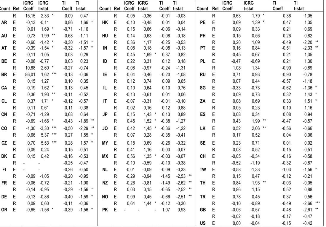
Table 2 – Section 4.2 results Count Ret ICRG Coeff ICRG t-stat TI Coeff TI
t-stat Count Ret ICRG Coeff ICRG t-stat TI Coeff TI
t-stat Count Ret ICRG Coeff ICRG t-stat TI Coeff TI t-stat AR R 15,15 2,33 * 0,09 0,47 HK R -0,05 -0,36 -0,01 -0,03 PE R 0,63 1,79 * 0,36 1,05 E -0,13 -0,11 0,86 1,66 * E -0,10 -0,48 0,01 0,04 E 0,69 1,39 * 0,47 1,35 AU R 0,61 1,69 * -0,71 -1,16 HU R 0,15 0,66 -0,06 -0,14 PH R 0,09 0,33 0,21 0,69 E 0,73 1,99 ** -0,68 -1,11 E 0,14 0,63 -0,08 -0,18 E 0,15 0,56 0,26 0,82 AT R -0,60 -1,42 * -0,30 -1,51 * IN R 0,36 1,17 -0,25 -0,53 PT R 0,20 1,09 -0,49 -2,20 ** E -0,39 -1,54 * -0,32 -1,57 * E 0,08 0,18 -0,08 -0,13 E 0,16 0,84 -0,51 -2,33 ** BE R -0,11 -1,05 0,03 0,29 ID R 0,45 1,69 * 0,37 0,82 PL R -0,45 -0,67 0,21 1,35 E -0,08 -0,77 0,03 0,23 E 0,22 0,31 0,12 0,18 E -0,47 -0,69 0,21 1,30 BR R 10,88 2,60 * -0,27 -0,74 IE R -0,08 -0,97 -0,24 -1,31 RU R 1,08 1,34 -0,90 -0,89 E 86,01 1,62 *** -0,13 -0,36 E -0,04 -0,46 -0,20 -1,08 E 0,71 0,93 -0,90 -0,78 CA R 0,15 1,27 0,10 0,35 IL R 0,12 0,74 0,09 0,65 SG R 0,07 0,44 -0,57 -1,18 E 0,19 1,62 * 0,13 0,45 E 0,10 0,64 0,10 0,76 E -0,33 -0,73 -0,62 -1,36 * CL R 0,36 1,93 ** -0,11 -0,52 IT R -0,13 -0,61 0,01 0,06 ZA R 0,09 0,73 0,32 1,43 * E 0,37 1,71 * -0,12 -0,57 E -0,07 -0,31 -0,01 -0,10 E 0,08 0,69 0,33 1,51 * CN R 0,11 0,61 -0,11 -0,38 JP R -0,02 -0,16 0,12 0,88 ES R 0,05 0,23 0,10 1,16 E -0,71 -1,29 0,68 0,64 E 0,15 1,43 * 0,13 0,89 E 0,08 0,34 0,08 0,94 CO R -0,69 -1,66 * -0,43 -1,89 ** JO R 0,45 1,52 * -0,38 -1,27 LK R 0,43 1,99 ** -0,47 -0,57 E -1,30 -3,30 *** -0,50 -2,29 ** E 0,42 1,45 * -0,36 -1,22 E 0,52 2,06 ** -0,56 -0,66 CZ R 0,66 5,37 *** 0,27 1,55 * MY R 0,07 0,28 -0,35 -0,41 SE R 0,17 0,52 0,04 0,06 E 0,70 5,53 *** 0,28 1,57 * E 0,18 0,69 -0,26 -0,32 E 0,23 0,71 0,01 0,02 DK R 0,09 0,24 -0,15 -0,51 MX R 0,41 1,16 -0,03 -0,07 CH R -0,08 -0,52 -0,15 -0,51 E 0,15 0,42 -0,16 -0,53 E 0,56 1,35 * -0,03 -0,07 E -0,05 -0,34 -0,16 -0,58 FI R - - -0,25 -0,47 NL R -0,10 -0,59 -0,10 -0,38 TW R -0,52 -1,19 -0,32 -0,87 E - - -0,26 -0,50 E -0,01 -0,09 -0,09 -0,33 E -0,58 -1,33 -1,03 -1,56 * FR R -0,09 -1,05 -0,20 -0,95 NZ R -0,29 -0,94 -1,45 -2,53 ** TH R 0,15 0,47 -0,12 -0,21 E -0,06 -0,72 -0,21 -1,00 E -0,26 -0,81 -1,49 -2,62 ** E 0,84 1,93 ** -0,03 -0,05 DE R -0,14 -0,95 -0,39 -1,56 * NO R 0,03 0,15 -0,65 -2,52 ** TR R 0,86 1,15 0,52 0,88 E -0,13 -0,86 -0,40 -1,59 * E 0,09 0,45 -0,66 -2,51 ** E 0,78 0,45 0,37 0,56 GR R 0,09 0,60 -0,11 -0,36 PK R 0,64 1,44 * -0,12 -0,30 GB R -0,10 -0,89 -0,49 -2,66 *** E -0,65 -1,56 * -0,39 -1,56 * E - - - 1,07 0,93 E -0,06 -0,57 -0,48 -2,61 ** US R -0,02 -0,18 -0,17 -0,47 E 0,00 -0,04 -0,15 -0,42
Note: “ - “ stands for insufficient or non-applicable data (for instance, the case of constant series). “R” represents “Real Returns” and “E” “Excess Returns”; “Coeff” stands for “Coefficient”; “Count” for “Country” and “Ret” for “Returns”. Robust t-statistics in parenthesis (* denotes significance for ∝ = 1%; ** for ∝ = 5% ; *** for ∝ = 10%, respectively). Only Corruption coefficients are reported, for the sake of parsimony.
Results are somewhat intriguing. In some countries, the sign of the coefficient is what we expected: less corruption leads to higher stock market returns. Thus, the coefficient is significant and negative. A good example is Norway: when the level of corruption increases 1 unit, there should be a 0,65 p.p. decrease in the real returns, while excess returns decreased by 0,66 p.p. (coefficients significant with ∝ = 2,5%). According to Shleifer and Vishny (1993) definitions, referred in section 2, this would be considered “wasteful corruption”. Contrasting with Norway, there are countries where the coefficient obtained is positive, which means the more corrupt the country is, the better the stock markets performs. For instance, whenever the South Africa is 1 unit more corrupt (according to the international entities), there will be an increase of 0,33 and 0,32 p.p. for excess and real returns, respectively (both significant for ∝ = 10%). In the sense that corruption actually produces a positive impact on the stock returns, it would be regarded as “productive corruption”. What could be the motive behind such different impacts of corruption? We will come back to this issue on section 4.5.
4.3 Corruption and the Economic Basics5
In this subsection control variables were included in the simple regression performed in section 4.2. Basic economic variables were added: Gross Domestic Product Growth (ܩܦܲ ); Unemployment Growth (ܷܰܧܯܲ ) and Monetary Base Growth ( ܯܱܰܧܶ ), obtaining:
ݎ ௧ = ܿ௧+ ߚଵܥܱܴܴܷܲ௧+ ߚଶܩܦܲ + ߚప௧ ଷܷܰܧܯܲ ప௧+ ߚସܯܱܰܧܶ ప௧+ ݑ௧ (2) for real returns. Inflation was also taken into account when explaining excess returns (as explained in section 3, real returns already take inflation into account), but monetary base was excluded from the specification:
16 ݎ ௧ = ܿ௧+ ߚଵܥܱܴܴܷܲ௧+ ߚଶܩܦܲ + ߚప௧ ଷܷܰܧܯܲ ప௧+ ߚସܫܰܨ௧+ ݑ ௧ (3)
Where again ݅ corresponds to the country and ݐ to the year analysed. Of the 47 analysed countries, 29 present significant coefficients on corruption when using economic basic variables as controls. That is, the percentage of significant coefficient of corruption in our sample is now more than 60%. This means there are more countries where corruption has a significant impact than countries where these surveys do not produce any effect on the stock market. Some countries did not possess a significant coefficient on corruption in section 4.2, but with basic economic variables controlled for, they now do. Thus, placing corruption as the only explanatory variable behind the stock market returns may bear an omitted variable problem: we are requiring corruption to “explain too much”, and the coefficient ends up not being significant. Including control variables reveals to be a simple but effective step. Additionally, a remarkable fact which also corroborates the consistency of the results is that almost all the significant coefficients ߚଵ obtained in this section keep their sign relatively to the regression (1).
4.4 Adding the Institutional Element6
According to Mauro (2002), “economists and policymakers have long-recognized that institutions matter in determining economic performance.” In this sense, we used three institutional variables from the International Country Risk Guide: Bureaucracy Quality (BQ), Law and Order (LO) and Internal Peace (IP).7 The specification used for real returns was
ݎ ௧ = ܿ௧ + ߚଵܥܱܴܴܷܲ௧+ ߚଶ ܩܦܲ + ߚప௧ ଷܷܰܧܯܲ ప௧+ ߚସܯܱܰܧܶ ప௧+ ߚହܤܳ௧+ ߚ ܮܱ௧ + ߚܫܲ௧+ ݑ௧ (4) As above, for the excess returns inflation was added to the variables to be controlled for.
6 Results exhibited in Table 4.
7 For instance, Bordo and Rousseau (2006) relate frequent revolutions or coups to lower development at various levels of economic society. See sections 3 and 7.1 for clarifications on institutional variables. A table of correlations is exhibited in the appendix; they are quite high, but corruption coefficient still “survives” them.
Table 3 – Section 4.3 results Count Ret ICRG Coeff ICRG t-stat TI Coeff TI
t-stat Count Ret ICRG Coeff ICRG t-stat TI Coeff TI
t-stat Count Ret ICRG Coeff ICRG t-stat TI Coeff TI t-stat AR R 9,20 2,48 ** 0,19 0,69 HK R -0,05 -0,18 0,09 0,38 PE R 0,53 1,28 0,31 0,47 E 0,95 1,78 * 1,20 2,08 ** E 0,52 1,79 ** 2,16 2,41 ** E 0,42 0,43 0,45 0,59 AU R 0,51 1,01 -0,19 -0,45 HU R 0,39 0,56 -0,26 -0,28 PH R 0,12 0,44 0,10 0,31 E 0,54 1,06 0,21 0,40 E 0,44 0,65 -0,36 -0,46 E 0,35 0,77 0,09 0,24 AT R -0,40 -1,87 * -0,04 -0,26 IN R 0,28 0,84 -0,67 -0,94 PT R 1,56 0,75 0,51 1,32 E -0,65 -1,89 * -0,41 -2,94 *** E -0,16 -0,29 -1,47 -0,96 E 1,29 0,89 0,61 2,67 *** BE R -0,31 -1,51 * 0,09 0,58 ID R -0,70 -1,16 0,22 0,39 PL R 0,22 0,86 -0,55 -2,41 *** E -0,21 -1,44 * -0,16 -1,02 E -0,32 -0,49 0,08 0,06 E -0,01 -0,02 -0,57 -1,99 ** BR R 1,42 1,33 0,32 0,66 IE R -0,35 -3,18 *** -0,56 -2,06 ** RU R -0,52 -0,32 -0,74 -0,61 E -3,88 -1,77 ** 0,40 0,66 E 0,02 0,21 0,00 -0,01 E -0,51 -0,32 -0,66 -0,64 CA R 0,07 0,49 0,49 0,83 IL R 0,02 0,07 0,07 0,21 SG R 0,00 0,02 -0,64 -1,25 E 0,19 1,50 * 0,48 1,10 E -0,25 -0,70 0,07 0,21 E -0,51 -1,31 -0,97 -3,31 *** CL R 0,43 1,86 ** -0,04 -0,16 IT R -0,14 -0,33 0,06 0,24 ZA R 0,34 0,94 0,29 0,66 E 0,42 1,62 * 0,20 0,87 E 0,10 0,31 0,23 1,05 E 0,20 0,88 0,17 0,51 CN R 0,50 1,73 * -0,26 -1,00 JP R 0,12 0,68 0,28 1,21 ES R 0,05 0,19 0,58 2,81 *** E - - 0,50 0,36 E 0,09 0,54 0,31 1,33 E 0,07 0,26 0,13 1,20 CO R -0,36 -0,73 -0,21 -0,68 JO R -0,24 -0,46 -0,57 -1,58 * LK R 0,53 1,82 ** 9,07 2,84 ** E -0,92 -1,37 * -0,12 -0,37 E -0,30 -0,43 -0,51 -1,19 E 0,57 1,46 * -1,47 -0,52 CZ R 0,74 2,55 ** 0,50 1,56 * MY R 0,59 0,63 -0,21 -0,22 SE R 0,08 0,16 -0,37 -0,40 E 0,83 2,83 *** 0,31 1,08 E 0,24 0,77 -0,32 -0,35 E 0,10 0,24 0,16 0,21 DK R -0,62 -1,11 0,23 1,15 MX R 0,40 1,00 -0,69 -0,64 CH R -0,70 -1,41 * 0,01 0,02 E 0,23 0,44 0,21 0,99 E 0,73 1,57 * 0,71 0,43 E 0,03 0,13 0,07 0,21 FI R - - 0,04 0,07 NL R -3,54 -1,92 * -0,45 -0,46 TW R -0,67 -0,73 -0,47 -1,35 E - - -0,35 -0,63 E 0,02 0,09 -0,08 -0,32 E -1,88 -1,22 -1,33 -1,84 ** FR R -0,59 -2,89 ** -0,16 -0,82 NZ R -0,42 -0,90 -0,87 -1,71 ** TH R 0,38 1,13 0,01 0,02 E -0,08 -0,66 -0,29 -1,58 * E -0,24 -0,54 -0,98 -1,69 * E 0,73 1,44 * 0,52 0,59 DE R -0,39 -2,16 *** -0,22 -0,71 NO R -0,33 -1,02 -0,53 -2,03 ** TR R 0,70 0,85 0,51 0,40 E -0,40 -1,99 ** -0,46 -2,00 ** E 0,11 0,36 -0,66 -2,02 ** E 8,02 3,47 *** 0,53 0,31 GR R 0,09 0,34 -0,03 -0,11 PK R 0,99 1,67 * -0,15 -0,34 GB R 0,60 1,49 * -0,17 -0,49 E 0,00 0,00 -0,14 -0,50 E - - - - E 0,78 2,30 ** -0,51 -1,81 ** US R -0,01 -0,10 0,23 0,52 E 0,00 0,03 0,17 0,96
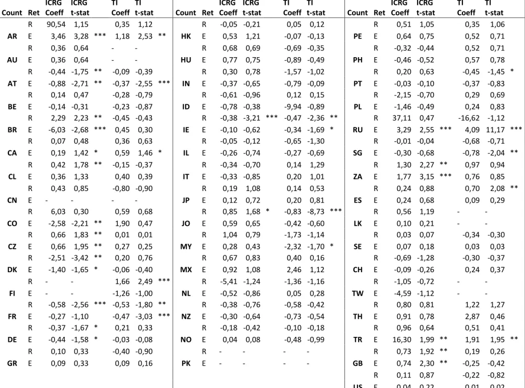
Table 4 – Section 4.4 results Count Ret ICRG Coeff ICRG t-stat TI Coeff TI
t-stat Count Ret ICRG Coeff ICRG t-stat TI Coeff TI
t-stat Count Ret ICRG Coeff ICRG t-stat TI Coeff TI t-stat AR R 90,54 1,15 0,35 1,12 HK R -0,05 -0,21 0,05 0,12 PE R 0,51 1,05 0,35 1,06 E 3,46 3,28 *** 1,18 2,53 ** E 0,53 1,21 -0,07 -0,13 E 0,64 0,75 0,52 0,71 AU R 0,36 0,64 - - HU R 0,68 0,69 -0,69 -0,35 PH R -0,32 -0,44 0,52 0,71 E 0,36 0,64 - - E 0,77 0,75 -0,89 -0,49 E -0,46 -0,52 0,57 0,78 AT R -0,44 -1,75 ** -0,09 -0,39 IN R 0,30 0,78 -1,57 -1,02 PT R 0,20 0,63 -0,45 -1,45 * E -0,88 -2,71 ** -0,37 -2,55 *** E -0,37 -0,65 -0,79 -0,09 E -0,03 -0,10 -0,37 -0,83 BE R 0,14 0,47 -0,28 -0,79 ID R -0,61 -0,96 0,12 0,15 PL R -2,15 -0,70 0,29 0,69 E -0,14 -0,31 -0,23 -0,87 E -0,78 -0,38 -9,94 -0,89 E -1,46 -0,49 0,24 0,83 BR R 2,29 2,23 ** -0,45 -0,43 IE R -0,38 -3,21 *** -0,47 -2,36 ** RU R 37,11 0,47 -16,62 -1,12 E -6,03 -2,68 *** 0,45 0,30 E -0,10 -0,62 -0,34 -1,69 * E 3,29 2,55 *** 4,09 11,17 *** CA R 0,07 0,48 0,36 0,63 IL R -0,05 -0,12 -0,65 -1,30 SG R -0,01 -0,04 -0,68 -0,71 E 0,19 1,42 * 0,59 1,46 * E -0,26 -0,74 -0,27 -0,69 E -0,30 -0,68 -0,78 -2,04 ** CL R 0,42 1,78 ** -0,15 -0,37 IT R -0,34 -0,70 0,14 1,29 ZA R 1,30 2,27 ** 0,97 0,94 E 0,36 1,33 0,40 0,39 E -0,33 -0,85 0,20 1,01 E 1,77 3,15 *** 0,76 0,85 CN R 0,43 0,85 -0,80 -0,90 JP R 0,19 1,08 0,14 0,53 ES R 0,24 0,88 0,70 2,08 ** E - - - - E 0,12 0,72 0,20 0,81 E 0,24 0,68 0,09 0,29 CO R 6,03 0,30 0,59 0,68 JO R 0,85 1,68 * -0,83 -8,73 *** LK R 0,56 1,19 - - E -2,58 -2,21 ** 1,90 0,47 E 0,59 0,65 -0,42 -0,60 E 0,10 0,21 - - CZ R 0,66 1,83 ** 0,01 0,01 MY R 1,04 0,79 -1,73 -1,14 SE R 0,03 0,07 -0,34 -0,30 E 0,66 1,95 ** 0,27 0,25 E 0,28 0,43 -2,32 -1,70 * E 0,07 0,18 0,03 0,03 DK R -2,51 -3,42 ** 0,20 0,76 MX R 0,67 0,83 0,40 0,16 CH R -0,69 -1,28 -0,30 -0,37 E -1,40 -1,65 * -0,06 -0,40 E 0,92 1,08 2,46 1,12 E -0,09 -0,26 0,24 0,37 FI R - - 1,66 2,49 *** NL R -5,41 -1,24 -1,36 -1,16 TW R -1,05 -0,72 - - E - - -1,26 -1,00 E -0,52 -0,86 0,05 0,28 E -4,59 -1,12 - - FR R -0,58 -2,56 *** -0,53 -1,80 ** NZ R -0,38 -0,76 -0,58 -0,42 TH R 0,80 0,81 1,22 1,27 E -0,27 -1,10 -0,47 -3,03 *** E -0,30 -0,64 -0,73 -0,54 E 0,91 0,78 2,87 0,46 DE R -0,37 -1,67 * 0,21 0,33 NO R -0,18 -0,42 -0,10 -0,18 TR R 0,96 0,64 0,51 0,41 E -0,44 -1,58 * -0,03 -0,08 E 0,04 0,08 -0,48 -0,99 E 16,30 1,99 ** 1,91 1,95 ** GR R 0,10 0,33 -0,40 -0,90 PK R - - - - GB R 0,73 1,92 ** 0,19 0,26 E 0,09 0,33 0,09 0,16 E - - - - E 0,74 2,30 ** -0,25 -0,42 US R 0,11 0,87 -0,22 -0,82 E 0,04 0,22 0,01 0,02
Note: “ - “ stands for insufficient or non-applicable data (for instance, the case of constant series). “R” represents “Real Returns” and “E” “Excess Returns”; “Coeff” stands for “Coefficient”; “Count” for “Country” and “Ret” for “Returns”. Robust t-statistics in parenthesis (* denotes significance for ∝ = 1%; ** for ∝ = 5% ; *** for ∝ = 10%, respectively). Only Corruption coefficients are reported, for the sake of parsimony.
After completing all three types of regressions, the most noticeable feature of this exercise is that coefficients rarely change their sign. Of the 564 results obtained, only 4 coefficients change their sign at a given time.8 Still, in 2 of these 4 cases the remaining coefficients keep their sign consistently throughout all the regressions.9
4.5 Analyzing the Results: One-Size Fits All? Not really.
According to the results obtained, we can divide our sample into two different groups.10 Firstly, there are the countries presenting a negative coefficient.11 That is, when corruption indices decrease (meaning the country is less corrupt), the stock market index goes up. This is opposite to the second-best hypothesis theory: there are other countries where an increase in the degree of corruption causes the stock market returns to be higher, and the coefficient is then positive.12 Thus, it may be said corruption is “needed” for the country to function.
Overall, we conclude 34 out of the 47 countries studied present significant coefficients on corruption. But how can the differences in the coefficients be explained? How can we distinguish these two groups? What features is a country likely to have so that corruption has a negative impact on the stock market? And in what cases is it beneficial?
At first glance, we could say these results support both theories: the recent strand has legitimate empirical foundations while supporting the fight against corruption as a means of improving economic performance. However, this seems to be somehow opposite to what
8 Brazil, Jordan, Singapore and UK.
9 For Singapore there is only one significant coefficient, whereas for UK evidence is significant though not clear. 10 UK was not included in any of the groups since evidence on corruption coefficient sign is unclear.
11 Austria, Belgium, Colombia, Denmark, France, Germany, Ireland, Malaysia, Netherlands, New Zealand, Norway, Portugal, Singapore, Switzerland and Taiwan.
12 Argentina, Australia, Brazil, Canada, Chile, China, Czech Republic, Finland, Hong Kong, Indonesia, Japan, Jordan, Mexico, Pakistan, Peru, Poland, Russia, South Africa, Spain, Sri Lanka, Thailand and Turkey.
happens in countries in the 2nd corruption as a second-best soluti and consequences of corruption? institutional setups. On average, c
a positive effect on the stock market returns Bureaucracy Quality, and a higher level of Internal
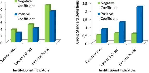
Figures 7 and 8 – Institutio Groups and its Standard Deviations
Source: The PRS Group, International Country Risk Guide.
The standard deviations inside each group are study in section 4.6. That is, t
However, there are also a few countries which seem to be misplaced.
Group’s standard deviation is mainly due to the inclusion of Colombia. On the other hand, Australia, Canada and Finland are clear outliers on the Positive Coefficient Group. If we t those outliers from each bunch
13 This result was achieved through the computation of country
correspondent group. Finally, an average of each of the 2 groups was taken, results which a Figure 7. Same reasoning was applied to standard deviations.
0 2 4 6 8 10 12 G ro u p A v e ra g e s Institutional Indicators Negative Coefficient Positive Coefficient
nd quadrant of figures 5 and 6 above: they proof the
best solution. What then drives these different national approaches and consequences of corruption? A first step towards an explanation may lay on distinct institutional setups. On average, countries that constitute the group where corruption produces ct on the stock market returns are those with lower Law and Order and Bureaucracy Quality, and a higher level of Internal Peace.13
Institutional Contrast between Negative and Positive Coefficient and its Standard Deviations
The PRS Group, International Country Risk Guide.
viations inside each group are also reported since they may motivate our That is, there are, definitely, common elements inside each group. However, there are also a few countries which seem to be misplaced. Negative Coefficient Group’s standard deviation is mainly due to the inclusion of Colombia. On the other hand,
nd Finland are clear outliers on the Positive Coefficient Group. If we t bunch, standard deviations would decrease considerably (0,6
This result was achieved through the computation of country-specific averages, which were then plugged in the correspondent group. Finally, an average of each of the 2 groups was taken, results which a
Figure 7. Same reasoning was applied to standard deviations. Institutional Indicators 0 0,5 1 1,5 2 2,5 G ro u p S ta n d a rd D e v ia ti o n s Institutional Indicators Negative Coefficient Positive Coefficient 20 the existence of What then drives these different national approaches A first step towards an explanation may lay on distinct ountries that constitute the group where corruption produces aw and Order and
between Negative and Positive Coefficient
may motivate our here are, definitely, common elements inside each group. Negative Coefficient Group’s standard deviation is mainly due to the inclusion of Colombia. On the other hand, nd Finland are clear outliers on the Positive Coefficient Group. If we took considerably (0,6 and
specific averages, which were then plugged in the correspondent group. Finally, an average of each of the 2 groups was taken, results which are presented in
0,15 on average, respectively).
which elements actually drive the impact of corruption on each country studied Through gathering World Bank data on these two groups, more distinctions countries displaying a negative relation between higher levels of corruption returns are also those with more
activity of international trade and considerably lower inflation. note that these are also countries far ahe
basic development indicators:
Figure 9 – Development and Macroeconomic Indicators Comparison
Note: All variables’ definitions can be found in the appendix (7.1). 0 10 20 30 40 50 60 70 80 90 100 G ro u p A v e ra g e s
0,15 on average, respectively). By running a panel data regression maybe we can elements actually drive the impact of corruption on each country studied (
athering World Bank data on these two groups, more distinctions could be made: a negative relation between higher levels of corruption and stock markets returns are also those with more solid macroeconomic indicators, heralding a higher level of activity of international trade and considerably lower inflation. Additionally, it is elucidative note that these are also countries far ahead of the Positive Coefficient group when it comes to
Development and Macroeconomic Indicators Comparison
Note: All variables’ definitions can be found in the appendix (7.1). Source: The World Bank.
World Bank Indicators
21 maybe we can identify
(section 4.6). could be made: and stock markets a higher level of onally, it is elucidative to ad of the Positive Coefficient group when it comes to
World Bank Indicators Negative Coefficient Positive Coefficient
22 4.6 Explaining Different Impacts of Corruption
As stated above, the aim of this essay is to quantify the impact of corruptive practices on stock market performance. After having characterized the Positive and Negative Coefficient groups, we regress Doing Business variables on both groups’ corruption coefficients. The panel data sample was formed by countries presenting significant coefficients on corruption and data from Doing Business Indicators (available since 2004).14 Results exhibited on Table 5.
Table 5 – Doing Business Indicators’ and Corruption Coefficient on the Stock Returns
Dependent Variable: Significant Corruption Coefficients
Variables Coefficients
GNI per capita 0,00015 0,000 0,000 0,000 0,000 0,000 0,000
(-2,14)** (-0,449) (0,401) (0,314) (0,115) (0,176) (0,396) Inflation 0,038 0,023 0,023 0,025 0,025 0,023 (5,380)*** (2,763)*** (2,691)*** (2,223)** (2,180)** (2,000)** SB 0,108 0,107 0,107 0,107 0,104 (3,004)*** (2,901)*** (2,874)*** (2,870)*** (2,740)*** DCP -0,012 -0,002 -0,002 -0,001 (-0,138) (-0,224) (-0,283) (-0,166) DE -0,165 -0,162 0,055 (-0,229) (-0,223) (0,069) DI 0,010 0,060 -0,114 (0,017) (0,093) (-0,164) EC 0,001 0,000 (0,332) (-0,016) CB 0,318 (0,664) Adjusted R-square 0,030 0,221 0,273 0,267 0,254 0,248 0,244 Standard Deviation 8,224 7,370 7,121 7,153 7,215 7,244 7,263
Note: Columns represent all 7 executed regressions. Robust t-statistics reported in parenthesis (* denotes significance with ∝ = 1%; ** ∝ = 5% ; *** ∝ = 10%, respectively). Variables’ designation are as follows: SB – Number of Days Needed to Start a Business; DCP - Number of Days Needed to Deal With Construction Permits; DE – Number of Documents Required to Export; DI - Number of Documents Required to Import; EC - Days Required to Enforce Contracts; CB – Years it Takes to Close a Business.
14 Variables from Doing Business database were chosen according to the following method: we took time averages of every variable presented by Doing Business for each country analysed. Afterwards, countries were gathered according to the group they belong: either Positive or Negative Coefficient. Then, group averages were taken for each variable. Those presenting larger differences when the two groups were compared were the ones used in the regression.
15 Per Capita Gross National Income has an extremely small, significant coefficient. This means for every dollar increased in GNI, corruption will actually decrease by -0,0001439 points – an economically relevant result. This regression was also performed with GDP growth instead of GNI per capita, but the first one was not significant.
23 This table clears corruption “interpretation” by national stock markets. That is, these coefficients (which resulted from regressions presented in sections 4.2; 4.3 and 4.4) represent the outcome of corruption on stock returns (though it may be useful to remind these coefficients are estimates, and can only be accountable while bearing that in mind). Corruption can produce a positive impact (being that the country presents a Positive Coefficient) or a negative impact (the Negative Coefficient Group, where when corruption increases, stock returns tend to decrease). What we conclude, maybe surprisingly, is that Gross National Income does not seem to have significant statistical impact on corruption coefficients. Nevertheless, inflation produces an extremely significant positive effect on corruption coefficients. One possible explanation for this is that inflation is a quite “observable” macroeconomic variable, like a benchmark for the state of the whole economy. Therefore, whenever inflation increases and people sense macroeconomic environment is deteriorating, they turn to more corruptive practices. Last, but not least, the number of days needed to start a business is reported as being consistently positively related to corruption coefficients throughout all specifications. Hence, as the predictable time-length needed to accomplish these actions increases, coefficients on corruption will increase, meaning the country is “more corrupt”. This is in accordance with what has been said about corruption enabling businessmen to annihilate red tape obstacles. Actually, the highest R-square was obtained when per capita GNI, Inflation and Days Required for Starting a Business were the sole explanatory variables.
5. Conclusion
First and foremost, the greatest challenge of this study was to include as many countries as possible in our sample, from the most varied economic, cultural and social backgrounds. Our sample is considerably diverse, though it would be interesting to repeat this work in the future, when a larger length of data is available (mainly for developing countries).
24 That being said and despite these obstacles, we found corruption outcomes on the stock market depend on the economic environment inherent to each specific country. Countries empowered with a solid macroeconomic background (reflected on low levels of inflation) and transparent doing business practices have their stock market penalized by corrupt activities. However, in less-developed countries, which do not possess the ease of negotiation of the first ones, stock market returns seem to be favoured by the presence of corruption. This is in accordance with what has been said about corruption enabling businessmen to annihilate red tape obstacles: when bureaucracy is a major setback to economic activities, a certain level of corruption would be favourable to business environment.
As future research, we believe it would be interesting to relate inflation policies to their effectiveness towards controlling corruption levels. Another purposive study would be to include governmental variables in the last regression reported in this essay. Corruption is a wide-spread, deep-seated phenomenon, which can hardly be exhaustively explained. However, knowing the causes of cross-country-differences is one major step towards corruption elimination through adequate and well-fitted policies.
6. References
Bordo, M. D. and Rousseau, P. L. 2006. “Legal-Political Factors and the Historical Evolution of the Finance-Growth Link”, NBER Working Paper, 12035.
Chen, N., Roll, R. and Ross, S. A. 1986. “Economic Forces and the Stock Market”, The Journal of Business, 59 (3): 383-403.
Ciocchini, F., Durbin, E. And Ng, D.T. 2003. “Does corruption increase emerging market bond spreads?”. Journal of Economics and Business, 55: 502-528.
Flannery, M. J. and Protopapadakis, A. A. 2002. “Macroeconomic Factors do Influence Aggregate Stock Returns”, The Review of Financial Studies, 15(3): 751-782.
25 Gould, D.J. and Amaro-Reyes, J. A. 1983. “The effects of corruption on administrative performance”. World Bank Staff Working Papers.
Gupta, S., de Mello, L. and Sharan, R. 2000. “Corruption and military spending”. IMF Working Paper 02/174.
Gupta, S., Davoodi, H. and Tiongson, E. 2001. “Corruption and the provision of health care and education services”, in Jain, A.K., The Political Economy of Corruption, New York: Routledge Press, 111-141.
Haque, N. and Sahay, R. 1996. ‘‘Do government wage cuts close budget deficits? Costs of corruption’’, IMF Staff Papers, 43, International Monetary Fund, 754-78.
Henry, P. B. 2000. “Stock Market Liberalization, Economic Reform and Emerging Market Equity Prices”, The Journal of Finance, 2: 529-564.
Jayasuriya, S. 2005. “Stock Market Liberalization and volatility in the presence of favourable market characteristics and institutions”, Emerging Markets Review, 6: 170-191.
Johnson, S., Kaufmann, D. and Zoido-Lobaton, P. 1998. ‘‘Regulatory discretion and the unofficial economy”. American Economic Review, 88: 387-392.
Kaufmann, D. And Wei, S.J. 1999. “Does ‘grease money’ speed up the wheels of commerce?. Working Paper 7093, NBER.
Klitgaard, R. 1991. Controlling Corruption. University of California Press.
Khan, M. H. 1995. “A Typology of Corrupt Transactions in Developing Countries”. Liberalization and the New Corruption, 27 (2): 12-21.
Lambsdorff, J. G. 2007. The Institutional Economics of Corruption and Reform: Theory, Evidence and Policy. Cambridge University Press.
La Porta, R. Lopez-de-silanes, F., Shleifer, A., Vishny, R.W. 1998. “Law and finance”. Journal of Political Economy, 106:113-155.
26 Leff, N.H. 1964. “Economic development through bureaucratic corruption”, The American Behaviour Scientist, 8: 8-14.
Lui, F. 1965. “An equilibrium queuing model of bribery”. Journal of Political Economy, 93: 760-781.
Mauro, P. 1995. “Corruption and growth”. Quarterly Journal of Economics, 10: 681-712. Mauro, P. 2002. "The Persistence of Corruption and Slow Economic Growth," IMF Working Papers 02/213, International Monetary Fund.
Ng, D. 2006. “The Impact of corruption on financial markets”. Journal of Managerial Finance, 32 (10): 822-836.
Santa-Clara, P., Valkanov, R. 2000. “Political Cycles and the Stock Market”. Anderson School of Management, UCLA, Working Paper.
Shanken, J. and Weinstein, M. I. 2006. “Economic forces and the stock market revisited”, The Journal of Empirical Finance, 13: 129-144.
Shleifer, A. and Vishny, R. W. 1993. “Corruption”, The Quarterly Journal of Economics, 108 (3): 599-617.
Tanzi, V. and Davoodi, H. 1997. ‘‘Corruption, public investment and growth’’, Working Paper 97/139, International Monetary Fund.
Tavares, J. 2001. “Does Foreign Aid Corrupt?”, available at SSRN: http://ssrn.com/abstract=284533 or doi:10.2139/ssrn.284533.
Wei, S.J. 1997. “How taxing is corruption on international investors?”. NBER Working Paper. Wydick, B. 2008. “Property Rights, Governance and Corruption” in Games in Economic Development. 147-169. New York, USA: Cambridge University Press.
27 7. Appendices
7.1 Variables Definition (alphabetic order)
Births attended by skilled health staff. Definition: deliveries attended by personnel trained to give the necessary supervision, care, and advice to women during pregnancy, labor, and the postpartum period; to conduct deliveries on their own; and to care for newborns. Unit: percentage. Source: UNICEF, State of the World's Children, Childinfo, and Demographic and Health Surveys by Macro International.
Bureaucracy Quality. Definition: institutional strength and quality of the bureaucracy. Unit: high points are given to countries where the bureaucracy has the strength and expertise to govern without drastic changes in policy or interruptions in government services; whereas countries lacking the cushioning effect of a strong bureaucracy receive low points because a change in government tends to be traumatic in terms of policy formulation and day-to-day administrative functions. It is scaled from 0 to 6.Source: the PRS Group.
Doing Business Indicators. For a more detailed methodology on the construction of Doing Business variables, visit http://www.doingbusiness.org/MethodologySurveys/.
Exports of goods and services. Definition: value of all goods and other market services provided to the rest of the world. Unit: percentage of GDP. Source: World Bank national accounts data, and OECD National Accounts data files.
GNI per capita. Definition: is the gross national income, converted to U.S. dollars using the World Bank Atlas method (which applies a conversion factor that averages the exchange rate for a given year and the two preceding years, adjusted for differences in rates of inflation
28 between the country), divided by the midyear population. GNI is the sum of value added by all resident producers plus any product taxes (less subsidies) not included in the valuation of output plus net receipts of primary income (compensation of employees and property income) from abroad. Unit: calculated in national currency, is usually converted to U.S. dollars at official exchange rates for comparisons across economies. Source: World Bank national accounts data, and OECD National Accounts data files.
High-technology exports. Definition: products with high R&D intensity, such as in aerospace, computers, pharmaceuticals, scientific instruments, and electrical machinery, sold to the rest of the world. Unit: percentage of manufactured exports. Source: United Nations, Comtrade database.
Imports of goods and services. Definition: value of all goods and other market services received from the rest of the world. Unit: percentage of GDP. Source: World Bank national accounts data, and OECD National Accounts data files.
Inflation. Definition: as measured by the annual growth rate of the GDP implicit deflator shows the rate of price change in the economy as a whole. Unit: the GDP implicit deflator is the ratio of GDP in current local currency to GDP in constant local currency. Source: World Bank national accounts data, and OECD National Accounts data files.
Internal Peace (originally Internal Conflict). Definition: this is an assessment of political violence in the country and its actual or potential impact on governance. Unit: the highest rating is given to those countries where there is no armed or civil opposition to the government and the government does not indulge in arbitrary violence, direct or indirect, against its own people. The lowest rating is given to a country embroiled in an on-going civil war. The risk
29 rating assigned is has a maximum score of 12 points (Very Low Risk) and a minimum score of 0 points (Very High Risk). Source: the PRS Group.
International Country Risk Guide Corruption Index. Definition: “This is an assessment of corruption within the political system. (…) It is more concerned with actual or potential corruption in the form of excessive patronage, nepotism, job reservations, 'favor-for-favors', secret party funding, and suspiciously close ties between politics and business. (…). The greatest risk in such corruption is that at some time it will become so overweening, or some major scandal will be suddenly revealed, as to provoke a popular backlash (…).” Unit: Countries with higher perceived corruption are attributed less points (0 points mean a country has the maximum level perceived of corruption). Those countries presenting lower levels of corruption are awarded with more points, 6 being the maximum number of points. Source: the PRS Group.
Internet users. Definition: people with access to the worldwide network. Unit: percentage of population. Source: International Telecommunication Union, World Telecommunication Development Report and database, and World Bank estimates.
Law and Order. Definition: Law and Order are assessed separately, with each sub-component comprising 0 to 3 points. The Law sub-sub-component is an assessment of the strength and impartiality of the legal system, while the Order sub-component is an assessment of popular observance of the law. Unit: 0 to 6 points, the latter meaning the country is assessed a higher level of law and order. Source: the PRS Group.
Life expectancy at birth. Definition: indicates the number of years a newborn infant would live if prevailing patterns of mortality at the time of its birth were to stay the same throughout its life. Unit: years. Source: World Bank, the United Nations Population Division's World
30 Population Prospects, national statistical offices, household surveys conducted by national agencies, and Macro International.
Mobile cellular telephone subscriptions. Definition: subscriptions to a public mobile telephone service using cellular technology, which provide access to the public switched telephone network, including post-paid and prepaid subscriptions. Unit: percentage of total population. Source: International Telecommunication Union, World Telecommunication Development Report and database, and World Bank estimates.
Mortality rate under-5. Definition: the probability per 1,000 that a newborn baby will die before reaching age five, if subject to current age-specific mortality rates. Unit: probability (0 to 1 range). Source: Harmonized estimates of the World Health Organization, UNICEF, and the World Bank.
MSCI Barra Country Indices. Definition: to construct a country index, every listed security in the market is identified. Securities are free float adjusted, classified in accordance with the Global Industry Classification Standard (GICS®), and screened by size, liquidity and minimum free float. MSCI Barra covers 23 developed, 22 emerging and 29 frontier markets. The MSCI Price Indices measure only the price performance of markets. Dividends are not considered in price indices. Each index measures the sum of the free float-weighted market capitalization price returns of all its constituents on a given day. Unit: USD. Source: MSCI Barra’s website (http://www.mscibarra.com/products/indices/international_equity_indices/definitions.html#Cou ntry).
31 Population growth rate. Definition: annual percentage increase on all residents regardless of legal status or citizenship--except for refugees not permanently settled in the country of asylum, who are generally considered part of the population of the country of origin. Unit: percentage. Source: The World Bank, the United Nations Population Division's World Population Prospects, national statistical offices, household surveys conducted by national agencies, and Macro International.
Poverty rate. Definition: is the annual, national percentage of the population living below the national poverty line. Unit: percentage. Source: Estimates based on the World Bank's country poverty assessments.
Transparency International Corruption Perceptions Index. Definition: measures the perceived level of public-sector corruption based on 13 different expert and business surveys – it is a “survey of surveys”. Unit: A scale of 0 to 10, which attributes the highest number of points to countries with lower level of perceived corruption. Source: Transparency International.
7.2 Appendix Figures
7.2.1 Country Abbreviations by International Organization for Standardization (ISO)
AR Argentina FR France MY Malaysia SG Singapore
AU Australia DE Germany MX Mexico ZA South
Africa
AT Austria GR Greece NL Netherlands ES Spain
BE Belgium HK Hong
Kong
NZ New Zealand
LK Sri Lanka
BR Brazil HU Hungary NO Norway SE Sweden
CA Canada IN India PK Pakistan CH Switzerland
32
CN China IE Ireland PH Philippines TH Thailand
CO Colombia IL Israel PL Poland TR Turkey
CZ Czech
Republic
IT Italy PT Portugal GB United
Kingdom
DK Denmark JP Japan RU Russian
Federation
US United States
FI Finland JO Jordan
7.2.2 Panel Data Results
Index Returns Corruption
Corruption and Base Variables
Corruption, Base and Institutional Variables ICRG Real -0,024 -0,114* 0,163* CPI Real -0,006 -0,013** -0,029** ICRG Excess -0,126 0,085 0,174 CPI Excess 0,001 -0,006 -0,022* 7.2.3 Correlations Bureaucracy Quality Law and Order Internal Peace TI Corruption Perception Index ICRG Corruption Index Bureaucracy Quality 1 0,721 0,532 0,814 0,688
Law and Order 0,721 1 0,694 0,745 0,699
Internal Peace 0,532 0,694 1 0,533 0,527
TI Corruption
Perception Index 0,814 0,745 0,533 1 -