Spectral analysis of embolic signals

(1)

S

p

e

c

t

r

a

l

A

n

a

l

y

s

i

s

o

f

E

m

b

o

l

i

c

S

i

g

n

a

l

s

b byy

A

An

n

a

I

Is

sa

a

be

b

el

l

P

Pe

er

re

ei

ir

ra

a

M

Ma

ar

rt

ti

in

ns

s

L

Le

ei

ir

ri

ia

a

T Thheessiissssuubbmmiitttteeddttootthhee U UnniivveerrssiittyyooffAAllggaarrvvee f foorrtthheeddeeggrreeeeooff D DoouuttoorrnnoorraammooddeeEEnnggeennhhaarriiaaEElleeccttrróónniiccaaeeCCoommppuuttaaççããoo,,eessppeecciiaalliiddaaddeeddee P PrroocceessssaammeennttooddeeSSiinnaall

Área Departamental de Engenharia Electrónica e de Computação Faculdade de Ciências e Tecnologia

Universidade do Algarve January 2005

(2)

RESUMO

Os parâmetros espectrais do sinal Doppler são usados na caracterização de fluxo sanguíneo. No caso particular do fluxo em artéria cerebral média, a caracterização pode incluir a detecção e classificação de embolias.

Para este efeito pretende-se estudar o desempenho de métodos de análise espectral, nomeadamente os que tenham demonstrado bons resultados quando aplicados a sinais Doppler em outras artérias. Para melhor quantificar o desempenho dos estimadores espectrais, é necessário conhecer à priori as características particulares do sinal, facto que se pretende como objectivo final deste estudo.

No sentido de disponibilizar sinais-referência para a análise do desempenho dos

estimadores espectrais na detecção de embolias, foi desenvolvido um simulador de sinais de artéria cerebral média, com e sem embolias. Como entradas do simulador são utilizadas curvas médias extraídas de sinais clínicos, recorrendo a um algoritmo criado para o efeito, o Sequential Phase Shift Averaging. São também definidas pelo utilizador características dos êmbolos, tais como, velocidade, dimensão efectiva e potência devolvidas pela instrumentação ultra-sónica.

Durante este estudo considerou-se o fluxo sanguíneo caracterizado por quatro parâmetros espectrais: frequência máxima, frequência média, raiz quadrada de meia largura de banda, e, variação da potência ultra-sónica ao longo do tempo; este último como sendo o mais relevante para a identificação e diferenciação dos êmbolos.

Recorrendo aos sinais simulados, e, analisando os espectros dos sinais de fluxo sem embolias, verifica-se que a Short Time Fourier Transform estima melhor os parâmetros espectrais referidos do que a distribuição tempo-frequência de

Choi-Williams ou o método paramétrico tempo-frequência de Covariância Modificada. A

análise de espectros de sinais simulados de fluxo com embolias demonstra uma performance idêntica entre os métodos de análise temporal e a Short Time Fourier

Transform, esta na versão em que o espectro do ciclo cardíaco é composto por elevada

taxa de sobreposição de espectros de segmentos desse ciclo. Esta condicionante associada à constatação de que uma mesma embolia é captada distintamente consoante

(3)

o local do ciclo cardíaco em observação induziu a criação de uma nova representação espectral.

A representação proposta, de nome Space-frequency representation, permite a identificação visual da passagem do êmbolo pela janela de observação ultra-sónica. A pesquisa da existência do êmbolo é feita em função da velocidade sanguínea máxima instantânea, e a visualização da potência ultra-sónica por ele retornada é dimensionada adaptativamente de acordo com a relação espaço-frequência instantânea calculada. Esta metodologia permitirá introduzir vantagens significativas no diagnóstico clínico da circulação do fluxo sanguíneo em artéria cerebral média.

(4)

ABSTRACT

Doppler spectrum parameters are used to characterize blood flow. In the particular case of the middle cerebral artery, the characterization may include detection and classification of emboli.

To achieve so, study of the performance of spectral estimator methods, namely those that have produced good results when applied to Doppler signals belonging to other arteries, was deemed. For accurate quantification of the spectral estimators’ performance, a priori knowledge of the signals characteristics is required, which in fact is the final goal of this work.

In order to produce reference-signals to enable analysis of the spectral estimators performance when detecting emboli, a middle cerebral artery signal simulator was developed, with the possibility of including emboli signals. The simulator considered as inputs the mean curves extracted from clinical signals. An algorithm specially developed to do so, the so-called, Sequential Phase Shift Algorithm, computed these mean curves. The simulator user should also specify emboli characteristics such as velocity, effective dimension and power backscattered by the ultrasound instrumentation.

During this study, blood flow was characterized by four spectral parameters: maximum frequency, mean frequency, root mean squared bandwidth, and, ultrasonic power variation over time; the latter being considered as the most relevant for identification and differentiation among emboli.

Making use of the simulated signals, and analysing the spectra of the signals without emboli, we may conclude that the Short Time Fourier Transform estimates the spectral parameters required for embolic analysis with more accuracy than the time-frequency distribution of Choi-Williams or the parametric time-time-frequency Modified Covariance method. Analysis of the spectra obtained from the simulated signals with emboli demonstrates that the time analysis methods perform similarly to the Short Time Fourier Transform, when the latter is used to compute the spectrum of the whole cardiac cycle by computation of highly superimposed spectra of segments of that cardiac cycle. This constraint, in association with the fact that the same embolus is backscattered

(5)

differently according to the place within the cardiac cycle under observation, lead to the development of a new spectral representation.

The proposed representation, named Space-frequency representation, enables the visual identification of the travelling embolus on the ultrasound window of observation. The search for the existence of an embolus is computed based on the instantaneous maximum blood flow velocity, and the visual representation of the backscattered power is adaptively dimensioned according to the instantaneous space-frequency relationship computed. This methodology enables significant improvement on the clinical diagnosis about blood flow in middle cerebral artery.

(6)

Ás minhas queridas avós Natália, Tidi e Teresa

(7)

Mas quando alguém se lembrou Querer mostrar-me, não me opus: É fraca a luz que vos dou,

Mas afinal sempre é luz.

in Este Livro que Vos Deixo…, Volume I, de António Aleixo

(8)

ACKNOWLEDGMENTS

I would like to acknowledge

Universidade do Algarve, for the timely opportunity to conduct this work and for the leave of absence that made it possible;

PRODEP III (Programa de Desenvolvimento Educativo para Portugal), Medida 5, Acção 5.3;

CRUP/Treaty of Windsor for the financial support to the visits made, under the Acções Integradas Luso-Britânicas, to the Medical Physics Department of the Leicester University, UK;

the Medical Physics Department of the Leicester University, for the support of the work conducted there during my visits;

CYTED (Programa de Cooperación Científica y Tecnológica) for sponsoring RITUL (Rede Ibero-Americana de Tecnologias de Ultrasom) and the collaboration with several research groups with common goals;

UNESCO, for the financial support to MAGIAS (Métodos Avanzados de Generación de Imágenes Acústicas).

I would like to express my most sincere thanks

to Prof. Doutora Maria da Graça Ruano and Professor David H. Evans for their supervision, critical suggestions, advices, motivation and patience throughout the course of this work;

to Engª Margarida Madeira e Moura for her friendship, interest and support in all the phases of this work. Without her help it would have been very difficult to overcome some of the problems in the course of this work;

to Professor Wagner Coelho de Albuquerque and to Professor Eduardo Moreno for their most valuable advices and encouragement when I most needed it;

to my mother and my brothers José and Manuel for their constant support and love, and to my dearest nephews Manuel and Rita for their comprehension and patience;

(9)

FIGURES

Figure 1.1 – Practical work addressed in each chapter of the thesis...5

Figure 2.1 – Piezoelectric effect and inverse piezoelectric effect...8

Figure 2.2 – Scatter concept ...9

Figure 2.3 – Reflection and refraction of the sound waves on plane surfaces...9

Figure 2.4 – Principle of operation of Doppler ultrasound in diagnosis...11

Figure 2.5 – Doppler angle...12

Figure 2.6 – Simplified scheme of Pulsed Wave Doppler equipment. ...14

Figure 2.7 – Excerpt of an MCA TCD signal...14

Figure 2.8 – Temporal bone structure ...15

Figure 2.9 – Simplified scheme of the cardiovascular system...16

Figure 2.10 – Heart...17

Figure 2.11 – Blood pressure varying as a function of time...18

Figure 2.12 – Distribution of the extra and intracranial arteries...20

Figure 2.13 – Blood composition ...21

Figure 2.14 – Doppler frequency spectrum ...26

Figure 2.15 – Time-frequency representation of Doppler spectrum...27

Figure 2.16 – Time frequency representation of an MCA TCD signal. ...27

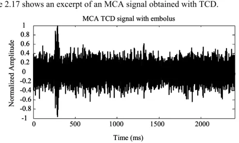
Figure 2.17 – Excerpt of an MCA TCD signal with an embolus. ...33

Figure 2.18 – Time frequency representation of an MCA TCD signal ...33

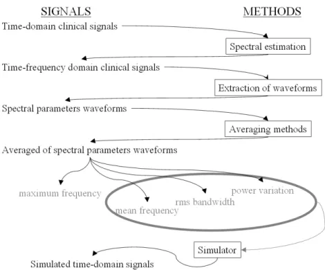
Figure 3.1 – Methods and signals used in this chapter. ...39

Figure 3.2 – Modified Geometric Method for time n. ...45

Figure 3.3 – ECG over a cardiac cycle...47

Figure 3.4 – PFS algorithm schematic representation ...47

Figure 3.5 – MCA maximum frequency waveform extracted from clinical data...52

Figure 3.6 – Averaging methods and methods for delimitating the signals studied in this work. ...55

Figure 3.7 – Time-frequency representation of a denoised MCA Doppler blood flow signal. The significant part of the spectrum is shown in detail. ...57

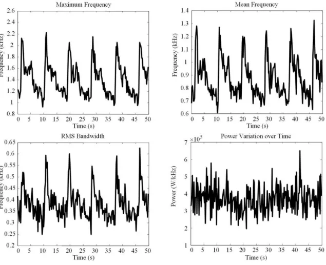
Figure 3.8 – Spectral parameters waveforms taken out of a MCA Doppler signal ...58

Figure 3.9 – Typical appearance of the clinical ECG signals...59

Figure 3.10 – ECG division by R wave: a) Maximum of each segment of length N1; b) After removal of extra flags (using M1); c) Final removal of the remaining extra flags (using rf); d) Minima before maxima (using M2); e) Zero-crossing; f) R wave flagged in the ECG signal ...61 Figure 3.11 – Cycles identification by PFS. a) Original maximum frequency waveform; b) Maximum of each segment, after the moving average, defined by N1; c) After removal of extra flags (using M1); d) Final removal of the remaining extra flags (using rf); e) Maxima of the first gradient (using M2); e)

(14)

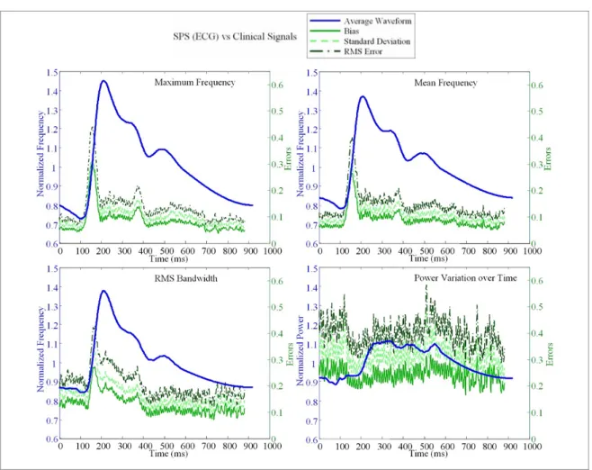
Maximum rate of change of the gradient (using M3); f) Pulse-foot flagged on the moving average of the maximum frequency waveform...62 Figure 3.12 – Rough identification of the cardiac cycles. a) the process of delimitation of the cycles; b) the portion of the file that will be in the current segment appears distinguished; c) all the cycles within the file delimited by the windows. ...64 Figure 3.13 – Schematic representation of the WFA algorithm ...65 Figure 3.14 – Maximum frequency waveform with feature points ...66 Figure 3.15 – Average signals representing the maximum frequency, mean frequency, rms bandwidth and power variation, generated with the WFA. Clinical waveforms, feature points, and additional points are also represented. ...67 Figure 3.16 – Average signals representing the maximum frequency, mean frequency, rms bandwidth and power variation, generated with the SPS and the ECG. Clinical waveforms, feature points, and additional points are also represented...69 Figure 3.17 – Average signals representing the maximum frequency, mean frequency, rms bandwidth and power variation, generated with the SPS and the PFS. Clinical waveforms, feature points, and additional points are also represented...70 Figure 3.18 – Average signals representing the maximum frequency, mean frequency, rms bandwidth and power variation, generated with the SPS having the signals been roughly cut. Clinical waveforms, feature points, and additional points are also represented. ...71 Figure 3.19 – Adapted WFA method: average waveforms errors versus clinical waveforms. Note that the left hand scale refers to the average waveforms and the right hand scale to the errors. ...73 Figure 3.20 – Adapted WFA: some feature points from clinical waveforms versus the average waveforms. The feature points considered are minimum systolic (D), peak systole (S), diastolic notch (N), and mean value (M). ...75 Figure 3.21 – SPS: amount of shift suffered by the cycles (each bin corresponds to 20ms). ...77 Figure 3.22 – Percentage of heartbeats shifted by amount of shift for each method ...78 Figure 3.23 – Comparison of the average waveforms when the signals are set in-phase and when are used directly from cut. Signals cut through the ECG on the top and through the PFS on the bottom. ...79 Figure 3.24 – Comparison of the average waveforms when the signals are set in-phase and when are used directly from cut. Signals cut through the ECG on the right and through the PFS on the left...79 Figure 3.25 – SPS method with ECG delimitation: average waveforms errors versus clinical waveforms. ...81 Figure 3.26 – SPS method with ECG delimitation: some feature points from clinical waveforms versus the average waveforms. The feature points considered are minimum systolic (D), peak systole (S), diastolic notch (N), and mean value (M)...82 Figure 3.27 – SPS method with PFS delimitation: average waveforms errors versus clinical waveforms.84 Figure 3.28 – SPS method with PFS delimitation: some feature points from clinical waveforms versus the average waveforms. The feature points considered are minimum systolic (D), peak systole (S), diastolic notch (N), and mean value (M). ...85

(15)

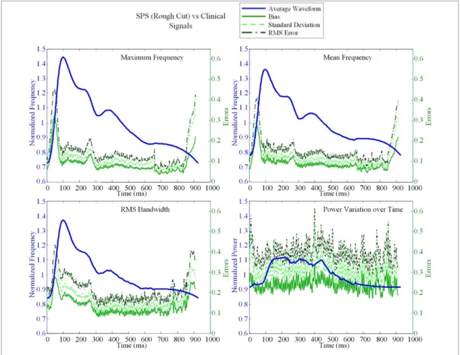
Figure 3.29 – SPS method with rough delimitation: average waveforms errors versus clinical

waveforms. ...86

Figure 3.30 – SPS method with rough delimitation: some feature points from clinical waveforms versus the average waveforms. The feature points considered are minimum systolic (D), peak systole (S), diastolic notch (N), and mean value (M)...87

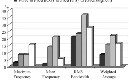
Figure 3.31 – RMSE normalized to the average for all methods and obtained when comparing the average waveforms with the waveforms from clinical signals. ...89

Figure 3.32 – Percentage bias for clinical variables obtained when comparing the average waveforms with the waveforms from clinical signals...89

Figure 3.33 – Percentage bias observed from the comparison between the average waveforms and the waveforms from clinical signals for the Pulsatility Index. ...90

Figure 3.34– Percentage bias observed from the comparison between the average waveforms and the waveforms from clinical signals for the Pourcelot’s Resistance Index. ...90

Figure 3.35 – Percentage bias observed from the comparison between the average waveforms and the waveforms from clinical signals for the acceleration. ...91

Figure 3.36– Percentage bias observed from the comparison between the average waveforms and the waveforms from clinical signals for the Spectral Broadening Index...91

Figure 3.37 – Filter modulated with the average waveforms. ...92

Figure 3.38 – Spectral representation of three clinical cardiac cycles and three simulated signals (both randomly selected). ...93

Figure 3.39 – Representation of the reference waveforms against the average waveforms from 100 simulated signals. ...94

Figure 3.40 – Bias achieved while comparing the reference waveforms with the average waveforms from 100 simulated signals. ...95

Figure 4.1 – Methods and signals used in this chapter. ...99

Figure 4.2 – STFT ...102

Figure 4.3 – STMC...110

Figure 4.4 – Scheme for determining the time-frequency spectrum, using the concept of time-frequency distribution [Forsberg et al., 1999]...112

Figure 4.5 – Correlation coefficients between the window length and the averaged bias obtained with the application of STFT to estimate the four spectral parameters. The results were obtained using simulated signals with and without noise. ...118

Figure 4.6 – Correlation coefficients between the percentage of windows overlap and the averaged bias obtained with the application of STFT to estimate the four spectral parameters. The results were obtained using simulated signals with and without noise. ...118

Figure 4.7 – Correlation coefficients between the window length and the averaged bias obtained with the application of STMC to estimate the four spectral parameters. The results were obtained using simulated signals with and without noise. ...121

(16)

Figure 4.8 – Correlation coefficients between the percentage of windows overlap and the averaged bias obtained with the application of STMC to estimate the four spectral parameters. The results were obtained using simulated signals with and without noise. ...121 Figure 4.9 – Correlation coefficients between the order of the autoregressive model and the averaged bias obtained with the application of STMC to estimate the four spectral parameters. The results were obtained using simulated signals with and without noise. ...122 Figure 4.10 – Correlation coefficients between the windows length and the averaged bias obtained with the application of DCWD to estimate the four spectral parameters. The results were obtained using simulated signals with and without noise. ...125 Figure 4.11 – Correlation coefficients between the percentage of windows overlap and the averaged bias obtained with the application of DCWD to estimate the four spectral parameters. The results were obtained using simulated signals with and without noise...125 Figure 4.12 – Correlation coefficients between the range from which the time index autocorrelation function is computed and the averaged bias obtained with the application of DCWD to estimate the four spectral parameters. The results were obtained using simulated signals with and without noise...126 Figure 4.13 – Correlation coefficients between the scaling factor and the averaged bias obtained with the application of DCWD to estimate the four spectral parameters. The results were obtained using simulated signals with and without noise. ...126 Figure 4.14 – Most favourable bias obtained with the estimation of the four spectral parameters with the three estimators. In the graph, Mf stands for maximum frequency, fm for mean frequency, bd for rms bandwidth and pv for power variation over time, and All for considering all parameters equally relevant for the assessment of the method...129 Figure 4.15 – Performance of the spectral estimation methods with the different spectral parameters for three levels of SNR. The smaller the percentage of bias, the better the estimation...129 Figure 4.16 – Performance of the estimators when a good estimation of the maximum frequency and power variation or of the mean frequency and power variation is required. ...130 Figure 5.1 – Main methods and signals used in this chapter. ...133 Figure 5.2 – Impact of Avl on MEP, for several values of L. ...135

Figure 5.3 – Variation of the embolic time duration with the embolic power, for a constant velocity and emboli lengths of a) SE=1mm, a) SE=5mm, and a) SE=10mm. ...137

Figure 5.4 – Variation of the time during which an embolus is observable with respect to embolus velocity and the axial sample volume length considered. ...138 Figure 5.5 – Representation of the independent samples of mean frequency (top) and rms bandwidth (bottom) waveforms. ...140 Figure 5.6 – Generation of an MCA Doppler blood flow signal with embolus...143 Figure 5.7 – Signal with S_E =770µm simulated with sine amplitude modulation on the left side, and the same signal without amplitude modulation on the left. ...144 Figure 5.8 – Velocities and localization of emboli...145 Figure 5.9 – Signals with S_E longer than 1mm, and without sine amplitude modulation. ...146

(17)

Figure 5.10 – First case study: Estimated MEP (maximum power) obtained with time-domain processing. The upper bar represents the expected MEP values, the right bar represents the colour scales. ...149 Figure 5.11 – First case study: Estimated MEP (mean power) obtained with time-domain processing. The left bar represents the colour scales...150 Figure 5.12 – First case study: Estimated MEP (maximum power) obtained with time-domain processing,

Avl=1mm, and a threshold for detection of 15dB...151

Figure 5.13 – First case study: Estimated MEP (maximum power) obtained with time-domain processing,

Avl=10mm, a threshold for detection of 15dB...151

Figure 5.14 – First case study: Total number of false negatives found for the 10 values of Avl using

time-domain processing with a threshold for detection of 15dB. ...152 Figure 5.15 – First case study: Estimation of the velocities of the emboli using time-domain analysis for an Avl=1mm. ...153

Figure 5.16 – First case study: Estimation of the velocities of the emboli using time-domain analysis for an Avl=10mm. ...154

Figure 5.17 – First case study: Estimation of the velocities of the emboli using time-domain analysis for an Avl=1mm, considering a threshold for detection 15dB...155

Figure 5.18 – First case study: Estimation of the velocities of the emboli using time-domain analysis for an Avl=10mm, considering a threshold for detection of 15dB. ...155

Figure 5.19 – First case study: Estimation of the SVL of the emboli using time-domain analysis for an

Avl=1mm, considering a threshold for detection of 15dB. ...156

Figure 5.20– First case study: Estimation of the SVL of the emboli using time-domain analysis for an

Figure 5.21 – First case study: Estimated MEP (maximum power) obtained with the STFT. The upper bar represents the expected MEP values, the right bar represents the colour scales...157 Figure 5.22 – First case study: Estimated MEP (mean power) obtained with the STFT. The left bar represents the colour scales. ...158 Figure 5.23 – First case study: Estimated MEP (maximum power) obtained with time-domain processing,

Avl=1mm, and a threshold for detection of 15dB...158

Figure 5.24 – First case study: Estimated MEP (maximum power) obtained with the STFT, Avl=10mm, a

threshold for detection of 6dB...159 Figure 5.25 – First case study: Total number of false negatives found for the 10 values of Avl using the

STFT with a threshold for detection of 6dB...159 Figure 5.26 – First case study: Estimation of the velocities of the emboli using the STFT for an

Avl=1mm. ...160

Figure 5.27 – First case study: Estimation of the velocities of the emboli using the STFT for an

Avl=10mm. ...161

Figure 5.28 – First case study: Estimation of the velocities of the emboli using the STFT for an Avl=1mm,

considering a threshold for detection 6dB...161 Figure 5.29 – First case study: Estimation of the velocities of the emboli using the STFT for an

(18)

Figure 5.30 – First case study: Estimation of the SVL of the emboli the STFT for an Avl=1mm,

considering a threshold for detection of 6dB...163 Figure 5.31– First case study: Estimation of the SVL of the emboli using the STFT analysis for an

Figure 5.32 – Second case study: Estimated MEP (maximum power) obtained with time-domain processing. The upper bar represents the expected MEP values, the right bar represents the colour scales. ...165 Figure 5.33 – Second case study: Estimated MEP (mean power) obtained with time-domain processing. The left bar represents the colour scales...165 Figure 5.34 – Second case study: Estimated MEP (maximum power) obtained with time-domain processing, Avl=10mm, a threshold for detection of 15dB...166

Figure 5.35 – Second case study: Total number of false negatives found for the 10 values of Avl using

time-domain processing with a threshold for detection of 15dB. For each Avl the total number of emboli

was 1400...166 Figure 5.36 – Second case study: Estimation of the velocities of the emboli using time-domain analysis for an Avl=1mm...167

Figure 5.37 – Second case study: Estimation of the velocities of the emboli using time-domain analysis for an Avl=10mm...168

Figure 5.38 – Second case study: Estimation of the velocities of the emboli using time-domain analysis for an Avl=10mm, considering a threshold for detection of 15dB...168

Figure 5.39 – Second case study: Estimation of the SVL of the emboli using time-domain analysis for an

Figure 5.40– Second case study: Estimation of the SVL of the emboli using time-domain analysis for an

Figure 5.41 – Second case study: Estimated MEP (maximum power) obtained with the STFT. The upper bar represents the expected MEP values, the right bar represents the colour scales. ...170 Figure 5.42 – Second case study: Estimated MEP (mean power) obtained with the STFT. The left bar represents the colour scales. ...171 Figure 5.43 – Second case study: Estimated MEP (maximum power) obtained with the STFT, Avl=10mm,

a threshold for detection of 6dB. ...171 Figure 5.44 – Second case study: Total number of false negatives found for the 10 values of Avl using the

STFT with a threshold for detection of 6dB. For each Avl the total number of emboli was 1400. ...172

Figure 5.45 – Second case study: Estimation of the velocities of the emboli using the STFT for an

Avl=1mm. ...172

Avl=10mm. ...173

Figure 5.48 – Second case study: Estimation of the SVL of the emboli the STFT for an Avl=1mm,

(19)

Figure 5.49– Second case study: Estimation of the SVL of the emboli using the STFT analysis for an

Figure 6.1 – Time Frequency representation of a simulated MCA Doppler signal plotted with the estimated normalized power variation over time. The spectral estimator was STFT with 20ms windows and 50% of overlapping...178 Figure 6.2 – Time-frequency representation of a simulated ES plotted with the estimated normalized power variation over time. The background signal is the same that was represented in Figure 6.1, the seven emboli are localized according to Figure 5.8. The effective axial length of the emboli is 10µm and the MEP is 6.5dB. The sample volume length of the probe was considered to be 1cm. ...179 Figure 6.3 – Time-frequency representation of a simulated ES plotted with the estimated normalized power variation over time. The background signal is the same that was represented in Figure 6.1, the seven emboli are localized according to Figure 5.8. The effective axial length of the emboli is 700µm and the MEP is 8dB. The sample volume length of the probe was considered to be 1cm. ...179 Figure 6.4 – Synthetic signal from carotid artery ...181 Figure 6.5 – Maximum frequency from a simulated Doppler signal in grey and the number of times that a sample with no significant information is calculated in black (q), when all the points in the time-domain signal are used for spectral estimation...181 Figure 6.6 – Maximum frequency from a simulated Doppler signal in grey and the number of times that a sample with new information is not calculated in black (q), when redundant information is undesired..182 Figure 6.7 – Maximum frequency from a simulated Doppler signal in grey and the number of times that a sample with the same information is calculated in black (q), when no significant information is missed183 Figure 6.8 – Maximum frequency from a simulated Doppler signal in grey and the number of times that important information is considered (q) in black. ...184 Figure 6.9 – Carotid artery synthetic Doppler signal spectral representation, considering the adaptive overlapping...184 Figure 6.10 – Carotid artery synthetic Doppler signal spectral representation, considering a constant overlapping...185 Figure 6.11 – MCA clinical Doppler signal spectral representation, considering the adaptive overlapping...186 Figure 6.12 – MCA clinical Doppler signal spectral representation, considering a constant overlapping186 Figure 6.13 – MCA clinical Doppler signal spectral representation, considering the adaptive overlapping and increased spatial resolution (5mm). ...187 Figure 6.14 – MCA clinical Doppler signal spectral representation, considering the adaptive overlapping and increased spatial resolution (1mm). ...187 Figure 6.15 – First case study: Estimated MEP (maximum power) obtained with the SF-STFT. The upper bar represents the expected MEP values, the right bar represents the colour scales. ...190 Figure 6.16 – First case study: Estimated MEP (mean power) obtained with the SF-STFT. The left bar represents the colour scales. ...190 Figure 6.17 – First case study: Estimated MEP (maximum power) obtained the SF-STFT, Avl=1mm, and a

(20)

Figure 6.18 – First case study: Estimated MEP (maximum power) obtained with the SF-STFT,

Figure 6.19 – First case study: Total number of false negatives found for the 10 values of Avl using the

SF-STFT with a threshold for detection of 6dB. For each Avl the total number of emboli was 3360...192

Figure 6.20 – First case study: Estimation of the velocities of the emboli using the SF-STFT for an

Avl=1mm. ...193

Avl=10mm. ...193

Avl=1mm, considering a threshold for detection 6dB. ...194

Avl=10mm, considering a threshold for detection of 6dB, and double space resolution...195

Figure 6.25 – First case study: Estimation of the SVL of the emboli the SF-STFT for an Avl=1mm,

considering a threshold for detection of 6dB...196 Figure 6.26 – First case study: Estimation of the SVL of the emboli using the SF-STFT for an Avl=10mm,

considering a threshold for detection of 6dB...197 Figure 6.27 – First case study: Estimation of the SVL of the emboli using the SF-STFT with double resolution for an Avl=10mm, considering a threshold for detection of 6dB...197

Figure 6.28 – Second case study: Estimated MEP (maximum power) obtained with the SF-STFT. The upper bar represents the expected MEP values, the right bar represents the colour scales. ...198 Figure 6.29 – Second case study: Estimated MEP (mean power) obtained with the SF-STFT. The left bar represents the colour scales. ...198 Figure 6.30 – Second case study: Estimated MEP (maximum power) obtained with the SF-STFT,

Figure 6.31 – Second case study: Total number of false negatives found for the 10 values of Avl using the

SF-STFT with a threshold for detection of 6dB. For each Avl the total number of emboli was 3360...199

Figure 6.32 – Second case study: Estimation of the velocities of the emboli using the SF-STFT for an

Avl=1mm. ...200

Avl=10mm. ...200

Avl=10mm, considering a threshold for detection of 6dB, and double space resolution...201

Figure 6.36 – Second case study: Estimation of the SVL of the emboli the SF-STFT for an Avl=1mm,

considering a threshold for detection of 6dB...202 Figure 6.37 – Second case study: Estimation of the SVL of the emboli using the SF-STFT for an

(21)

Figure 6.38 – Second case study: Estimation of the SVL of the emboli using the SF-STFT with double resolution for an Avl=10mm, considering a threshold for detection of 6dB...203

Figure 6.39 – First case study: amount of missed emboli for each A_vl for time-domain approach, STFT, and SF-STFT with simple and double resolution. ...204 Figure 6.40 – Second case study: amount of missed emboli for each A_vl for time-domain approach, STFT, and SF-STFT with simple and double resolution...205 Figure 7.1 – Normalized errors obtained with the STFT for the average of different windows length. MF stands for maximum frequency, fm for mean frequency and pv for power variation. The circles indicate the minimum errors. ...208

Figure 7.2 – Ratios of the average minimum MEPs that allow embolic detection and avoid false-positives...209

Figure 7.3 – Relationship between the estimated SVL with time domain processing and with the spectral estimation methods...210 Figure 7.4 – Comparison of the accuracy on estimating the SVL of emboli using and not using the correction factor. ...211

(22)

TABLES

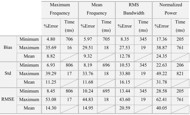
Table 2.1 – Studies on the MCA diameter ...20 Table 2.2 – Blood cells [Evans, McDicken, 2000]...22 Table 2.3 – Blood Properties. ...23 Table 3.1 – Choice of the capture window to be used on PFS algorithm (values considered for neonatal blood flow in cerebral arteries [Evans, 1988]) ...48 Table 3.2 – Description of the feature points for common carotid artery's maximum velocity waveform [Holdsworth et al., 1999]...49 Table 3.3 – Description of the feature points for middle cerebral artery spectral parameters waveform when clinical data is considered. ...52 Table 3.4 – Heart rates of the clinical signals...56 Table 3.5 – Values of the parameters to use on the ECG signals division (first approach)...60 Table 3.6 – Parameters used to divide ECG on each file...60 Table 3.7 – Description and first approach to the values of the parameters to be used in the PFS ...61 Table 3.8 – Parameters used to find pulse-foot of the cycles on each file...62 Table 3.9 – First approach to initial values of the parameters for rough division of spectral waveforms. 63 Table 3.10 – Parameters used for the rough division of the signals from each file. ...63 Table 3.11 – Parameters used to determine feature points ...65 Table 3.12 – Values used to determine the feature points ...66 Table 3.13 – Adapted WFA: Minimum, maximum and mean percentage errors between the average and clinical waveforms, and their time of occurrence...74 Table 3.14 – Adapted WFA: percentage errors for clinical variables obtained from the comparison of clinical waveforms with average waveforms. ...76 Table 3.15 – ECG based delimitation: bias between average waveforms when built with signals set in-phase and with signals obtained directly from cut (signals with expanded cycles)...80 Table 3.16 – PFS based delimitation: bias between average waveforms when built with signals set in-phase and with signals obtained directly from cut (signals with expanded cycles)...80 Table 3.17 – SPS method with ECG delimitation: Minimum, maximum and mean percentage errors between the average and clinical waveforms, and their time of occurrence...82 Table 3.18 – SPS method with ECG delimitation: percentage errors for clinical variables obtained from the comparison of clinical waveforms with average waveforms...83 Table 3.19 – SPS method with PFS delimitation: Minimum, maximum and mean percentage errors between the average and clinical waveforms, and their time of occurrence...84

(23)

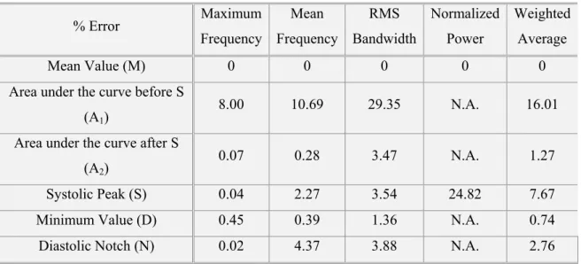
Table 3.20 – SPS method with PFS delimitation: percentage errors for clinical variables obtained from the comparison of clinical waveforms with average waveforms...85 Table 3.21 – SPS method with rough delimitation: Minimum, maximum and mean percentage errors between the average and clinical waveforms, and their time of occurrence...87 Table 3.22 – SPS method with rough delimitation: percentage errors for clinical variables obtained from the comparison of clinical waveforms with average waveforms...88 Table 3.23 – Minimum, maximum and mean percentage errors for the average waveforms from 100 simulated signals relatively to the reference waveforms. ...96 Table 4.1 – Some desirable properties of the time-frequency distributions and the corresponding kernel restrictions [Jeong,Williams,1992a]. ...113 Table 4.2 – Ranges where the errors obtained from the STFT estimation can be found...119 Table 4.3 – STFT optimal parameters for three levels of SNR (Win L. represents the window length in terms of discrete bins). ...120 Table 4.4 – Ranges where the errors obtained from the STMC estimation can be found. ...123 Table 4.5 – STMC optimal parameters for three levels of SNR (Win L. represents the window length in terms of discrete bins). ...124 Table 4.6 – Ranges where the errors obtained from the DCWD estimation can be found. ...127 Table 4.7 – DCWD optimal parameters for three levels of SNR (Win L. represents the window length in terms of discrete bins). ...128 Table 5.1 – Values used to generate the scenarios of the first case study ...146 Table 5.2 – Values used to generate the scenarios of the second case study...147 Table 5.3 – L codes for the first case study ...148 Table 5.4 – L codes for the second case study...164 Table 7.1 – Description of the files with clinical signals...206

(24)

ACRONYMS AND SYMBOLS

a(m) Parameters of the AR model

A(t) Amplitude of x(t)

A(z) z transform of the AR branch of an ARMA model

ab(m) AR backward linear prediction coefficient

ACF Autocorrelation function

ACS Autocorrelation sequence

AE Amplitude of the signal of the embolus

af(m) AR forward linear prediction coefficient

AR Autoregressive

ARMA Autoregressive moving average

ARMC Autoregressive modified covariance

Avl Axial length of the sample volume

B(f) Amplitude of the signal X(f)

b(m) Parameters of the MA model

B(z) z transform of the MA branch of an ARMA model

BCSb Backscattering cross-section of an erythrocyte

Bd Rms half bandwidth

bf(t) Rms bandwidth function

bt(t) Bandwidth of time varying filter

c Velocity of sound

C(t,f) MGM straight line

CW Continuous wave Doppler

CWD Choi-Williams Distribution

cxx(τ) Co-variance function of the process x(t)

d(t,f) vertical distances between Г(t,f) and C(t,f)

(25)

DE Duration of the ES

DFT Discrete Fourier transform

E Total energy

eb(n) Backward linear prediction error

ECG Electrocardiogram

ef(n) Forward linear prediction error

EN Window power density

ES Embolic Signal

f Frequency index

fd Doppler frequency

fE Mean frequency of the ES

FFT Fast Fourier transform

FIR Finite impulse response

fL Low frequency for MGM

fm Mean frequency

fm(t) Mean frequency function

fMAX(t) Measured maximum frequency function

fn Normalized frequency

fr Received frequency

fs Sampling frequency

ft Transmitted frequency

FT Fourier transform

h(t) Linear causal filter

h(t,ς) Time-varying filter

H(z) z domain transfer function

Hae Haematocrit

hbr Theoretical heart rate

k Discrete frequency index

KD Predetermined part of the Doppler equation

kmax(t) Registered maximum frequency

L Ratio between power of the embolus and power per unit of Avl

M CWD range for autocorrelation

(26)

MCA Middle cerebral arteries

MEP Measured embolic power

Mf Maximum frequency

MGM Modified geometric method

n Discrete time index

N Window length

Nc Number of cardiac cycles

Nhc Number of complete half cycles

nRI Refractive index

p Number of poles of the ARMA model

P(f) Power spectral density

P(f,t) Power spectral density in time-frequency domain

p(t) Power variation over time function

PAR(f,t) AR power spectrum

PB Power backscattered by blood

PE Power backscattered by the embolus

PFS Pulse-foot-seeking algorithm

PN Power of noise

PRF Pulse repetition frequency

PSA Phase shift algorithm

PSD Power spectrum density

pv Power variation over time

PW Pulse wave Doppler

q Number of zeros of the ARMA model

r Correlation coefficient

R’x(t,τ) Generalized time-indexed autocorrelation function

r’xx(τ) Autocorrelation temporal mean of the process x(t)

RF Radio-frequency

rgauss(t) Random Gaussian variable function

rms Root mean square

RMSE Root mean square error

rn(t) White Gaussian noise signal

(27)

Rx(t,τ) Instantaneous autocorrelation function

Rxx Autocorrelation matrix

rxx(τ) Autocorrelation of the process x(t)

rxy(τ) Cross-correlation between the processes x(t) and y(t)

s Axial space

SE Effective axial length of the embolus

SF Space-frequency

SF-DCWD Space-Frequency Discrete Choi-Williams Distribution

SF-STFT Space-frequency Short Time Fourier Transform

SF-STMC Space-Frequency Short Time Modified Covariance

SNR Signal to noise ratio

SPS Sequential Phase Shift Averaging

STFT Short Time Fourier Transform

STMC Short Time Modified Covariance

SVL Sample volume length

t Continuous time index

T Period

TCD Transcranial Doppler

TFD Time-frequency distribution

tg(f) Group delay

Ts Sampling period

u(t) Spectral parameter variation over time

U(t) Deterministic component of u(t)

u'(t) Random component of u(t)

us(t) Spectral parameter variation over independent samples

v Velocity

v(t) ARMA input sequence

V(t) Maximum velocity at time t

vE Velocity of the embolus

VHM Averaged diastolic velocity

Vm Lowest maximum velocity in the signal

VM Highest maximum velocity in the signal

(28)

Volc Average volume of one erythrocyte

w SF velocity weighting factor

w(t) Window function

wE(t) Embolus amplitude weighting factor

WF Wang and Fish simulator

WFA Waveform main features averaging

Wpack Packing factor

WSS Wide sense stationary process

X(f) Spectral representation of the signal x(t)

x(t) Generic time domain discrete signal

X(z) z transform of x(n)

xb(n) Backward linear prediction of x(n)

xb(t) Blood signal

xD(t) Direct flow in Doppler ultrasound signal

xe(t) Signal of the embolus

xf(n) Forward linear prediction of x(n)

xF(t) Phase component of xD(t)

xI(t) Complex component of x(t)

xQ(t) Quadrature component of xD(t)

xR(t) Real component of x(t)

xw(t) Windowed signal

yAM(t) Amplitude modulation function

yFM(t) Frequency modulation function

βe Adiabatic compressibility of erythrocytes

βp Adiabatic compressibility of plasma

Γ(t,f) Integrated Doppler power spectrum

∆E Fractional energy

∆s Axial space resolution

∆T Bounded time period

∆t Time cell

∆ω Frequency cell

φ(ξ,τ) TFD kernel function

(29)

θr Ultrasound reflection angle

θR Ultrasound refraction angle

λ Wavelength

µx Mean value of the process x(t)

ξ Frequency lag

ρ Mean squared error

ρb Mean squared backward linear prediction error

ρe Density of blood

ρf Mean squared forward linear prediction error

ρp Density of plasma

σ CWD scaling factor

σx Standard deviation of the process x(t)

σx2 Variance of the process x(t)

τ Time lag

υ Measure of the size of an aggregate scattering unit

φ(t) Phase of the signal x(t)

Φ(t) Deterministic phase of the Doppler signal

Φbs Backscattering coefficient of blood

ψ(f) Phase of the signal X(f)

Ψ(t,τ) TFD autocorrelation domain kernel

ω Angular frequency

(30)

1

1 I

I

N

T

R

O

D

U

C

T

I

O

N

1

1. .1

1 MO

M

OT

TI

IV

VA

A

TI

T

IO

ON

N

Recent technological developments together with the emergence of new diseases incentive the association of engineering and medicine areas to synergistically search the solution of clinical problems. The work developed in these areas leads to methods of higher accuracy in diagnosis, and encourages research aiming the solution of new challenges. Developments that have occurred in Doppler ultrasound instrumentation are an example of the successful application of engineering in medical vascular diagnosis.

Clinical Doppler instrumentation and the corresponding mathematical models became particularly relevant tools, because they allow the use of non-invasive methods in the measurement of blood flow characteristics.

The study of blood flow has been an important area of research both in medicine and in engineering. This research field includes, among other goals, the detection, and characterization of emboli in the cerebral circulation. In particular, transcranial Doppler (TCD) ultrasound instrumentation provides the assessment of blood flow information from intracranial arteries, namely from middle cerebral arteries (MCA), where cerebral embolic events can be observed.

This issue is especially relevant because cardiovascular diseases are the major cause of mortality in Portugal, as well as in the rest of Europe. Ischemic stroke, predominantly due to cerebral embolism [Zuillen et al., 1998], is one of the most important disorders, highly contributing to these statistics. The accurate detection and classification of emboli in brain blood circulation might help the prevention of such strokes.

(31)

Nowadays, many clinical and hospital units are provided with TCD instrumentation. These devices enable emboli detection, but still present some difficulties in identifying micro-emboli.

Correct characterisation of blood flow and cerebral emboli by TCD instrumentation depends on the precision obtained by the spectral estimation process. Most TCD equipment uses conventional spectral estimation methods based on the application of Short Time Fourier Transform (STFT). STFT present well identified limitations might lead to inaccurate quantitative measurements especially when small embolus detection is required.

Several published studies have reported the improvement in blood flow spectral estimation with methods other than the STFT. Most of these studies have used simulated Doppler ultrasound signals to test the alternative spectral estimators, and several arteries were analysed [Ruano, 1992] [Cardoso et al., 1996a] [Matos et al., 2000] [Guo et al., 1994] [Leiria, 2000] [García-Nocetti et al., 2001].

Detection and classification of embolic events in blood have been associated with time-domain processing and with time-frequency processing. The study and development of alternative estimators can help the choice of the best approach to process embolic signals (ES). Some studies on this subject can be found in [Fan, Evans, 1994], [Guetbi et al., 1997], [Girault et al., 2000], [Smith et al., 1996], [Smith et al., 1997], [Smith et al., 1998] and [Furui et al., 1999].

Although techniques allowing ultrasonic emboli detection and characterisation have been reported in the literature, these reports are scarce and do not convey a unique approach.

ESs are very complex and demand optimised methods and methodologies. The work hereby described envisages overcoming these issues and presents a structured approach to the assessment of blood flow, including, but not being restricted to, the detection and classification (characterisation) of emboli.

1

1. .2

2 GO

G

OA

AL

LS

S

The ultimate goal of this work is the improvement of emboli characterization in the MCA, when transcranial Doppler ultrasound instrumentation is employed. The strategy planned to reach this target includes three intermediate goals:

(32)

• The development of a MCA Doppler ultrasound signals simulator, with and without embolic occurrences. This will provide a reference signal for blood flow characterization through the analysis and development of spectral estimation methods;

• The statistical evaluation of time-frequency estimators. The simulated

signals will be used as reference signals to enable the spectral estimators’ assessment in terms of precision and accuracy of spectral parameters considered relevant for clinical diagnosis;

• Finally, the performance evaluation of the estimator previously identified

when applied to real clinical signals; its ability to detect and classify emboli will be assessed.

1

1. .3

3 TH

T

HE

ES

SI

IS

S

O

OU

U

TL

T

LI

IN

NE

E

The research work developed is organized into eight chapters.

The present chapter provides a brief overview of the thesis outline and the motivation of these studies. The major contributions of this research work are also summarized on this chapter.

Chapter 2 reviews general issues related to the analysis of spectral ESs. This chapter includes a description of Doppler ultrasound instrumentation, anatomy and blood composition, mathematical characterization of Doppler ultrasound blood flow signals, and the state of art of embolic characterization and detection.

Accurate spectral representation of ESs requires knowledge of the appropriate spectral estimator to be applied to the blood signal when it is free of emboli in order to enable differentiating the spectral properties when emboli are present. Therefore, chapters 3 and 4 are concerned with embolic free blood flow signals and the description of the study dedicated to these spectra.

Chapter 3 describes the simulation of embolic free blood flow signals in MCA. The chapter starts by justifying the use of simulated signals, basing the justification on theoretical issues and revising the main Doppler signals simulated reported in the bibliography. The simulator adopted in the current work is then presented. Characterization of MCA signals’ spectra and the description of the main spectral parameters and clinical indicators are described. An innovative algorithm for averaging Doppler blood flow parameters is reported on this chapter. The new algorithm was

(33)

developed based on two other existing methods (published in literature) but taking into account the MCA characteristics so that the averaging procedure could be obtained with better performance and considering other reference spectral parameters than the maximum frequency. Practical work is then reported, including the description of tests and results obtained when evaluating the modified averaging methods. Finally, the identification and description of the averaged parameters that will constitute the reference spectral parameters signals employed as inputs to the simulator are described, followed by the evaluation of the accuracy of the signals simulator.

Spectral analysis is addressed in Chapter 4. This chapter includes the description of the spectral estimators STFT, Choi-Williams Distribution (CWD) and Short Time Modified Covariance (STMC). The discrete formulation and application of these methods to simulated MCA blood flow signals is described. The results’ evaluation according to the relevant spectral parameters is also accomplished leading to the choice of the best estimator. This chapter also includes a study on the relevance of each parameter on the performance of the method.

Chapter 5 reports the simulation and processing of ESs. An overview of the main features of emboli detection and characterization is followed by the description of the simulation process. The best-performed spectral estimator is compared to time-domain analysis results.

The results obtained and reported in the previous chapter, induced the development of a new method for spectral representation of Doppler signals, the space-frequency representation, described in Chapter 6. The mathematical formalization of the new method, its application to the simulated ESs, and its comparison with the STFT and time-domain processing are also included in Chapter 6.

Chapter 7 presents the results of the application of the statistical evaluation of STFT, time-domain processing and the space-frequency version of the STFT, to clinical signals.

In Chapter 8 general conclusions taken from this work are drawn. Guidelines for future work are also suggested.

(34)

Figure 1.1 – Practical work addressed in each chapter of the thesis.

1

1. .4

4 OR

O

RI

I

GI

G

IN

NA

AL

L

CO

C

ON

NT

TR

RI

IB

BU

UT

TI

IO

ON

NS

S

The main contributions of this thesis may be summarized as follows:

• Method and algorithm for representing a spectrogram in the space-frequency

domain

The mathematical formulation and computational implementation of an innovative space-frequency blood flow representation; Statistical accuracy of the proposed method overcomes the accuracy obtained with traditional and time-frequency methods.

• Methods and algorithms for simulating MCA ultrasound blood flow signals

and embolic signals

The development of a MCA Doppler ultrasound signal simulator, employing a new averaging algorithm, where the input data is able to accept clinical Doppler signals, including the variation of clinical ultrasound power spectra during the cardiac cycle; The simulator includes the possibility of adding to the MCA signals embolic events with user-defined time location and power spectral characteristics.

• Quantification of the influence of the spectral estimators parameters on the accuracy of the estimation

(35)

The spectral parameters accuracy and its influence on the general spectral estimator accuracy was studied; these influences were rated according to the grade of influence each parameter had on the global method performance; the study has been applied to both signals with emboli or emboli-free; These hierarchies enabled the definition of fine tuned MCA blood flow spectral estimators.

• Method and algorithm for computing the average signal from random

time-variable signals

The development of an innovative technique for averaging stochastic non-stationary signals, composed by consecutive segments with different lengths but similar periodic characteristics.

So far, these contributions were reported in:

Leiria Ana, Ruano M. G., Evans D. H., Blood Flow Signals

Characterization, 12th New England Doppler Conference, Artimino, Florence,

May 2003

Leiria Ana, Moura M. M. M., Ruano M. Graça, Time-Variable Blood Flow

Averaged Waveforms, Controlo 2004 - Sixth Portuguese Conference on

Automatic Control, Vol. 2, pp. 625-629, Faro, Portugal, June 2004

Leiria Ana, Moura M. M. M., Solano Julio, Ruano M. Graça, Evans David H., Middle Cerebral Artery Blood Flow: Accurate Time-Frequency Evaluation, Anais do IIICLAEB’2004/XIXCBEB’2004 - Conferência Latino-Americana de Engenharia Biomédica, pp. 1095-1098, João Pessoa, Brazil, September 2004

Leiria Ana, Moura M. M. M., Evans David H., Ruano M. Graça,

Time-Variable Blood Flow Averaged Waveforms, submitted to International Journal of

Systems Science, 1st October 2004

(36)

2

2 B

B

A

C

K

G

R

O

U

N

D

2

2. .1

1 IN

I

NT

TR

RO

O

DU

D

UC

CT

TI

IO

O

N

This chapter summarizes the fundamental issues related with the main subjects involved in spectral analysis of ESs: Doppler ultrasound, spectral analysis, and embolic analysis. The characterization of ultrasound waves and the concepts, techniques and methods associated with TCD ultrasound instrumentation are reviewed. A few anatomical aspects related to blood flow, such as the circulatory system, heart and blood vessels, are presented. Blood is described as the main source of information for Doppler ultrasound diagnosis. The Doppler signal is mathematically characterized and the procedures used to extract the required clinical information are outlined. Finally, the concepts related to embolic Doppler signals’ processing are exposed.

2

2. .2

2 DO

D

OP

PP

PL

LE

ER

R

U

LT

L

TR

RA

AS

SO

OU

UN

ND

D

Ultrasound is being increasingly employed for diagnosis purposes since it allows the visualisation of the interior of the human body. Ultrasound instrumentation exploiting the Doppler effect allows monitoring of the moving structures within the body, for example fetal movement and blood flow. TCD equipment, in particular, is used for identification of emboli in the MCA.

A wave is a movement of energy defined as a periodic repetition of a disturbance from a normal or equilibrium condition [Evans, McDicken, 2000].

A sound wave is a mechanical wave travelling through matter. The propagation of ultrasound is due to the action among the atoms in the medium. That action is

(37)

transmitted to other atoms, along with a loss of energy. This loss of energy determines the length the wave can travel within the medium.

Ultrasound is a sound wave with frequencies above the human audible range of frequencies, i.e., above 20 kHz. Diagnostic ultrasound devices emit ultrasound waves into the human body, and collect and analyse the echoes returned by the structures reached by the wave.

The piezoelectric effect and the interaction between the ultrasound wave and the medium are physical phenomena directly related to diagnostic ultrasound. The former allows controlling the ultrasonic wave and interpreting its echoes while the physical phenomena affect the interpretation of the returned echoes.

When some solids suffer a mechanical pressure, they produce small electric charges, the so-called piezoelectric effect. Therefore, the incidence of ultrasound waves on a piezoelectric crystal originates a transmission of electric impulses susceptible of being electronically processed.

This is a reversible effect since when some voltage is applied to a piezoelectric solid, it suffers a mechanical distortion, and accordingly, if an alternating current is applied to the crystal, the electric field will create oscillations (surface compression and rarefaction) and produce ultrasonic waves.

This property is very useful when applied to diagnostic ultrasound, and it is used to generate (inverse piezoelectric effect) and receive (piezoelectric effect) electronically controlled ultrasound waves (Figure 2.1).

Figure 2.1 – Piezoelectric effect and inverse piezoelectric effect

When the ultrasound waves enter the human body, three main phenomena occur and affect the posterior interpretation of the returned echoes. These are reflection, refraction, and absorption.

(38)

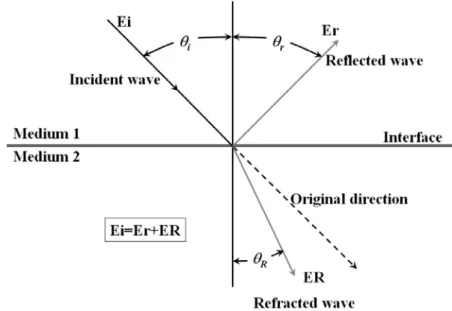
When a wave crosses a medium and reaches a plane interface, part of the wave is reflected and part is refracted.

Reflection occurs when ultrasound reaches a surface with small irregularities and walls with higher dimensions than the wavelength. In this case, the incidence angle (θ_i) and the reflection angle (θ_r) are the same [Evans, McDicken, 2000].

However, if the medium has discontinuities with lower or equal dimension than the wavelength of the ultrasound, some of that wave's energy will scatter in several directions, as illustrated in Figure 2.2. Those discontinuities may be caused by changes on density or compressibility of the medium.

Figure 2.2 – Scatter concept

Refraction and reflection are represented in Figure 2.3.