Bruno Miguel Faria do Vale
Development of a coextrusion system of
multifunctional filaments for the
production of high performance ropes
Bruno Miguel Faria do Vale
De velopment of a coe xtr usion sys tem of multifunctional filaments for t he pr
oduction of high per
for
mance r
opes
Dissertação de Mestrado
Ciclo de Estudos Integrados Conducentes ao
Grau de Mestre em Engenharia de Polímeros
Trabalho efetuado sob a orientação de
Professor Doutor João Miguel Nóbrega
Doutor Célio Bruno Pinto Fernandes
Mestre Fernando Eblagon
Bruno Miguel Faria do Vale
Development of a coextrusion system of
multifunctional filaments for the
production of high performance ropes
Escola de Engenharia
A
CKNOWLEDGMENTS
The execution of this MSc thesis was only possible due to the contribution and guidance of several people.
Firstly, I want to sincerely express my gratitude to my advisers Professor Doctor João Miguel Nóbrega, Doctor Célio Fernandes and Master Fernando Eblagon. To Professor Doctor João Miguel Nóbrega and Master Fernando Eblagon I want to thank for the guidance and support during this project and for making available all the resources needed to perform this MSc project. I thank to Doctor Célio Fernandes for the patience demonstrated in help me solving all the many problems and challenges faced and for the knowledge provided regarding the OpenFOAM® framework computational library.
I also want to thank to all the people in Lankhorst for the demonstrated sympathy and the knowledge provided.
In addition, I like to thank all my co-workers in Polymer Engineering Department of the University of Minho for the support and friendship. I want to highlight Ananth Rajkumar for providing the tool required to simulate the extrusion process and to António Abreu for providing the experimental results needed to validate the solvers used.
To my closest friends who accompanied me over these five years, especially to Miguel Coelho and Melisa Freitas, I am so grateful for all the support and friendship given to me.
Lastly but not least, I would like to express my gratitude to my family. I thank to my father Fernando, my mother Joana and my brother Rui for the support that they give to me, for the patient and for always believe in me. I also want to dedicate this thesis to my grandmother Maria, who sadly passed away, but I know that she is very proud and she will always guide me wherever she is.
v
A
BSTRACT
Due to the increasingly demand on performance, several products that were in the past manufactured using just one material, are nowadays designed to incorporate more than one. This allows to take advantage of the specific properties of each material employed, like mechanical, barrier, chemical resistance, etc. However, the difficulties to anticipate the flow of several rheologically complex materials inside the production tools, are significantly increased when more than one material flows in the same channel.
Based on the above, numerical modelling tools may play an important role to support the designer’s activity, especially when dealing with products for which there is no previous experience. This MSc project aims to evaluate the capability of using OpenFOAM® framework to support the design of coextrusion processing tools and to develop a new semi-industrial filament coextrusion die. The numerical code assessment was started with verification studies, where numerical results obtained with the OpenFOAM® framework code were compared with data available in the scientific literature. Subsequently the assessment was performed with two experimental case studies, corresponding to extrusion dies to produce simple and coextruded filaments. The results obtained show clearly that OpenFOAM® was able to capture several flow effects, namely the interface location, and thus seems to be adequate to support the design of coextrusion production tools. The final part of the work comprised the design of a semi-industrial filament coextrusion die capable of produce filaments with different formulations, at a relative wide range of mass flow rates, which was done with the support of the OpenFOAM® computational library.
Keywords
Filament, Coextrusion, Coextrusion Die Design, OpenFOAM®, Verification, Experimental
R
ESUMO
Devido à crescente procura de melhores propriedades, muitos produtos que no passado eram produzidos só com um material, são nos dias de hoje projetados para serem constituídos por mais do que um material. Este facto permite tirar partido de propriedades específicas de cada material utilizado, como propriedades mecânicas, barreira, resistência química, etc. Contudo, as dificuldades em antecipar o fluxo de vários materiais reologicamente complexos dentro das ferramentas de produção são significativamente aumentadas quando mais do que um material fluí no mesmo canal.
Baseado no anteriormente exposto, as ferramentas de modelação numérica podem desempenhar um papel importante no apoio à atividade do projetista, especialmente quando aplicadas em produtos nos quais não existe experiência prévia. Este projeto de mestrado pretende avaliar a capacidade em usar a libraria computacional OpenFOAM® no auxílio à conceção de ferramentas para o processo de coextrusão e em desenvolver uma nova cabeça de coextrusão de filamento semi-industrial. A avaliação do código numérico começou com estudos de verificação, conseguidos pela comparação de resultados obtidos através do OpenFOAM® com dados disponíveis na literatura cientifica. Subsequentemente a avaliação foi realizada para dois casos de estudo experimentais, correspondentes a cabeças de extrusão utilizadas para produzir filamentos simples e coextrudidos. Os resultados obtidos demonstram que a libraria computacional OpenFOAM® é capaz de capturar vários efeitos no fluxo, nomeadamente a localização da interface, parecendo assim adequado para auxiliar a conceção de ferramentas de coextrusão. A última tarefa do projeto consistiu na conceção de uma cabeça de coextrusão de filamentos semi-industrial capaz de produzir filamentos com diferentes formulações, numa relativa vasta gama de débitos mássicos, conseguida com a ajuda da libraria computacional OpenFOAM®.
Palavras-Chave
Filamento, Coextrusão, Conceção de Cabeças de Coextrusão, OpenFOAM®, Verificação,
Contents
Acknowledgments ... iii Abstract ... v Resumo ... vii List of Figures ... xi List of Tables ... xvList of Abbreviations and Acronyms ... xvii
Introduction ... 1
1.1 State of the art ... 1
1.1.1 Filament extrusion and coextrusion ... 1
1.1.2 Filament coextrusion die ... 4
1.1.3 Rheological defects ... 6
1.1.4 Interface distortions in coextrusion ... 9
1.1.5 The importance of Computer Aided Engineering in die design ... 11
1.1.6 OpenFOAM® ... 13
1.2 Motivation ... 15
1.3 Objectives ... 15
1.4 Thesis structure ... 16
Verification case – 2D coextrusion ... 17
2.1 Geometry generation ... 18
2.2 Mesh generation ... 19
2.3 Properties of the polymeric blends ... 22
2.4 Boundary conditions ... 24
2.5 Results and discussion ... 25
OpenFOAM® experimental assessment ... 33
3.1 Rheological models and properties of the blends ... 33
3.2 Extrusion of Monofilaments ... 37
3.2.1 Geometry and operating conditions ... 38
3.2.2 Mesh and boundary conditions ... 39
3.2.3 Results and discussion ... 42
3.3.1 Geometry and operation conditions ... 47
3.3.2 Mesh and boundary conditions ... 49
3.3.3 Results and discussion ... 52
Design of a semi industrial multifilament coextrusion die ... 63
4.1 Die constructive solution ... 63
4.2 Mesh and boundary conditions ... 67
4.3 Results and discussion ... 70
Conclusions and future work ... 91
5.1 Conclusions ... 91
5.2 Future work... 92
Bibliographic references ... 93
Appendixes ... 97
Appendix A – Developed flow in the more refined mesh created using blockMesh ... 97
Appendix B – Interface in cases with mesh created using blockMesh ... 97
Appendix C – Streamlines in cases with mesh created using blockMesh ... 98
Appendix D – Velocity profile and pressure field in Cases 3, 4 and 5 ... 99
L
IST OF
F
IGURES
Figure 1 - Scheme of a typical filament extrusion line adapted from (Giles, Wagner, & Mount, 2004). ... 2 Figure 2 - Scheme of the filament coextrusion line used by Glauß and his co-workers (Glauß et al., 2013). ... 4 Figure 3 - Cross section of a sheath-core filament. ... 5 Figure 4 - Monofilament coextrusion die used by Martins and his co-workers (Martins et al., 2014). ... 5 Figure 5 - Scheme of the rearrangement of the velocity profile at the die exit (Carneiro & Nóbrega, 2012). ... 7 Figure 6 - The most frequent forms of melt fracture (Rauwendaal, 2014). ... 7 Figure 7 - Illustration of die drool formation, accumulation and eventual removal by the extrudate (Carneiro & Nóbrega, 2012). ... 8 Figure 8 - Overall structure of OpenFOAM® (Greenshields, 2015). ... 14 Figure 9 - Schematic representation of the double-layer coextrusion die used by Hannachi and Mitsoulis (Hannachi & Mitsoulis, 1993) (all design measures are given in mm). ... 17 Figure 10 - Geometry obtained with the SolidWorks CAD software: a) frontal view; b) isometric view. ... 18 Figure 11 - Example of the eight vertices points that define one single block of the geometry. ... 19 Figure 12 - Meshes created with cfMesh: (a) coarser mesh (M1) and (b) more refined mesh (M4). ... 20 Figure 13 - Meshes created with blockMesh: (a) coarser mesh (M1) and (b) more refined mesh (M4). ... 21 Figure 14 - Rheological curves of the polymer blend P2 and P3 (Hannachi & Mitsoulis, 1993). ... 23 Figure 15 - Initial domain distribution used for all the computational runs: the red field represents the P2 mixture and the blue field represents the P3 mixture. ... 25 Figure 16 - Steady state flow for 2D coextrusion case study, for the more refined mesh created using cfMesh in: a) Case 1; b) Case 2; c) Case 3. ... 26 Figure 17 - Interface coordinates for Case 1 (mesh created using cfMesh). ... 27 Figure 18 - Interface coordinates for Case 2 (mesh created using cfMesh). ... 27
Figure 19 - Interface coordinates for Case 3 (mesh created using cfMesh). ... 28
Figure 20 - Interface coordinates for Case 1 (mesh created using blockMesh). ... 28
Figure 21 - Streamlines obtained by Hannachi and Mitsoulis (Hannachi & Mitsoulis, 1993).30 Figure 22 - Representation of the streamlines (coloured according with the velocity intensity) for the more refined mesh created using cfMesh in: a) Case 1; b) Case 2; c) Case 3. ... 31
Figure 23 - Viscosity curves using the Carreau model for Blend A. ... 35
Figure 24 - Viscosity curves using the Carreau model for Blend B. ... 35
Figure 25 - Viscosity curves using the Carreau model for Blend A and B at 230℃. ... 36
Figure 26 - 3D geometry of the extrusion die used in the extrusion process. ... 38
Figure 27 - Geometry of the extrusion die flow channel. ... 38
Figure 28 - Slice of the flow channel used in the simulations: (a) frontal view and (b) isometric view. ... 40
Figure 29 - Meshes used in the simulations of the extrusion of the filaments: (a) coarser mesh (M1) and (b) more refined mesh (M3). ... 41
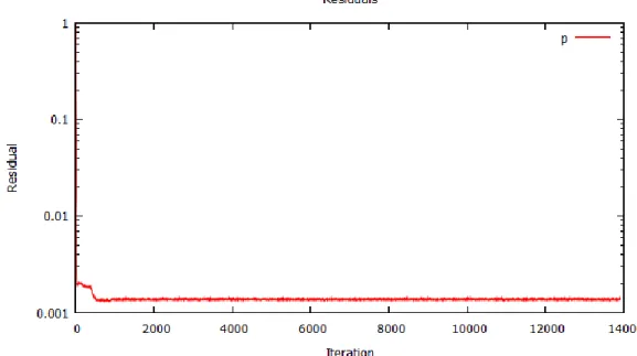
Figure 30 - Evolution of the residuals along the simulated time in the extrusion process. ... 42
Figure 31 - Pressure field predicted by the code along the die during the extrusion process of the Blend A (a) and Blend B (b). ... 44
Figure 32 - Velocity field predicted by the code along the die during the extrusion process of the Blend A (a) and Blend B (b). ... 44
Figure 33 - Temperature field predicted by the code along the die during the extrusion process of the Blend A (a) and Blend B (b). ... 45
Figure 34 - 3D model of the coextrusion die modules used to produce the multifunctional filaments. ... 47
Figure 35 - Geometry of the flow channels of the original coextrusion die. ... 47
Figure 36 - Geometry of the coextrusion die flow channels using Configuration 1. ... 48
Figure 37 - Geometry of the coextrusion die flow channels using Configuration 2. ... 48
Figure 38 - Meshes created using Configuration 2 geometry: (a) coarser mesh (M1) and (b) more refined mesh (M3). ... 50
Figure 39 - Interface between the two materials at the die exit at (a) 7 seconds and at (b) 9 seconds for configuration 1. ... 52
Figure 40 - Flow along one transversal section of the coextrusion die using configuration 1. 52 Figure 41 - Interface between the two materials at the die exit at (a) 7 seconds and at (b) 9 seconds for configuration 2. ... 53 Figure 42 - Flow along one transversal section of the coextrusion die using configuration 2. 53
Figure 43 - Evolution of the residuals along the simulated time in the coextrusion process. .. 54
Figure 44 - Location of the four points of the domain used. ... 55
Figure 45 - Interface location between the two materials at 2.5 seconds (a), at 4.5 seconds (b) and at 5.5 seconds (c). ... 56
Figure 46 - Pressure drop along the coextrusion die obtained with the more refined mesh. ... 56
Figure 47 - Pressure in function of the mesh cell size. ... 58
Figure 48 - Interface location at the outlet in each mesh used. ... 59
Figure 49 - Interface shape obtained using the extrapolated parameters. ... 61
Figure 50 - Microscopy picture of the produced filaments (Abreu, To be published). ... 61
Figure 51 - Assembly of all the components that composes the die that Lankhorst owns. ... 64
Figure 52 - Design of the multifilament coextrusion die channels for Solution 1. ... 64
Figure 53 - Design of the multifilament coextrusion die channels for Solution 2. ... 65
Figure 54 - Overall view of the 3D model of the designed die (a) and bottom view of the 3D model of the designed die (b). ... 66
Figure 55 - Typical geometry of the distributor used to create the mesh. ... 67
Figure 56 - Example of a typical mesh used in the simulations. ... 68
Figure 57 - Evolution of the residuals along the simulated time in the coextrusion process. .. 71
Figure 58 - Location of the four points of the domain used. ... 71
Figure 59 - Representation of the undeveloped flow at: (a) 1 second and (b) 4 seconds. ... 72
Figure 60 - Representation of the developed flow at: (a) 4.5 second and (b) 6 seconds. ... 73
Figure 61 - Distributor created in the first iteration: geometry (a) and flow of the blends in the distributor (b). ... 74
Figure 62 - Distributor created in the sixth iteration: geometry (a) and flow of the blends in the distributor (b). ... 74
Figure 63 - Representation of the distributor used in the design of the die ... 76
Figure 64 - Distributor created in the last iteration: geometry (a) and flow of the materials in the distributor (b). ... 76
Figure 65 - Interface location with an angle of 60° and 70° in the convergent channel of the die. ... 77
Figure 66 - Pressure drop in the two distributors in study: (a) with an angle of 60° and (b) with an angle of 70° in the convergent channel. ... 77
Figure 67 - Interface location and graphical representation of the equations for the Reference case. ... 80
Figure 69 - Velocity profile along the distributor in the Reference case. ... 83
Figure 70 - Pressure field along the distributor in the Reference case. ... 83
Figure 71 - Velocity profile along the distributor in Case 1. ... 83
Figure 72 - Pressure field along the distributor in Case 1. ... 84
Figure 73 - Interface location in Case 2: (a) rupture of the interface and (b) instabilities in the die parallel zone. ... 85
Figure 74 - Interface location and graphical representation of the equations for Case 3. ... 85
Figure 75 - Interface location and graphical representation of the equations for Case 4. ... 86
Figure 76 - Interface location and graphical representation of the equations for Case 5. ... 86
Figure 77 - Representation of the fully developed flow for the more refined mesh created using blockMesh in: a) Case 1; b) Case 2; c) Case 3. ... 97
Figure 78 - Interface coordinates for Case 2 (mesh created using blockMesh). ... 97
Figure 79 - Interface coordinates for Case 3 (mesh created using blockMesh). ... 98
Figure 80 - Representation of the streamlines for the more refined mesh created using blockMesh in: a) Case 1; b) Case 2; c) Case 3. ... 98
Figure 81 - Velocity profile along the distributor in Case 3. ... 99
Figure 82 - Pressure field along the distributor in Case 3. ... 99
Figure 83 - Velocity profile along the distributor in Case 4. ... 99
Figure 84 - Pressure field along the distributor in Case 4. ... 100
Figure 85 - Velocity profile along the distributor in Case 5. ... 100
Figure 86 - Pressure field along the distributor in Case 5. ... 100
Figure 87 - 2D drawing of the filament coextrusion die frame. ... 101
Figure 88 - 2D drawing of the module 1 of the filament coextrusion die. ... 102
Figure 89 - 2D drawing of the module 2 of the filament coextrusion die. ... 102
Figure 90 - 2D drawing of the module 3 of the filament coextrusion die. ... 102
Figure 91 - 2D drawing of the module 4 of the filament coextrusion die. ... 102
Figure 92 - 2D drawing of the seal module of the filament coextrusion die. ... 102
L
IST OF
T
ABLES
Table 1 - Relevant data for all the meshes generated with cfMesh. ... 20
Table 2 - Relevant data for all the meshes generated with blockMesh. ... 22
Table 3 - Rheological constants and density of the materials for the Carreau model. ... 24
Table 4 - Inlet velocities for the three cases documented in the paper. ... 25
Table 5 - 𝐿1 errors for the meshes created using cfMesh and blockMesh for the three case studies. ... 29
Table 6 - Rheological constants for the Carreau model. ... 34
Table 7 - Rheological constants for the Power Law model. ... 35
Table 8 - Relative content of blend materials and the properties calculated using the law of mixtures. ... 36
Table 9 - Values of the thermal diffusivity coefficient and the alpha for the Blend A and B. . 37
Table 10 - Inlet velocities of the Blend A and B in the extrusion process. ... 41
Table 11 - Evolution of the velocity and pressure values in three different points along the simulated time. ... 43
Table 12 - Pressures obtained using the simulations and experimentally in the same spot and the error between them. ... 46
Table 13 - Relevant information about the meshes created using Configuration 2. ... 51
Table 14 - Inlet velocities of the Blend A and B in the coextrusion process. ... 51
Table 15 - Evolution of the velocity and pressure values in four different points along the simulated time. ... 55
Table 16 - Values of pressure at the die inlet, in the missing section and the corrected pressure. ... 57
Table 17 - Constants of the ellipse equation for all meshes and the ones calculated using the Richardson extrapolation. ... 60
Table 18 - Relevant information about the example of a typical mesh used in the simulations. ... 69
Table 19 – Inlet velocities of the Blend A (inlet 2) and Blend B (inlet1) in the coextrusion process. ... 70
Table 20 - Evolution of the velocity and pressure values in four different points along the simulated time. ... 72
Table 22 - Shear rates and shear stresses developed in each of channel in all the processing conditions considered. ... 79 Table 23 - Constants of the ellipse and the circumference equations for the Reference case and for Case 1. ... 81 Table 24 - Minimum and maximum sheath thickness of the filament for the Reference case and for Case 1. ... 81 Table 25 - Minimum and maximum tolerance (radius) of the interface location in Reference case and Case 1. ... 82 Table 26 - Constants for the ellipse and circumference equations for Cases 3, 4, and 5. ... 87 Table 27 - Minimum and maximum thickness of the filament sheath for Cases 3, 4 and 5. ... 87 Table 28 - Minimum and maximum tolerance (radius) of the interface location in Cases 3, 4 and 5. ... 88
L
IST OF
A
BBREVIATIONS AND
A
CRONYMS
CAE – Computer Aided Engineering
CFD – Computational Fluid Dynamics
FVM – Finite Volume Method
HPC – High Performance Computing
OpenFOAM – Open Source Field Operation and Manipulation
I
NTRODUCTION
1.1 State of the art
1.1.1 Filament extrusion and coextrusion
The extrusion process allows the production of products usually with constant cross section. This process is applied in the processing of a wide range of materials, e.g. metal, food, chemicals substances (pharmaceutic industry) and plastic products (pipes, profiles, films, among others) (Gonçalves, 2013; Rauwendaal, 2014).
In the case of interest, which is the processing of polymeric materials, the extrusion can be subdivided in various sub techniques (pipe extrusion, profile extrusion, film extrusion and filament extrusion), which comprises specific post extrusion equipment, such as dies and calibrators (Gonçalves, 2013). The intrinsic properties of the polymers make them ideal to process by extrusion, because it is theoretically possible to obtain products with any cross section, at high production rates and quality. Thus they have been used to satisfy the constant demand of ever more complex products.
Since the main topic of this MSc project is the production of filaments, only the filament extrusion processing technique is going to be described in detail.
The filament extrusion technique is used to produce products that are employed to manufacture a wide range of objects that we use in our day life such as ropes, fishing lines, strings for racquets used in various sports, synthetic yarns, among several others (Giles, Wagner, & Mount, 2004).
A typical filament extrusion line is generally composed by an extruder, an extrusion die (mounted at the extruder exit), a water bath, godet rolls, draw ovens (heaters) and optionally a winding storage rolls. Figure 1 illustrates a typical filament extrusion line.
In this process the polymer pellets are fed to a hopper which by the action of the gravity force feeds the extruder (Gonçalves, 2013). The extruder contains one or more screws (for instance a multiscrew extruder) which rotate permanently and are responsible for the mixing, pressuring and transport of the polymeric material inside the barrel flow channel (Gonçalves, 2013). A group of heaters mounted along the extruder barrel, along with the viscous dissipation phenomena that happens when polymeric material is subjected to shearing forces, are responsible for generating the heat required to melt the polymer pellets. At the extruder outlet, the material is forced to pass through the die which transforms the circular flow from the extruder outlet into a flow with the required cross section (Gonçalves, 2013).
Frequently, between the extruder and the extrusion die a gear pump is used in order to provide a more controlled flow rate. Otherwise, due to the natural slight variations verified in processing conditions, the diameter of the filaments could vary and, thus affect negatively the product quality (Giles, Wagner, & Mount, 2004).
Subsequently, the extruded filaments are forced into a cooling bath (Ferreira et al., 2011; Giles, Wagner, & Mount, 2004). Exiting the cooling bath, the filaments are dried and passed throw godet rolls (the number of godet rolls used depends of the required draw forces) which control the speed and the drying of the filaments from the die until that point in the extrusion line (Ferreira et al., 2011; Giles, Wagner, & Mount, 2004). Between the first set of godet rolls and the second set, there is a draw oven which heats the filaments, in order to promote mobility to the polymer chains which makes it easier to orientate and elongate by the action of the second set of godet rolls (Giles, Wagner, & Mount, 2004). The second godet rolls presented in Figure 1, runs at a higher linear speed
Figure 1 - Scheme of a typical filament extrusion line adapted from (Giles, Wagner, & Mount, 2004).
than the first set, and this determines the stretch ratio developed inside the oven, which promotes the orientation of the polymer chains in the flow direction. The effectiveness of this orientation affects directly the filament mechanical strength (Ferreira et al., 2011; Giles, Wagner, & Mount, 2004). At the end of the extrusion line, the filaments are winded, using a method that varies with the product (for instance, textiles filaments are frequently winded in bobbins) (Giles, Wagner, & Mount, 2004).
Sometimes the intrinsic properties, or cost, of the polymeric material are inadequate to satisfy the required specifications for a given application. In those cases, it is common to combine two or more different materials, or the same material with different formulations, in order to obtain products with better properties formed by well-bounded layers of those materials (Giles, Wagner, & Mount, 2004; Rauwendaal, 2014; Riquelme, 1995). This variant of the extrusion technique is called coextrusion, and consists in extruding two or more materials simultaneously to obtain a product that combines the most favourable properties of its constituents.
The driving force for the development of the coextrusion process it is the need of obtaining even more cheaper, appealing and resistant products (Giles, Wagner, & Mount, 2004; Rauwendaal, 2014). In the case of the filament industry, this process has been applied in order to obtain filaments with more and more resistance (for instance, to manufacture high strength ropes), filaments with conductive properties (Glauß et al., 2013; Martins et al., 2014), optical fibres, among others.
The filament coextrusion line is quite similar to the filament extrusion line already illustrated in Figure 1, as it can be seen in Figure 2 that presents the filament coextrusion line (in this figure are missing the water bath and the draw oven, that most of filament coextrusion lines possess) used by Glauß and his co-workers (Glauß et al., 2013). In fact, the main differences between the extrusion and the coextrusion line, in almost all the known processes, are related to the die and to the fact that more than one extruder is used, as it can be verified when comparing a typical extrusion line with the experimental setups described in the works of Martins et al (Martins et al., 2014), Wang et al (Wang et al., 2013), Dooley (Dooley, 2002) and Glauß et al (Glauß et al., 2013).
Figure 2 - Scheme of the filament coextrusion line used by Glauß and his co-workers (Glauß et al., 2013).
1.1.2 Filament coextrusion die
The filament coextrusion die is very similar to the most dies used for coating products like pipes, electric wires, among other products with circular cross section. Both of those dies allows the production of circular sheath-core products, where these are made of concentric layers of different materials and where only the polymer that forms the outer layer is in contact with the die walls, as it can be seen in Figure 3 (Martins et al., 2014; Giles, Wagner, & Mount, 2004; Riquelme, 1995). It is important to enhance that there are more types of filaments available on the market, but for the purpose of this MSc thesis only the coextrusion dies that produce sheath and core filaments are relevant.
The main difference between the two types of dies is that in the die used for coating, a semi-finished product (like electric wire, a pipe, among others) has to be inserted in the die and the molten polymer is used to coat the product (Giles, Wagner, & Mount, 2004), and in the coextrusion dies, there is no need to do that. In fact, in this type of dies, a first material is extruded and then in the same die it is possible to combine materials with different layout, to achieve the desired distribution (Glauß et al., 2013; Martins et al., 2014).
Figure 4 illustrates a typical filament coextrusion die used by Martins and his co-workers to produce piezoelectric filaments, which is one of the very few cases of filament coextrusion documented in the literature (Martins et al., 2014).
Figure 3 - Cross section of a sheath-core filament.
Figure 4 - Monofilament coextrusion die used by Martins and his co-workers (Martins et al., 2014).
Sheath
Through the analysis of Figure 4 we can see that both materials are being extruded at the same time (which means that two extruders are being used). The first extruder feeds the material represented by the blue streamlines and then the flow is divided in two sub flows, where one is used to form the core and the other is used to form the outer layer of the filament. The middle layer is composed by the material represented by the red streamlines and is being fed by a second extruder. Finally, for each material the flow channels are guided to the main channel in specific locations, called distributors, in order to produce the filament with the required configuration (Martins et al., 2014). More than one set of distributors can be used in order to produce more than one filament at once, thus obtaining a multifilament coextrusion die.
The correct coextrusion die design is a challenging task to achieve due to the polymers complex rheological properties, therefore it is necessary to understand better the rheological defects and the interface distortion phenomena associated with the filament coextrusion, in order to design a suitable tool that produces products with the desired layer configuration.
1.1.3 Rheological defects
Shark skin
The shark skin is a surface defect that increases the roughness and decreases the gloss of the extruded product surface (Carneiro & Nóbrega, 2012; Rauwendaal, 2014; Vlachopoulos & Strutt, 2003).
This defect generally happens at the die parallel zone and/or in the die exit (Carneiro & Nóbrega, 2012; Rauwendaal, 2014; Vlachopoulos & Strutt, 2003). The main causes that are thought to lead to this defect are: the stick-slip phenomena at the flow channel wall, the high normal stresses induced at the die exit caused by the sudden acceleration of the melt, and coalescence of small voids promoted by negative pressures on the metal/polymer boundary or in the bulk (Carneiro & Nóbrega, 2012).
The most acceptable cause to explain this defect is the high normal stresses induced at the die exit, as shown in the work of Agassant and co-workers (Agassant et al., 2006; Carneiro & Nóbrega, 2012). Figure 5 shows the rearrangement of the melt
velocity profile at the die exit, where the velocity of the outer layers passes from zero (if no slip at the wall is assumed) to the average extrusion speed, which causes a sudden extensional acceleration of the melt and give rise to the development of stresses in the melt, which starts the formation of the characteristics ridges of the shark skin defect (Carneiro & Nóbrega, 2012; Rauwendaal, 2014).
Melt fracture
The melt fracture is a severe defect that affects the bulk extrudate and can present itself in several forms, as illustrated in Figure 6 (Carneiro & Nóbrega, 2012; Rauwendaal, 2014).
There is no clear agreement in the mechanism that causes this defect and in fact some authors believe that it can depend on the polymer and/or the geometry of the flow channel (Carneiro & Nóbrega, 2012; Rauwendaal, 2014). However, two mechanisms are usually refereed as being the cause of melt fracture: the slip-stick phenomena at the flow channel wall and the high extensional stresses experienced by the melt during the extensional flow developed (Carneiro & Nóbrega, 2012; Rauwendaal, 2014; Vlachopoulos & Strutt, 2003). According with some studies the second cause is the more plausible, in fact the work of Agassant and co-workers showed that the onset of this defect
Figure 6 - The most frequent forms of melt fracture (Rauwendaal, 2014).
happens in the convergent flow zone of the die, where the melt is subjected to high extensional deformations (caused by high extensional stresses) (Agassant et al., 2006; Carneiro & Nóbrega, 2012).
Die drool
Die drool is a problem that affects most of the polymer processing techniques. In extrusion, this phenomenon leads to the progressive accumulation of material at the die exit, as illustrated in Figure 7. That material solidifies and may partially obstruct the flow of the extrudate and in severe cases, the aesthetics and the properties of the product can be affected (Carneiro & Nóbrega, 2012; Vlachopoulos & Strutt, 2003).
Once this defect develops, the only way to remove the excess of material is by stopping the extrusion line and perform a cleaning operation, which obviously is a time consuming and expensive solution that should be avoided with a proper die design (Carneiro & Nóbrega, 2012; Vlachopoulos & Strutt, 2003).
Several causes for this problem have been suggested, but some of these are still under research and debate (Carneiro & Nóbrega, 2012; Vlachopoulos & Strutt, 2003). The most frequently suggested causes are the following (Carneiro & Nóbrega, 2012): (a) low molecular weight polymer species; (b) volatiles present in the melt; (c) the presence of a filler; (d) poor dispersion of pigments; (e) high draw down rates; (f) the amount and rate of extrudate-swell; (g) die exit angles, land length and land entrance size; (h)
Figure 7 - Illustration of die drool formation, accumulation and eventual removal by the extrudate (Carneiro & Nóbrega, 2012).
dissimilar component viscosities; (i) die condition (including cleanliness, presence of damage, defects, etc.); (j) pressure fluctuations in screw channel; and (k) inadequate melt temperature.
The work of Zatloukal and co-workers helped to improve the characterization and understanding of the die drool phenomena. According to their experiments there are two types of die drool, the external die drool and the internal die drool (Carneiro & Nóbrega, 2012).
The external type occurs due to negative pressures that are a consequence of the elasticity of the melt and the streamline curvature, which leads to the generation of normal stresses that causes a local pressure decrease. This negative pressure may promote the accumulation and adhesion of material at the die exit and the migration and accumulation of low molecular weight species to the die exit surface (Carneiro & Nóbrega, 2012).
The internal die drool results of molecular weight fragmentation induced by the flow before the die exit, which causes the accumulation of low molecular weight species to the die walls surface (Carneiro & Nóbrega, 2012).
1.1.4 Interface distortions in coextrusion
The rheological information of the polymers is a key piece of the coextrusion die design process (Dooley, 2002). In fact, polymers are non-Newtonian materials and their viscoelastic interactions and rheological properties (like viscosity, shear rate, among others) are highly dependent on the processing conditions (temperature, flow rate, etc.), on the die channel geometry and, in coextrusion, on the position and the thickness of the layers (a surface layer experiences higher shear rates than a core layer) (Dooley, 2002; Rauwendaal, 2014).
In the following sections it will be discussed the four major causes of the interface distortion on the layers present in the coextrusion process.
Interfacial distortions due to flow instabilities
This type of interfacial distortions can cause variations on the thickness of the individual layers but the overall thickness of the product maintains constant, so it’s
possible to understand that this phenomenon can lead to uneven interfaces and in severe cases intermixing between two adjacent layers may happen (Dooley, 2002).
At higher flow rates these instabilities are more noticeable, because a wave like structure begins to appear in the interface of the layers (Dooley, 2002). The main mechanism that causes this type of distortions has not been conclusively identified, but the work of Schrenk and Alfrey (Schrenk & Alfrey, 1978) showed that this type of instabilities can be correlated with critical interfacial shear stresses, being the skin-layer viscosity, the skin-to-core thickness ratio, the total extrusion rate and the die gap the main variables that influence this instability (Dooley, 2002).
Interfacial distortions from viscosity mismatch
When two materials with different viscosities are processed together, the material with the lower viscosity tends to flow to areas with higher shear rates, seeking the path of less resistance, thus tending to encapsulate the material with high viscosity, which promotes the formation of interface distortions (Dooley, 2002). In coextrusion of sheath and core filaments, this phenomenon constitutes a problem in cases where the sheath polymer is more viscous than the core polymer, since the last one tends to migrate to the walls, where the shear rate is higher, which modifies the filament cross section geometry. The main variables affecting the degree of distortion of the interface are the viscosity difference between the two materials, the shear rate and the residence time. Dooley made experiments with different materials in order to confirm the existence of interface distortion related to viscosity mismatch, and his results confirmed that phenomenon (Dooley, 2002).
Interfacial distortions from viscoelasticity
When two or more polymers with the same or similar viscosities are processed together, viscous encapsulation phenomena may be happening as Dooley showed (Dooley, 2002; Rauwendaal, 2014). With his experiments he linked this type of interfacial distortions to the development of second normal stresses in melt, as result of viscoelastic interactions (Dooley, 2002; Rauwendaal, 2014). Polymers with higher elastic components produce secondary flows that are normal to the primary flow direction, causing a greater interface distortion (Dooley, 2002).
Dooley (Dooley, 2002) conducted several experiments with different materials and die geometries and found out that this type of distortion is highly dependent of the die geometry. In circular die geometries, which is the case of the filament coextrusion die, this distortion is practically non-existent, because in this type of dies no secondary flows are observed and consequently no second normal stresses are developed in the melt.
Interfacial
distortions
due
to
the
geometrical
encapsulation
Another possible explanation for the interface distortion was proposed by Perdikoulias and his co-workers (Perdikoulias, Zatloukal, & Touré, 2004). They performed experiments with Newtonian fluids (the second normal stresses difference is null for this materials) wherein the viscosities were similar. They showed that interface distortions still happened in contrast with the expect results (Perdikoulias, Zatloukal, & Touré, 2004; Rauwendaal, 2014).
They called this effect geometrical encapsulation and linked it to the parabolic velocity profiles that are developed in the die flow channels. Because the velocity is higher in the centre of the channel the thickness of this layer tends to increase in this region and decrease near the walls (where the velocity is smaller), in contrast with the outer layers (Perdikoulias, Zatloukal, & Touré, 2004; Rauwendaal, 2014).
1.1.5 The importance of Computer Aided Engineering in die
design
As mentioned before, the main function of the extrusion die is to transform the circular flow of the material from the extruder outlet into the required cross section of the desired product at high rate and quality (Carneiro & Nóbrega, 2012; Gonçalves, 2013; Kostic & Reifschneider, 2006). Produce at high rate and quality is often proven to be very difficult, due to the intrinsic characteristics of the polymers, produce at higher rates causes a significant loss in the quality (Carneiro & Nóbrega, 2012).
An approach to maximize the rate of production and the quality of the product is through the optimization of the process conditions and the tools involved in the process (Carneiro & Nóbrega, 2012). To perform that optimization, specifically in the dies, it
requires a deep knowledge of the polymers rheological behaviour and the phenomena that happens during the extrusion/coextrusion process (Gonçalves, 2013; Carneiro & Nóbrega, 2012; Kostic & Reifschneider, 2006). Thus, to achieve a proper tool design the following points have to be considered (Gonçalves, 2013):
the maximum flow rate above which shark skin occurs;
the maximum angle of convergence above which melt fracture in extension dominated flows occurs;
the correction of the cross-section of the parallel zone to anticipate post extrusion effects (stretching, swelling and shrinkage);
the control over both the total pressure drop and the appearance of hot spots (local increases in melt temperature) resulting from excessive viscous dissipation.
Being dependent of the knowledge and experience of the designer as stated before, the die design process is more an art than a science (Rauwendaal, 2014; Carneiro & Nóbrega, 2012; Gonçalves, 2013), wherein the die is designed following an iterative methodology, requiring several trials until reach a design capable of manufacturing products with the required geometry and quality (Rauwendaal, 2014; Gonçalves, 2013). It is easy to understand that this methodology requires a huge amount of time and resources (both material and equipment), leading to higher development times and higher costs of the products.
Advances in computational capabilities have made possible the appearance of an increasingly higher number of Computer Aided Engineering (CAE) software packages, which allows the designer to improve the design of the products/tools using computer simulations instead of experimental trials (Gonçalves, 2013; Kostic & Reifschneider, 2006), save money (there is no excess of use of the available resources) and in most of the cases, time. These software packages can also supply data for all the domain in the simulated geometry and it is possible to obtain details in specific zones of the geometry and thus obtain more accurate values for that zones, which is impossible to achieve using experimental trials (Gonçalves, 2013).
There is a wide range of CAE software products, but in die design the more relevant ones are those that allow users to make an analysis of systems where there is
fluid flow, heat transfer and other associated phenomena, and these are called Computational Fluid Dynamics (CFD) tools (Gonçalves, 2013; Kostic & Reifschneider, 2006). The CFD software products can be divided in two subcategories, the commercial and the opensource software.
Regarding the die design, mainly commercial software products like ANSYS, Polyflow, Dieflow, HyperXtrude, FLOW 2000 and PROFILECAD are being used by the designers to simulate the flow of the melt through the die in order to optimize the design (Gonçalves, 2013). Some opensource software, like the OpenFOAM®, have shown great potential to replace the commercial software already mentioned. It has proven to be effective and adequate to solve a wide range of problems in various fields, including polymer processing. Regarding to design of dies, the OpenFOAM® has been used by Ananth Rajkumar and his co-workers to help the design process of profile extrusion dies (Rajkumar, et al., Accepted for publishing).
OpenFOAM® wasused in all the simulations performed along this MSc thesis and it will be described in the next section.
1.1.6 OpenFOAM
®OpenFOAM® computational library stands for Open Source Field Operation and Manipulation and it was developed by Henry Weller and Hrvoje Jasak at the Imperial College in London in the early nineties (Wuthrich, 2007; Haider, 2013). Being OpenFOAM® a opensource software, the cost of the licenses are free (Stephens, 2016; Verhoeven, 2011), and it was available to the general public in 2004 under the GNU general public licence (Andersson, 2011; Wuthrich, 2007), which means that the user is free to use the source code of the software to build tools to suit his requirements and needs (Andersson, 2011; Haider, 2013; Stephens, 2016; Verhoeven, 2011) and to take advantage of all computational resources available (such as HPC units), by performing simultaneous (one in each processor) or parallel runs (Andersson, 2011; Stephens, 2016; Verhoeven, 2011). But as all opensource software, OpenFOAM® requires more specialized man power which can be a potential downside, due to the costs associated to the steep learning curve (Stephens, 2016). Ultimately, from a business point of view, the choice between the opensource and the commercial software is a cost/benefit/risk
analyses that considers the resources that the company possesses and the objectives to reach (Stephens, 2016).
OpenFOAM® framework consists of a C++ library that contains a large range of solvers, based in the Finite Volume Method (FVM), and utilities used to solve continuum mechanics problems, which concerns the stress in solids, liquids and gases along their flow and deformation (Haider, 2013; Greenshields, 2015; Wuthrich, 2007). The solvers are, like the name suggests, routines used to solve equations that represent the physical reality of one given problem using the FVM, following these basic steps (Herreras & Izarra, 2013):
Integration of the governing equations over all the control volumes of the domain;
Conversion of the integral equations into a system of algebraic equations by means of discretization;
Solution of the algebraic equations.
The utilities are applications designed to perform tasks that involve data manipulation (Greenshields, 2015). There are two types of utilities, the ones used in pre-processing, which means that they are used in the case study setup and the ones used in post-processing, helping in the analyses of the results provided by the simulations (Greenshields, 2015; Wuthrich, 2007). The OpenFOAM® framework overall structure is represented in Figure 8.
1.2 Motivation
The coextrusion process is a very important process in a wide range of industries, in particular in the rope industry, because it allows the products to be manufactured with improved properties combining two or more materials, instead of using only one material with the required properties, which is often more expensive.
As seen in the state of the art, the filament coextrusion is a very complex process, that presents intricate challenges, which need to be overcome in order to design suitable tools, guarantee high quality in the manufactured products and to ensure a stable process. Regarding the design of the die, which is the main objective of this MSc thesis, there are two methodologies to optimize the design: the trial and error method, which presents a large number of limitations and disadvantages, and the numerical simulation of the process. Concerning the numerical simulation of the filament coextrusion, there are only a handful of tools that are capable of simulating the process, that demand complex cases verification to gain confidence on that tools, but they can provide a precious help to solve the inherent process problems and difficulties.
Considering the previous experience using the computational library OpenFOAM® at Minho University and the fact that it has proven his ability to simulate processes of several fields, including the polymer processing field, it would be pertinent test it and apply it to coextrusion problems, namely filament coextrusion.
1.3 Objectives
The main objective of this MSc thesis is to design a multifilament coextrusion die for Lankhorst Euronete capable of coextruding a sheath and core filament and fulfil some specified requirements, with the support of a numerical code based on the OpenFOAM® framework. Prior to the design and to accomplish the main objective, some studies were performed: namely, perform a numerical simulation of a benchmark case study described in the literature, and compare the results obtained numerically for the extrusion and coextrusion (producing sheath and core filaments) of the blends with data collected in experimental studies. These preliminary studies were extremely important to verify if the
results provided by the OpenFOAM® computational library are accurate and thus gain
confidence in the capabilities of the tool to simulate the filament coextrusion process.
1.4 Thesis structure
This MSc thesis is divided in five major Sections. The present one contains the state of the art regarding the main subjects covered on the present study, which helps to better understand the filament coextrusion process, the challenges faced in the process and the potential solutions available for its optimization. This section also presents the motivation and the main objectives of the work. Section 2 comprises the studies performed to setup the code verification using a benchmark case study described in the literature. Section 3 covers the experimental assessment performed to the numerical code, which starts with the methodology used to fit the rheological models of the two material blends used to produce the filaments, and is followed by the experimental assessment studies undertaken. Section 4 presents the work performed to design a semi-industrial multifilament coextrusion die, done with the support of the numerical code. The last Section presents the conclusions outlined throughout this MSc project and proposals for future work.
V
ERIFICATION CASE
–
2D
COEXTRUSION
This section presents a comparison between results available in the literature and computed with the OpenFOAM® framework for two incompressible, isothermal immiscible fluids using a volume of fluid (VOF) interface capturing approach. The solver used for this type of computations is called interFoam and more information about this solver can be obtained in the work of Herreras and Izarra (Herreras & Izarra, 2013).
The benchmark case study was selected from the paper of Hannachi and Mitsoulis (Hannachi & Mitsoulis, 1993) and describes the development of the interface location in two-dimensional sheet coextrusion. This paper contains studies describing the two-layer coextrusion of polymer solutions in isothermal conditions and the three-layer coextrusion in non-isothermal conditions (Hannachi & Mitsoulis, 1993). Only the first was chosen for the OpenFOAM® verification studies.
The case of interest consists on the simulation of a two-dimensional sheet coextrusion of two polymer solutions, namely two polyisobutylene mixtures, considering incompressible and isothermal flow conditions (Hannachi & Mitsoulis, 1993). Figure 9 represents schematically the geometry of the coextrusion die used by the authors of the paper in their numerical simulations of the sheet coextrusion process.
Figure 9 - Schematic representation of the double-layer coextrusion die used by Hannachi and Mitsoulis (Hannachi & Mitsoulis, 1993) (all design measures are given in mm).
In order to gain insight of the mesh generation tools available, and its impact on the results obtained, two alternative tools were used. These results were then compared with the results presented in the paper to study the OpenFOAM® solver accuracy and reliability.
2.1 Geometry generation
Two methodologies were used to obtain the double-layer coextrusion die geometry shown in Figure 9. These geometries will later be used to generate the computational mesh.
The first methodology consisted of using the SolidWorks CAD software to generate the required geometry and save it in a STEP file. Figure 10 shows two views of the geometry created in the software, wherein the dimensions used are equal to the ones presented in Figure 9.
After creating the geometry, it is necessary to define the geometry boundaries, which was done using the opensource CAD software Salome. For this case study, according to Figure 10, the two inlet and the outlet faces are defined with type patch, which means that the fluid can enter (inlet) or exit (outlet) the channel through those faces (Herreras & Izarra, 2013). The front face and the back face are defined with type empty, a boundary condition that instructs OpenFOAM® to solve the problem in 2D. The rest of the geometry faces are defined with type wall because, where null velocity is imposed to the fluid. Finally, the geometry and the boundaries are saved in a STL file because that’s the necessary type of file to generate the mesh in the OpenFOAM® utility called cfMesh (Juretić, 2015) (which will be described in the following section).
Figure 10 - Geometry obtained with the SolidWorks CAD software: a) frontal view; b) isometric view.
Inlet 1
Outlet Inlet 2
a) b) Front face
The second mesh generation methodology consists in the division of the geometry in blocks, wherein each single block is defined by the coordinates of eight vertices points (Greenshields, 2015), as presented in Figure 11. Those coordinates, the boundaries of the geometry (the necessary faces are defined by the coordinates of the four vertices points) and the mesh features (which will be later explained) are then defined in a blockMeshDict file which will be used in the generation of the geometry by the OpenFOAM® utility
blockMesh (Greenshields, 2015). The geometry boundaries are the same as in the first
methodology.
2.2 Mesh generation
As mentioned before, the geometry created by the first methodology was used to generate a mesh by the OpenFOAM® mesh utility called cfMesh. In order to do that, a maximum cell size in a meshDict file must be defined, wherein the dimensions of each individual computational cell of the mesh cannot exceed the specified value. After that, using the cartesian2Dmesh command, a 2D mesh with the defined conditions is generated (Juretić, 2015). More information about the generation of meshes using cfMesh can be obtained through the cfMesh user guide (Juretić, 2015).
In order to perform a mesh refinement study 3 meshes were generated, specifying for the initial one a maximum cell size of 0.5 mm, and dividing this value by 2 in each subsequent mesh. In this way, the coarser mesh (M1) has a maximum cell size of 0.5 𝑚𝑚 and contains 922 mesh cells, and the more refined mesh (M4) has a maximum cell size of 0.0625 𝑚𝑚 and contains 53062 mesh cells. Figure 12 shows the coarser and the more refined meshes and Table 1 provides some data of the four meshes generated by the
cfMesh utility, which was obtained with the checkMesh utility, included in the
OpenFOAM® framework.
Table 1 - Relevant data for all the meshes generated with cfMesh.
Mesh 1 (M1) Mesh 2 (M2) Mesh 3 (M3) Mesh 4 (M4)
Maximum cell size (mm) 0.5 0.25 0.125 0.0625 Number of points 2054 7308 27692 107732 Number of hexahedra cells 922 3450 13442 53062
Analysing Table 1 is possible to observe that at each refinement performed the number of cells increases circa 4 times, thus quadrupling the number of cells in the mesh.
Another method used in the mesh generation was through the blockMesh utility. With this method it is possible to control the number of cells in each block edge. In order to keep the number of cells in each mesh similar to the number of cells of the meshes
Figure 12 - Meshes created with cfMesh: (a) coarser mesh (M1) and (b) more refined mesh (M4).
a
created by the cfMesh utility, the length and height of each block that composes the geometry was divided by the maximum cell size defined for the correspondent cfMesh mesh, thus obtaining the number of cells in the x axis and in the y axis for each block, required by blockMesh. In the z axis direction de number of cells is equal to 1, so that the problem is solved in two dimensions. After setting the blockMeshDict file, the mesh is created executing the command blockMesh (Greenshields, 2015). As it was done with the previous meshes, the quality and some data regarding the mesh can be obtained through the application of the checkMesh utility. In Figure 13 it is represented the coarser mesh (M1) and the more refined mesh (M4) and in Table 2 it is represented some data of the four meshes created by the blockMesh utility.
Figure 13 - Meshes created with blockMesh: (a) coarser mesh (M1) and (b) more refined mesh (M4).
a
Table 2 - Relevant data for all the meshes generated with blockMesh.
Mesh 1 (M1) Mesh 2 (M2) Mesh 3 (M3) Mesh 4 (M4) Number of points 2098 7414 28906 114130 Number of hexahedra cells 952 3520 14080 56320
Like the meshes created using cfMesh, analysing Table 2 it is possible to conclude that in each refinement, the number of cells in the mesh increases circa 4 times.
Comparing the data in Table 1 and the data in Table 2, it is possible to see that the meshes created by the blockMesh utility have a little bit more cells than the respective meshes created by the cfMesh utility, despite the efforts to try to keep this number equal in both cases. However, the number of cells in both cases are of the same order of magnitude for each mesh refinement, which means that similar results are expected to be obtained on those similar meshes.
In terms of quality, all the generated meshes passed the checkMesh utility tests, thus they are not expected to affect negatively the results accuracy.
2.3 Properties of the polymeric blends
As stated above, the two materials used in the performed simulations are two polyisobutylene blends (usually denominated as opannols), designated as P2 and P3 (Hannachi & Mitsoulis, 1993). Being polymeric materials these blends present non Newtonian shear thinning behaviour, which means that the viscosity of the material decreases with the increase of the deformation rate. In Figure 14 the rheological curves of the materials are represented and analysing the figure is possible to understand that the P2 presents a much higher viscosity than the P3.
The paper authors used the Carreau model to fit the rheological data, whose analytical expression is provided in Equation 1 (Hannachi & Mitsoulis, 1993).
𝜂 = 𝜂0[1 + (𝜆𝛾̇)2]𝑛−12 ( 1 )
where 𝜂 (𝑃𝑎. 𝑠) is the viscosity, 𝜂0 (𝑃𝑎. 𝑠) is the viscosity at zero shear rate, 𝜆 (𝑠) is the
material relaxation time, 𝑛 is the Power Law index and 𝛾̇ (𝑠−1) is the shear rate.
The value of rheological constants of the model are listed in Table 3, where the dynamic viscosity has to be converted into the kinematic viscosity because OpenFOAM® framework uses the kinematic viscosity for the simulation of incompressible flows. This conversion is performed according to Equation 2.
𝜐 =𝜂
𝜌 ( 2 )
where 𝜐 is the kinematic viscosity, 𝜂 is the dynamic viscosity and 𝜌 is the density of the material.
Table 3 - Rheological constants and density of the materials for the Carreau model.
𝜼𝟎 (𝑷𝒂. 𝒔) 𝝊𝟎(𝒎𝟐/𝒔) 𝝀 (𝒔) 𝒏 𝝆(𝒌𝒈/𝒎𝟑) P2 1334.9 1.472 0.06520 0.458 907
P3 102.2 0.112 0.01152 0.577 915
Another parameter that has to be defined is the surface tension between the two materials. Since the paper does not define that value, the default value of interFoam solver tutorial which is equal to 0.07 𝑘𝑔/𝑠2 was used.
2.4 Boundary conditions
In terms of boundary conditions, the interFoam solver provided by the OpenFOAM® framework requires the user to set the velocities of the flow, pressures and material volume fraction in the geometry boundaries.
Regarding the velocities, in the paper three different cases are illustrated with different combinations of inlet mass flow rates. For the runs, these inlet mass flow rates had to be transformed in inlet velocities. With some geometrical measures obtained from Figure 9 and using Equations 3 and 4, it is possible to obtain the required velocities values.
𝑄 =𝑚̇
𝜌 ( 3 )
𝑣 =𝑄 𝐴
( 4 )
where 𝑄 is the volumetric flow rate, 𝑚̇ is the mass flow rate, 𝜌 is the density of the material, 𝑣 is the flow average velocity and 𝐴 is the section area of the inlet face.
Table 4 provide the velocities values employed for each case study, which result from the application of the above equations to the mass flow rates given in the comparison paper (Hannachi & Mitsoulis, 1993).
Table 4 - Inlet velocities for the three cases documented in the paper.
Case 𝒎̇𝑷𝟑 (𝒈/𝒔) 𝒎̇𝑷𝟐 (𝒈/𝒔) 𝒗𝑷𝟑 (𝒎/𝒔) 𝒗𝑷𝟐 (𝒎/𝒔)
1 5.56 5.44 0.019 0.029
2 2.77 15.28 0.01 0.081
3 22.22 15.28 0.078 0.081
According to the defined inlets, the velocity vector to be specified in each inlet, has only one non null component which is perpendicular to the boundary, which varies with the case and the material, in accordance with the information provided in Table 4. The outlet velocity is defined as zeroGradient, which means that the velocity gradient at the outlet is zero. At the walls the velocity is also defined as fixedValue but it is set to zero, due to the standard no slip condition of the fluid at the walls.
Regarding the pressure field, since the velocity is fixed in the inlets and the walls, the dynamic pressure is set to zeroGradient, so that the gradient normal to the faces is zero, which enables the pressure to float as the velocity is fixed (Herreras & Izarra, 2013). At the outlet, the pressure is defined as being constant and null using the fixedValue boundary condition.
2.5 Results and discussion
In order to reduce the computational time of the simulations they were performed admitting that in the initial instant of the flow the die is already filled by the two materials, as illustrated in Figure 15. Then running the simulation with the conditions already stated, the flow tends to reach a steady state, where the velocity profiles are stable and it is possible to observe the interface developed between the two materials.
Figure 15 - Initial domain distribution used for all the computational runs: the red field represents the P2 mixture and the blue field represents the P3 mixture.
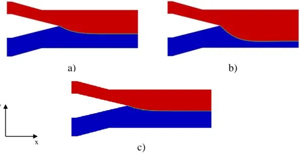
After performing a test simulation in order to optimize some parameters required by the interFoam solver, by checking the results obtained it was observed that after three seconds the flow reached steady stated conditions. For that reason, all the simulations were performed for a maximum time of 3 𝑠 and the time step used (including the test simulation) was equal to 1 × 10⁻⁶ 𝑠. Figure 16 shows the materials distribution when the equilibrium is reached for the three case studies, with the more refined mesh created using
cfMesh (in the Appendix A are the results to the corresponding meshes created using blockMesh).
Analysing Figure 16, it can be observed that the less viscous layer (P3 blend) is supressed by the one with the higher viscosity (P2 blend) in all the tested cases. In Case 2, due to the difference between the velocity imposed to the P2 blend and the velocity imposed to the P3 blend, the suppression of the P3 mixture is more severe than in the other two cases, while in these two cases the suppression of the less viscous layer is more or less the same. This domain distribution is a direct outcome of the viscosity differences, since the flow domains arranged in order to have the same axial pressure gradient. Since P2 has a higher viscosity the layer must be thicker to reduce its velocity and, thus the axial pressure gradient, and the opposite occurs for P3. In this way the axial pressure gradient is balanced in both domains.
Showing the location of the domain containing 50% of the both phases, it is possible to obtain the coordinates of the interface points and thus compare those with the
Figure 16 - Steady state flow for 2D coextrusion case study, for the more refined mesh created using cfMesh in: a) Case 1; b) Case 2; c) Case 3.
a)
b)
y
x
interface points presented in the comparison paper (Hannachi & Mitsoulis, 1993). Attending to the fact that the paper only possesses a graphical representation of the interface points, it was necessary to obtain the coordinates of these points. Those calculations were made by the open source software Engauge Digitizer, where defining the coordinate system, the software generates the coordinates of a set of points belonging to the interface between the two materials. It is important to mention that the figures used from the paper are old and with poor resolution, which may lead to some inaccuracy of the results. Figures 17, 18 and 19 illustrate the graphics comparing the localization of the interface obtained with the OpenFOAM computational library with the results presented in the paper. -0,004 -0,0035 -0,003 -0,0025 -0,002 -0,0015 -0,001 -0,0005 0 0 0,005 0,01 0,015 0,02 0,025 0,03 y (m) x (m)
Interface development in Case 2 with mesh
created using cfMesh
M1 M2 M3 M4 Benchmark
Figure 18 - Interface coordinates for Case 2 (mesh created using cfMesh). Figure 17 - Interface coordinates for Case 1 (mesh created using cfMesh).
-0,002 -0,0015 -0,001 -0,0005 0 0 0,005 0,01 0,015 0,02 0,025 0,03 y (m) x (m)
Interface development in Case 1 with mesh
created using cfMesh
M1 M2 M3 M4 Benchmark
From the previous figures it is possible to observe that in Case 1 and in Case 2, as the mesh is refined, the interface position tends to converge to the solution presented in the paper (benchmark). In Case 3, the results obtained are converging to a solution that is not the solution presented in the paper. This may be explained by an error in the mass flow rates provided in the paper.
Regarding the results obtained with the meshes created by the blockMesh utility, they are more or less the same than those obtained for the meshes created with cfMesh, not having significant differences between them, as can be seen comparing Figure 17 with Figure 20 (in the Appendix B are the graphics for the other cases).
Figure 19 - Interface coordinates for Case 3 (mesh created using cfMesh).
-0,002 -0,0015 -0,001 -0,0005 0 0 0,005 0,01 0,015 0,02 0,025 0,03 y (m) x (m)
Interface development in Case 1 with mesh
created using blockMesh
M1 M2 M3 M4 Benchmark
Figure 20 - Interface coordinates for Case 1 (mesh created using blockMesh).
-0,003 -0,0025 -0,002 -0,0015 -0,001 -0,0005 0 0 0,005 0,01 0,015 0,02 0,025 0,03 y (m) x (m)
Interface development in Case 3 with mesh
created using cfMesh
M1 M2 M3 M4 Benchmark