DEPARTAMENTO DE ECONOMIA
PROGRAMA DE PÓS-GRADUAÇÃO EM ECONOMIA
Optimal Legislative Funding
Financiamento Ótimo do Legislativo
Beatriz Silva Garcia
Orientador: Prof. Dr. David Turchick
Prof. Dr. Adalberto Américo Fischmann
Diretor da Faculdade de Economia, Administração e Contabilidade
Prof. Dr. Hélio Nogueira da Cruz
Chefe do Departamento de Economia
Prof. Dr. Márcio Issao Nakane
Optimal Legislative Funding
Financiamento Ótimo do Legislativo
Dissertação apresentada ao Departamento de Economia da Faculdade de Economia, Admi-nistração e Contabilidade da Universidade de São Paulo como requisito parcial para a obtenção do título de Mestre em Ciências.
Orientador: Prof. Dr. David Turchick
Versão Corrigida
São Paulo - Brasil
FICHA CATALOGRÁFICA
Elaborada pela Seção de Processamento Técnico do SBD/FEA/USP
Garcia, Beatriz Silva
Optimal legislative funding / Beatriz Silva Garcia. – São Paulo, 2016. 83 p.
Dissertação (Mestrado) – Universidade de São Paulo, 2016. Orientador: David Daniel Turchick Rubin.
1. Formação de governo 2. Barganha legislativa 3. Financiamento do legislativo 4. Rent-seeking 5. Votação estratégica I. Universidade de São Paulo. Faculdade de Economia, Administração e Contabilidade. II. Título.
Agradeço imensamente aos meus pais, irmãs, avós e sobrinhos, por terem me
apoiado e incentivado incondicionalmente durante toda a minha trajetória. Estiveram ao
meu lado e deram todo o suporte necessário durante os momentos de conquistas e desaĄos
que passei ao longo dessa fase.
Ao meu orientador, Prof. David Turchick, que se manteve à disposição e presente
em todas as etapas desse trabalho de forma tão solícita e sempre me incentivou a trilhar
uma trajetória dedicada à pesquisa. Ao Prof. Marcos Nakaguma, pelos conselhos essenciais
para o desenvolvimento desse projeto.
Agradeço imensamente também aos amigos que Ąz e mantive durante toda esse
período e que direta ou indiretamente me ajudaram, apoiaram e incentivaram para a
conclusão dessa etapa. Estiveram presentes dividindo os momentos de conquistas e de
desaĄos, tornando essa etapa uma grande experiência de crescimento pessoal e acadêmico.
Por Ąm, agradeço ao apoio Ąnanceiro concedido pelo Conselho Nacional de
Propõe-se um modelo teórico para estudar a formação de governo por um corpo legislativo,
composto por partidos eleitos em representação proporcional. Uma vez que a conĄguração
do Legislativo é deĄnida, os partidos eleitos devem formar um governo, escolher uma
política de governo e uma distribuição de recursos e benefícios legislativos entre os partidos
presentes na casa através de um jogo de barganha. Uma massa de eleitores é assumida
capaz de votar estrategicamente. Nosso objetivo é estudar como uma limitação nos recursos
disponíveis entre os legisladores pode afetar o comportamento dos agentes envolvidos no
sistema, tanto eleitores quanto legisladores. Mostra-se que uma queda da distância relativa
entre as ideologias aumenta o bem-estar social e diminui a quantia necessária de recursos
que mantem o acordo legislativo ótimo. Ademais, há um limite superior para essa quantia
quando a distância ideológica aumenta.
Palavras-chaves: formação de governo, barganha legislativa, Ąnanciamento do legislativo,
We propose a model to study government formation by a legislative body composed by
parties elected with a proportional representation rule. Once the legislative conĄguration
is determined, the elected parties must form a government, choose a government policy
and a distribution of legislative resources and beneĄts among the elected parties through
a bargaining game. A mass of voters is assumed capable of voting strategically. Our goal
is to study how a limitation on the available resources among legislators may afect the
behavior of the agents involved in this system, both voters and legislators. We show that
a decrease in the relative distance between ideologies increases the social welfare and
decreases the necessary amount of resources to keep the optimal agreement. Moreover,
there is an upper limit to this amount when the ideological distance increases.
Keywords: government formation, legislative bargaining, legislative funding, rent-seeking,
1 Introduction . . . 13
2 The model . . . 17
3 Legislative Equilibrium . . . 21
4 Electoral Equilibrium . . . 33
5 Social Welfare . . . 41
6 Conclusion . . . 45
References . . . 47
1 Introduction
Life in society requires articulation among its members to deĄne rules and policies.
In this organization, the government can be seen as the highest body in a decision hierarchy.
The study of government formation is then essential to understand how policies are deĄned.
In a dictatorial system, where an individual or just an ideologically homogeneous group is
the top of the decision chain, an explicit articulation is not necessary, since everybody is
subject to the choices of the homogeneous group in power.
In such a system, ideologies of individuals are completely ignored for policy
deter-mination, therefore, unless the dictator is a representative agent of society or a benevolent
central planner, social welfare will not be at its optimum.
In a democratic system, however, the deĄnition of an election rule in which members
of society choose the participants in the highest decision body is required. When this body
is composed of a legislative body, the lowest heterogeneity in preferences of the participants
makes coalition formation a necessary and fundamental factor of system stability. In the
parliamentary, the government is deĄned by the coalition that has the support of the
majority of parties in the legislature.
The coalition formation process is carried out through a bargaining game in which
the parties negotiate and make agreements on the conditions necessary for a majority
group to support a common government policy.
The parties and votersŠ behavior in a representative system is the subject of a
wide range of studies. However, the impact of restricting the resources that parties use
for political bargaining is not directly considered in those studies. This work proposes a
theoretical investigation on the impact of this restriction, since the resourcesŠ magnitude
is an important element of the coalition formation that may afect the behavior of both
agents in the electoral process, voters and parties.
Diferent studies analyze the formation of coalitions and factors possibly relevant
Laver (1998), which summarizes diferences in approach and methodology.
Laver (1998) considers basically two hypotheses about the motivations of parties:
the oice-seeking and the policy-seeking assumptions. In the Ąrst case, parties base their
decisions on the desire to get into oice and derive some beneĄt from taking part in the
government. In the second case, the parties are concerned with the government policies and
their main interest is getting into oice in order to inĆuence these policies. It is common
to consider a mix of these two motivations for a better representation of reality.
At the bargaining process, each party has the chance of making a proposal to other
parties by suggesting a government policy and a portfolio distribution. If it has the support
of the majority of the house, this coalition succeeds and the government is formed. This
portfolio is a Ąxed amount of resources and beneĄts that can be distributed among parties
in the legislature. We assume parties are interested both in supporting a government policy
ideologically close to its ideal policy and also in receiving as many beneĄts as possible.
Bandyopadhyay & Chatterjee (2006) survey several speciĄcations for this bargaining
process, and Martin & Stevenson (2001) test several assumptions usually used in theoretical
approaches. Some of their main results are that in fact both policy seeking and oice
seeking have a signiĄcant role for government formation indeed and that the government
coalition usually includes the largest legislative party
However, it is important to stress that voters have a great role in democratic
parliamentary systems, since they are responsible for determining the composition of the
legislature. Despite of the fact that the individuals do not take part into the government,
they also have preferences on the government policy. Therefore, voters will be concerned
with the government policy that is supported by the legislative body.
Assuming perfect information among agents, i.e. everyone is fully aware of the
preferences of all involved, voters are able to anticipate the behavior of parties in the
legislature, and they will thus vote in such a way that the political government arising
we call strategic voting. When it is not possible, voters show sincere voting, in which they
vote for the party that represents their ideology, with no need to consider the agreements
that the parties can reach in the legislature.
This relation between votersŠ behavior and coalition formation in the legislature has
been the concern of several empirical and theoretical studies. For instance, Debus & Müller
(2013) show how votersŠ preferences could also impact the coalition formation and the
government outcomes. Herrmann (2014) presents empirical evidence on strategical voting.
He shows how election polls can inĆuence votersŠ decisions by changing their expectations
about coalition formation.
To the same end, Armstrong & Duch (2010) analyze the historical patterns in
coalition formation as an indicative of the possibility of strategic behavior in votersŠ
decisions. Hobolt & Karp (2010) also study the conditions that lead to voters to adopt
strategic behaviors under elections on plurality and proportional systems. Duch, May &
Armstrong (2010) empirically show that this behavior is common in systems with coalition
government formation.
Once determined how voters and parties behave, we are able to describe the system
equilibrium from the interaction of agents in each stage: electoral and legislative.
The research developed by Austen-Smith & Banks (1988) proposes a general model
that includes three stages of government formation. In the Ąrst stage (pre-election), parties
announce the ideology they seek to defend at the legislature. Then, voters decide for which
party to vote. The shares of votes obtained by each party determines the number of seats
they will occupy at the legislature. In the last stage, the elected parties participate in a
bargaining game to form a government and decide on a government policy and a division
of the legislative resources.
Analyzing the whole system, we can identify factors and incentives that lead to
objective and veriĄable behavior of agents. The available legislative resources have an
with diferent ideology to join them in a voting on policy. Thus, it is intuitive that the
magnitude of this legislative resources has an important role on the coalitions formations.
A larger amount can increase the advantage of the party that decides how it will be divided.
If a larger amount we suppose that it will be able to convince a bigger set of parties, and
if the resources decrease, its set of possibilities may reduce. We can thus predict changes
in the behavior of parties in the coalition formation and therefore in the voting behavior
in the elections process.
In view of this, we intend to study how limitations on legislative resources, which
would impact directly the representativesŠ payofs, thus changing the pattern of their
behavior could be welfare optimizing.
Our main goal is to identify the impact of restricting the bargaining power of the
parties in the legislature on government outcomes and social welfare. In fact, we assume
within the legislative body structure the formation of coalitions and party connections
through the exchange of beneĄts and resources. Hence, a decrease in the size of these
beneĄts may act as a restrainer on partiesŠ bargaining power.
Since the size of this portfolio can inĆuence the outcome of the bargaining game,
we shaw employ a model similar to the one proposed by Austen-Smith & Banks (1988) in
order to analyze how the resource constraint impacts government outcome.
In the following chapter, we will describe our model and hypotheses. Chapter 3 and
4 are devoted to the analysis of the efects on social welfare and the optimum magnitude
of legislative resources.Chapter 5 concludes, while the proofs to the aforementioned
2 The model
We propose a model to study a government formed by a legislative body, in which
the council is composed by parties elected with a closed-list proportional representation
rule. Each party announces a list of candidates to take part in the legislature and the
seats are allocated according to the proportion of votes obtained by each party. Once
the legislative conĄguration is deĄned, they will choose the government policy and the
distribution of the portfolio of legislative resources among the elected parties through a
bargaining game.
In fact, we observed in the legislative policy structure the formation of coalitions
and party connections made through exchange of beneĄts and resources between the
parties in order to form up a majority group. Since the size of this portfolio can inĆuence
the outcomes of this bargaining game, the central aim of this model is to analyze how the
resource constraint can impact the government policy.
An expected result would be that unlimited resources could ensure the formation
of coalitions among ideologically distant parties, leading to a distant equilibrium of
government policy that would be socially optimal. In return, the presence of resources that
allow partisan negotiations bargaining is necessary for the legislative between consensus
to preserve the governability. This trade-of arises the need of deĄning the optimal size of
these resources available in the house in such a way that maximizes social welfare.
To this end, we adopt a simpliĄcation of the three periods model proposed by
Austen-Smith & Banks (1988). Besides those mentioned above, they also propose a Ąrst
period when each party chooses its policy position, so they can maximize its vote share
at the elections. In our model, we consider that party ideologies are exogenously deĄned.
Each party is interested in representing one group of voters.
Let Ω =¶Ð, Ñ, Ò♢ be a discrete space of ideologies. The ideological distribution of voters is given by the vector à= ¶àÐ, àÑ, àÒ♢. By a correspondence between the ideological
policy, (�Ð, �Ñ, �Ò).
Unlike the model of Austen-Smith & Banks (1988), the parties electoral strategy
and how they choose which ideological position they will defend is not our concern. We
only assume that there will be a party representing each group of voters. Therefore, we
deĄne three parties Φ =¶�, �, �♢ with the following ideal policy respectively:
��= ���¶�Ð, �Ñ, �Ò♢
�� = ���¶�Ð, �Ñ, �Ò♢
��= ���¶�Ð, �Ñ, �Ò♢
These parties are elected to compose the legislative body by a closed-list proportional
representation rule. Each party announces a list of candidates in the pre-electoral period
and voters choose a party to vote for. Then, the seats of the legislature are allocated
among the parties, according to the proportion of votes obtained by each one, and the
candidates that get the seats are deĄned by the partyŠs list.
Voters can show two types of behavior: sincere voting and strategic voting. The
Ąrst one consists of choosing the party that represents their ideal policy, regardless of the
other votersŠ choice. Alternatively, voters may be more concerned about the government
policy arising from the legislative process. Therefore, they decide their vote based on the
expected outcome of the bargaining game and not just the policy position of the party.
If voters are aware that their vote can inĆuence the government policy and are able to
anticipate the equilibrium of the legislative stage, they can attempt to vote strategically
rather than sincerely.
We assume that only voters with the ideal policy �� vote strategically. Thus,
voters with extreme ideologies, represented by parties � and�, will necessarily vote for the party that represents them, i.e. will vote sincerely. We also assume that the strategic
group of voters behaves in a coordinated way. In other words, they can organize and deĄne
the portion of its members that will vote for each party, ensuring that the legislature
Following the election, the participation of parties in the house is represented by
the vectorw= (��, ��, ��). This distribution of seats is exactly equal to the proportion
of votes obtained, i.e. there is no requirement of a minimum number of votes for the party
to be elected.
Once the conĄguration of seats in the house is deĄned, the elected parties should
choose the government policy, � ∈ �, by a simple majority poll. It is also up to the legislature the decision of how the funds and beneĄts of the house, represented by the
exogenous variable�, should be divided among the elected parties Ű that is, to choose a pointg from Δ(�) = ¶(��, ��, ��)∈R3 :�� ⊙0,∀�∈Φ, ︁
�∈Φ��
=�♢.
When a party has numerical majority in the house, it has enough power to win
the poll alone, so it can deĄne government policy according to its ideal and hold all the
resources of the house. Otherwise, a bargaining game between the parties begins and there
is the formation of a minimum coalition that supports an agreed policy. As we shall see in
the next chapter, in equilibrium every party gets a set in the house. Since we have three
parties, the bargaining game holds in up to three periods.
In the Ąrst period,� = 1, the largest party makes a proposal for a winning coalition
�⊖Φ Ű that is, one such that �� >1/2, where�� =︁�∈���. Since there will be three
parties in the house, unless the largest party has more than 50% of the seats, any subset
of Φ of size 2 will be a winning coalition. The proposal consists of a government policy�1
and a distribution of the resourcesg1= (�1�, �1�, �1�). The party invited for the coalition
accepts or rejects the proposal. If it is accepted, the government is formed and the game
ends, otherwise, the bargaining continues to the next period, in which the second largest
party tries to form a winning coalition.
If it is not successful in this task, the smallest party gets to make the ofers at�= 3. However, if no agreement is met in any of the periods, since the parties did not reach any
consensus, no policy will be established and no beneĄts will be distributed among them.
In the case of a tie between any parties at the elections, the order in which they
will make their coalition proposals will be deĄned by a coin toss before the beginning of
the bargaining game (� = 0).
As such, once party � is elected, its preferences are represented by the utility function:
��(�, ��) =
︁ ︁ ︁ ︁ ︁ ︁ ︁ ︁
︁ ︁ ︁ ︁ ︁ ︁ ︁
��⊗(�⊗��)2 if � is elected and a government is formed
0 if � is elected and no government is formed
⊗� if � is not elected
(2.1)
where �is a constant such that �⊙(��⊗��)2.
For the votersŠ preferences, we assume that their utility depends on lump sum
tax, paid by every voter and is intended for the legislature resources, and the idealogical
distance between the government policy and their ideal policy. Thus, the utility for voter�
is��(�) =⊗�⊗(�⊗��)2. However, if the legislative body cannot achieve an agreement
through this bargaining game, there is no consensus and no policy will be adopted. In this
case, we deĄne that all voters will obtain the worst possible utility:�� =⊗�⊗�.
Thereby, the model proposed is based on a sequential game with two stages:
elections are held for the composition of the house (�= 0), and then elected parties decide the government policy from a bargaining game and the government is formed (�= 1,2,3). Since we assume a game with perfect information among the agents, i.e. the action of
each period can be anticipated, the game can be solved by backward induction. First, we
analyze the legislative stage and Ąnd the equilibrium policy for a given distribution of
3 Legislative Equilibrium
As mentioned above, once the legislative body is elected, the government policy
should be chosen by the house with a majority poll and the outcomes depend on the
proportion of each party in the house, w = (��, ��, ��). If there is a party with the
numerical majority, it can support its own ideal policy and hold all the house resources.
Otherwise a bargaining game begins, so that a winning coalition is formed in order to
elect a government policy.
In the following analysis, we describe in detail the bargaining process in the case
in which the parties have distinct shares in the legislature. We assume that, in case of a
tie between the parties in the election, the order by which they make the proposals of
coalitions is deĄned tossing a coin before the bargaining game starts. The results of these
cases are also described in the analysis presented below.
When a party is deciding which proposal it will make, it is necessary to ensure that
the other party invited for the coalition is willing to accept it. Thus, the proposal must
give the other party at least the same utility that it would obtain if it rejects the proposal.
At� = 3, the outside option of accepting a proposal is a situation with no agreement, in which every party obtains zero utility. However, in the other periods, the opportunity cost
of accepting a proposal is the utility obtained with the agreement of the following period.
This reservation utility for party � at period �,���, can be expressed as:
�3�=0
�2�=��(�3,g3) = �3�⊗(�3⊗��)2
�1�=��(�2,g2) = �2�⊗(�2⊗��)2
where �� and ��� are the government policy and the beneĄts obtained by party � through
the proposal agreed upon at period �.
We assume a game with perfect information, so that parties are able to anticipate
party possesses the absolute majority of the seats, a singleton winning coalition emerges.
Otherwise, an agreement between two parties is suicient to form a winning coalition �
with�� >1/2. To decide which will be the optimum proposal, we have to compare the
utility obtained in every possible coalition. If party � makes the proposal at period �, it will choose the coalition with the agreement that gives itself the greatest possible utility.
Suppose that party� proposes a coalition with party� at period�. The optimum proposal
must maximize the following problem:
max
g,� ��⊗(�⊗��)
2
s.t. ��⊗(�⊗��)2 ⊙��� (3.1)
��⊗(�⊗��)2 ⊙��� (3.2)
��+�� +�� =� (3.3)
��, ��, ��⊙0 (3.4)
Note that (3.1) makes the proposal worthwhile for party �, otherwise it will prefer the agreement of the following period; (3.2) ensures the minimum utility that makes party
�, invited to the coalition, willing to accept the proposal (we assume that when a party is indiferent between accepting or not a proposal, it chooses to take on the agreement);
(3.3) and (3.4) are the requirements of the distribution of beneĄts among the parties.
Additionally, for ��� ⊙ 0, restriction 3.2 will hold with equality. Otherwise, if
�� ⊗(�⊗��)2 > ��� ⊙ 0, we would have �� > ��� + (�⊗��)2 ⊙ 0. Thus, for any value
of �, �Šs utility could be increased by decreasing �� until the constraint is satisĄed with
equality. Therefore, all problems below are simpliĄed using the equality on this restriction,
if ��� ⊙0.
Let �= (��,gt, ��) be the optimal proposal for period �, where �� is the optimum
government policy at �; gt is the optimum distribution at �; and �� is the minimum
coalition formed at�. As we assume perfect information and the bargaining game is solved by backward induction, the legislative equilibrium will be a subgame perfect equilibrium.
government policy of the equilibrium at the legislative stage, we can mention:
1. When party� is the Ąrst one to make a coalition proposal, it will be able to form a coalition with the smallest party that supports �Šs ideal policy as the government
policy even with party � holding all the resources �. The magnitude of � will deĄne the conditions in which this agreement will be possible. If it is not suiciently
large, the equilibrium will be a no-deal situation on the house.
2. When party� is the second one to make a coalition proposal, the party with the most seats in the legislature will choose to make a coalition with the smallest party,
regardless of the ideological distances. A decrease in the magnitude of �can lead to a government policy closer to the ideal policy of the largest party. It can beneĄt this
group, but the impact on social welfare is ambiguous.
3. When party� is the last one to make a proposal, the decrease of �Šs magnitude can
sometimes improve the utility of the majority of voters by leading to a government
policy closer to their ideal policy. However, this impact of�on the government policy depends on the ideological distance setting and will be analyzed afer we include an
other important element of the model: votersŠ behavior.
We shall now describe the equilibrium achieved at each period for all possible
legislative conĄgurations, which summarizes the equilibrium for each scenario. Followed by
Proposition 1, detailed proofs of each step can be found in the Mathematical Appendix.
First, we analyze the case in which party� holds the greatest participation in the legislature, for instancewM>wR >wL.1 The party with the lowest weight in the house,
�, makes the proposal at �= 3. Since all parties have the same opportunity cost at �= 3, party� will choose the closest party to form a coalition, �. The optimum proposal in
1
this case will be the solution of the problem:
max
g,� ��⊗(�⊗��)
2
s.t. ��⊗(�⊗��)2 ⊙0
�� ⊗(�⊗��)2 = 0
��+�� =�
��, �� ⊙0
In order to simplify the notation, for any �, ℎ ∈ Φ, let ��ℎ be the mid-distance
policy between�� and �ℎ: ��ℎ =(�j+�h)/2.
If�⊙2(�� ⊗�� �)2, then the solution for the problem above will be:
�∗
3 =�� �
�3� =�⊗(�� ⊗�� �)2
�3� = (�� ⊗�� �)2
�3� = 0
�3 =¶�, �♢
This solution is the same as in Austen-Smith & Banks (1988), since they consider that
the beneĄt � is suiciently large so that any coalition can be formed. However, if� <
2(�� ⊗�� �)2, no agreement will be met.
Actually, this reasoning holds for every conĄguration in the legislature. Since the
problem at� = 3 is similar regardless of which party is the smallest, whoever is making the proposal will choose the ideologically closest party to form the coalition and will propose
a similar government policy and beneĄt distribution as shown above.2
Lemma 1. For any given distribution of parties in the legislature, let � be the party that makes the proposal at � = 3 and ♣�� ⊗�ℎ♣ < ♣�� ⊗��♣. If � ⊙ 2(�� ⊗��ℎ)2, then the
2
optimal proposal at this period will be:
Γ3 = ︁ ︁ ︁ ︁ ︁ ︁ ︁ ︁ ︁ ︁ ︁ ︁ ︁ ︁ ︁ ︁ ︁ ︁ ︁ ︁ ︁ ︁ ︁ ︁ ︁ ︁ ︁ ︁ ︁
�3 =��ℎ
�3� =�⊗(��⊗��ℎ)2
�3ℎ = (�� ⊗��ℎ)2
�3 =¶�, ℎ♢
If � <2(�� ⊗��ℎ)2, then no agreement will be met.
In order to simplify our analysis, we make three assumptions. If a party is indiferent
between making a proposal to one or anouther party, it will choose the ideologically closest
one. If it is ideologically equidistant to the two other parties, it will choose the party
with the lowest participation in the house. In the case of indiference between making an
agreement or not, we also assume that parties will always prefer to do so.
Let�� ⊕��⊗�� and��⊕��⊗��. Still with the �� > ��> �� case in mind,
the relevant threshold for� becomes 2(��⊗�� �)2 = 2 (�L/2)2 =(�L)2/2.
The opportunity costs of each party at the previous period,� = 2, are:
If �⊙ (��)
2
2 , �2� =��(�� �,0) =
⊗(2��+��)2
4
�2� =��
︁
�� �,(�� ⊗�� �)2
⎡
= 0
�2� =��
︁
�� �, �⊗(�� ⊗�� �)2
⎡
=�⊗ (��)
2
2
If � < (��)
2
2 , �2� =�2� =�2�= 0
Since party � has the closest ideology to party � and it also has the lowest opportunity cost, it will be optimal for party� to propose a coalition to party� at� = 2.3
The optimal proposal will be a function of the ideological distances between the parties,��
and��, and the size of the legislative resources,�. As � increases, the government policy
proposed for the coalition will get closer to the ideal policy of party �. The ideological distances will determine the size of� necessary to support each policy.
3
At� = 1, party � makes a proposal anticipating all the following periods. Since the outside option of its proposal is an agreement with the coalition�2 =¶�, �♢and a
government policy �2 ∈[��, ��], we have �1� =��(�2,0) = ⊗(�2 ⊗��)2, whence party
� can make a proposal to party � with its own ideal policy as the government policy, since��(��, �1�)⊙ ⊗(�� ⊗��)2 ⊙ ⊗(�2⊗��)2, ∀�2 ∈[��, ��]. Thus, it is possible for
� to ensure a higher utility to party �and to increase its own utility, even by holding all the resource beneĄts�.
However, there is a lower bound for the size of�that ensures na agreement in each period of the bargaining game. If such a minimum is not met, that rationale above would
be invalid, since the opportunity costs would be ��� = 0, ∀� ∈ 1,2,3, � ∈ Φ. Thus, the
maximization problem faced at each period would be similar to that described in Lemma
1.4
Now suppose that party � is the second largest party in terms of legislative participation, for instancewR >wM >wL.5 At� = 3, the optimal proposal is determined
by party�as set out in Lemma 1. Thus, for�⊙(�L)2/
2the optimal coalition is�3 = ¶�, �♢
and the government policy is�3 =�� �. Otherwise, no agreement is met.
At �= 2, for �⊙1/2(��)2, party � should choose between a coalition with party
� or �. In the appendix, we show that an agreement with party� would provide a higher utility for party �, regardless of the ideological distances between parties. Since the
outside option for its proposal is the government policy�3 =�� � with a coalition between
� and �, party � can propose to party � an agreement with its own ideal political position,��, as the government policy and thus can also give a higher utility to party �,
without sharing the legislative resources,�.
However, if� <1/2(��)2 and party� is closer to party�, �
� < ��, the outside
option for this case is a no agreement situation where all parties obtain zero utility.
Therefore, for � suiciently large (⊙(�R)2/
2), it is possible to make a coalition with the
4
Details can be found in the mathematical appendix.
5
closest party �, as proved in Lemma 1. Otherwise, a no deal situation is even better for the proponent.
At � = 1, when party � makes the proposal, if it chooses a coalition with party
�, the only feasible agreement is the same one made at � = 2. However, if it choses a coalition with party�, it is possible for party� to obtain a greater utility. For�⊙(�L)2/
2,
the optimum proposal is �∗ = �
� and ��∗ = �, regardless of the ideological distances.
For (�L)2/
2 > � ⊙ (�R)2/2 and �� > ��, the optimum proposal is �∗ = ��� and ��∗ = �.
Otherwise, it will prefer a no deal situation where everyone obtains zero utility. Therefore,
a lower amount of resources �can lead to a government policy closer to the ideal policy of the major party.
This result indicates the importance of analyzing the impact of� on social welfare, which we leave to chapter 5. On one hand, a reduction of � increases the utility of all voters, since this resource comes from a lump-sum tax paid by all of them. On the other
hand, note that as it leads to a government policy closer to the ideal policy of the group
with the greatest presence in the legislature. At least one other group (but possibly both,
which may account for the majority of voters) becomes worse of.
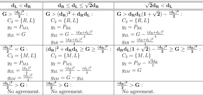
Finally, suppose that party � holds the lowest participation in the legislature, for instancewR >wL >wM.6 At � = 3, party� will make a coalition with the closest
party, as prescribed by Lemma 1. At� = 2, if � is suiciently large to compensate for
the ideological distance, party � will prefer a coalition with the party with the lowest opportunity cost at that period, �. However, as the value of � decreases, it may become better for party �to choose the closest party, �, even with its higher opportunity cost. The proposal will also difer by value of � and the ideological distances setting. The optimum solutions for this period are summarized in the following table:
6
Table 1 Ű Optimum settlements at period� = 2 (�� > ��> ��)
dL <dR dR ⊘dL ⊘√2dR √2dR <dL G> (dL)2
2 : G>(dR)
2+dRdL : G>dRdL(1+√2)⊗(dL)2
2 :
�2 =¶�, �♢ �2 =¶�, �♢ �2 =¶�, �♢
�2 =�� � �2 =��� �2 =���
�2�=� �2�=�⊗ (�R+�L)
2
4 �2� =�⊗
(�R+�L)2
4
�2�= (�R+�L)
2
4 �2� =
(�R+�L)2
4 (dL)2
2 =G: (dR)
2+dRdL
⊙G⊙ (dR)2
2 : dRdL(1+
√
2)⊗ (dL)2
2 ⊙G⊙
(dR)2
2 :
�2 =¶�, �♢ �2 =¶�, �♢ �2 =¶�, �♢
�2 =�� � �2 =�� � �2 =�� ⊗
√
2�R
2
�2�= (�L)
2
4 �2�=
(�R)2
2 ⊗
(�L)2
4 �2� =�
�2� = (�L)
2
4 �2� =�⊗�2�
(dL)2
2 >G:
(dR)2
2 >G:
(dR)2
2 >G:
No agreement. No agreement. No agreement.
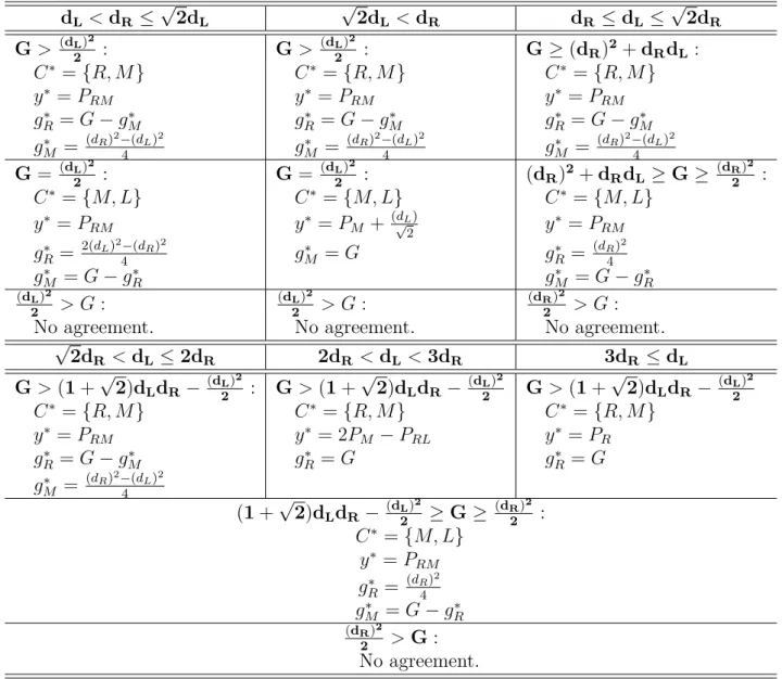
At � = 1, since party � will have the lowest opportunity cost and it is also the closest party to� in terms of ideological distance, there will not be a trade-of between
establishing an agreement with party �or �. Therefore, the optimum coalition will be between parties� and �, regardless of the ideological distances setting and the value of
Table 2 Ű Optimum settlements at period� = 1 (�� > ��> ��)
dL <dR ⊘√2dL √2dL <dR dR ⊘dL⊘√2dR G> (dL)2
2 : G>
(dL)2
2 : G⊙(dR)
2+dRdL:
�∗ =¶�, �♢ �∗ =¶�, �♢ �∗ =¶�, �♢ �∗ =��� �∗ =��� �∗ =��� �∗ � =�⊗�∗� ��∗ =�⊗��∗ ��∗ =�⊗��∗ �∗ � =
(�R)2−(�L)2
4 ��∗ =
(�R)2−(�L)2
4 ��∗ =
(�R)2−(�L)2
4
G= (dL)2
2 : G=
(dL)2
2 : (dR)
2+dRdL ⊙G⊙ (dR)2
2 :
�∗ =¶�, �♢ �∗ =¶�, �♢ �∗ =¶�, �♢ �∗ =�
�� �∗ =�� + (√�L2) �∗ =���
�∗
� =
2(�L)2−(�R)2
4 ��∗ =� ��∗ =
(�R)2
4
�∗
� =�⊗��∗ ��∗ =�⊗��∗
(dL)2
2 > � :
(dL)2
2 > �:
(dR)2
2 > �:
No agreement. No agreement. No agreement.
√
2dR <dL⊘2dR 2dR<dL <3dR 3dR ⊘dL G>(1+√2)dLdR⊗ (dL)
2
2 : G>(1+
√
2)dLdR⊗ (dL) 2
2 G>(1+
√
2)dLdR⊗ (dL) 2
2
�∗ =¶�, �♢ �∗ =¶�, �♢ �∗ =¶�, �♢ �∗ =�
�� �∗ = 2�� ⊗��� �∗ =��
�∗
� =�⊗�∗� ��∗ =� ��∗ =�
�∗
� =
(�R)2−(�L)2
4
(1+√2)dLdR⊗ (dL)2
2 ⊙G⊙
(dR)2
2 : �∗ =¶�, �♢ �∗ =� �� �∗ �=
(�R)2
4
�∗
� =�⊗��∗
(dR)2
2 >G:
No agreement.
Again, we can observe from this equilibrium an efect of the magnitude of �on the government policy. Depending on the ideological distance setting, the decrease of� can sometimes beneĄt the majority of voters and sometimes distance the government policy
from their ideal point. A detailed analysis is presented in chapter 5 after including votersŠ
behavior in the elections.
The equilibrium for any legislature conĄguration is described by the following
theorem.
1. If party � has the majority in the house, �∗ =�
� and �∗�=�, regardless of the size
of �;
2. If no party has the majority, we have the following possible cases:
a) Party M proposes at t=1: If � ⊙ (�i)2/
2, where �� = min¶��, ��♢, the
equilibrium will be �∗ = ¶�, �♢, where �
� = min¶��, ��♢, �∗ = �� and
�∗
� =�. Otherwise, no agreement is met.
b) Party M proposes at t=2: The optimum coalition will be �∗ = ¶�, �♢
and the best proposal will depend on the value of � and the ideological distance
setting:
• If �⊙(�j)2/
2, �∗ =�� and ��∗ =�.
• If (�j)2
/2> �⊙(�k)2/2, �∗ =(�M+�k)/2 and �∗� =�.
Otherwise, no agreement is met.
c) Party M proposes at t=3: The optimum coalition will be �∗ = ¶�, �♢,
where �� =���¶��, ��♢ and the best proposal will depend on the value of �
and the ideological distance setting:
• For �ℎ ⊙3��:
– If� > (1 +√2)�ℎ��⊗(�h)2/2, the optimum will be�∗ = �� and ��∗ =�.
– If (1 +√2)�ℎ��⊗(�h)2/2⊙�⊙(�k)2/2, the optimum will be �∗ =���,
�∗
� =(�k)2/4 and �∗� =�⊗�∗�.
• For 2��< �ℎ <3��:
– If� > (1 +√2)�ℎ��⊗(�h)2/2, the optimum will be�∗ = 2��⊗��ℎ and
�∗
� =�.
– If (1 +√2)�ℎ��⊗(�h)2/2⊙�⊙(�k)2/2, the optimum will be �∗ =���,
�∗
� =(�k)2/4 and �∗� =�⊗�∗�.
• For √2�� < �ℎ ⊘2��:
– If� > (1+√2)�ℎ��⊗(�h)2/2, the optimum will be�∗ =���,�∗�= �⊗��∗
and �∗
– If (1 +√2)�ℎ��⊗(�h)2/2⊙�⊙(�k)2/2, the optimum will be �∗ =���,
�∗
� =(�k)2/4 and �∗� =�⊗�∗�.
• For ��⊘�ℎ ⊘√2��:
– If � > (��)2+���ℎ, the optimum will be �∗ =���, ��∗ =�⊗�∗� and
�∗
� =(�k)2/4⊗(�h)2/4.
– If(��)2+���ℎ ⊙�⊙(�k)2/2, the optimum will be�∗ = ���,�∗� =(�k)2/4
and �∗
� =�⊗��∗.
• For √2�ℎ < �� < �ℎ:
– If � > (�h)2/
2, the optimum will be �∗ = ���, �∗� = � ⊗��∗ and
�∗
� =(�k)
2
/4⊗(�h)2/4.
– If �=(�h)2
/2, the optimum will be �� +�h/√2 and ��∗ =�.
• For �ℎ < ��⊘
√ 2�ℎ:
– If � > (�h)2
/2, the optimum will be �∗ = ���, �∗� = � ⊗��∗ and
�∗
� =(�k)2/4⊗(�h)2/4.
– If �=(�h)2/
2, the optimum will be�∗ =���, ��∗ =(�h)2/2⊗(�k)2/4 and
�∗
� =�⊗��∗.
Otherwise, no agreement is met.
Note that the intervals of � above are deĄned by quadratic functions of the ideological distances, and that the government policy� is deĄned by a linear function of
�� and the ideological distances. Thus, considering the following transformations, we can
reduce the number of variables in the model, in order to make the graphical display of
such relations easier. We consider from now on the following variables:
• � =�L/�R;
• � =�/(�R)2;
• ℎ� =�i/(�R)2 ∀�∈ ¶�, �, �♢; and
The next chapter focuses on the electoral behavior, considering that voters are able
4 Electoral Equilibrium
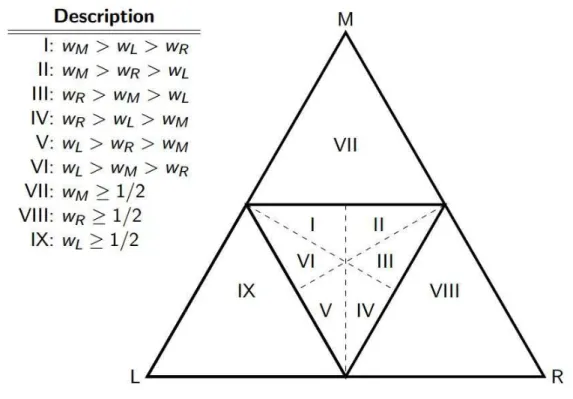
Considering that voters are discretely distributed across three ideologies (�, �
and�), we can illustrate any possible distribution as a point of a 2-simplex. Each vertex
of the triangle below represents an ideology and its corresponding height represents the
proportion of this group within the population of voters.
If all groups of voters choose a sincere behavior in the elections, the share of votes
obtained by a party will be equal to the proportion of its ideology in the population, i.e.
�� =à�,∀� ∈ ¶�, �, �♢. Hence, the simplex below can illustrate any conĄguration of the
legislature in the case of sincere voting:
Figure 1 Ű ConĄgurations of the legislature.
The regions in which �� ⊙1/2 for some� ∈ ¶�, �, �♢illustrate the cases in which
some party has the majority of the house. The other areas are the cases where parties
have to form a coalition through a bargaining process.
We suppose that only groups of voters with the extreme ideologies, � and�, show a sincere behavior during elections. Voters with ideal policy �� are able not only to
to coordinate their votes and determine the house composition from a set of possible
regions.
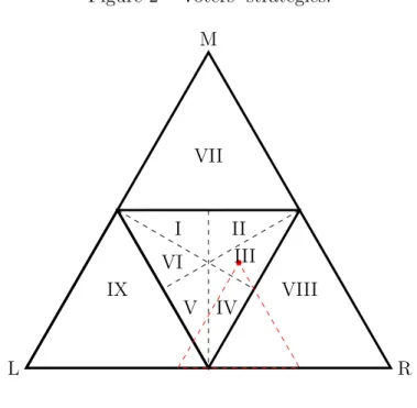
Consider for instance the case in which the proportion of ideologies between
voters is represented by the red point in Figure 2. If all voters choose a sincere behavior
at the elections, this point would also represent the legislature conĄguration, and the
government policy would be the equilibrium of the bargaining game given societyŠs
ideological distribution. However, voters with �� as the ideal policy can strategically
modify the house conĄguration to any other region below the red lines, since��⊙à� and
��⊙à� from our assumptions.
Figure 2 Ű VotersŠ strategies.
L
M
R IX
VII
VIII
I II
III
IV V VI
Since votersŠ utility depends on the government policy, and not on the policy
defended by the party for which they choose to vote, the group that behaves strategically
will decide their vote by choosing the region for which the optimum government policy is
closer to their ideal.
The set of possible choices depends on the votersŠ distribution of ideologies:
• If ideology � is the majority in the population (region VII), they can support any
• If some extreme ideology has the majority in the population (region VIII or IX), they
cannot change the legislative conĄguration, since they cannot decrease the share of
voters obtained by the party that represents the extreme ideology;
• If ideology � has the lowest representation in the population (region IV or V), this group of voters can only modify the legislative conĄguration to some other region
where they remain the minority (IV, V, VIII and IX);
• If � is the intermediate group of voters (region III or VI), besides the same options
available in the previous case, they can also choose their original region (for instance,
by voting sincerely);
• If ideology� has the largest representation in the population (region I or II), there will be two possible set of choices depending on the relation between the proportions:
– If votersŠ distribution is such that the presence of the second greatest ideology
is bounded between 1/4and 1/3, they can change to any region of the simplex;
– If the proportion is such that the presence of the second greatest ideology is
bounded between 1/3 and à�, they can give the majority to an extreme party (�or�), change to some region where they are minority (IV and V), strengthen the presence of a extreme party (� or�, the one that has higher participation), but remain as the intermediate (VI and III), or decide for a sincere behavior.
The analysis should consider the size of�and the ideological distances, since those elements impact the equilibrium of the government policy in each region and the group
with ideology � will choose the conĄguration that yields the government policy that maximizes their utility.
for the welfare analysis in the next chapter. The optimum strategies of voters with ideal
policy� = 0 are also described in the last column of those tables.1
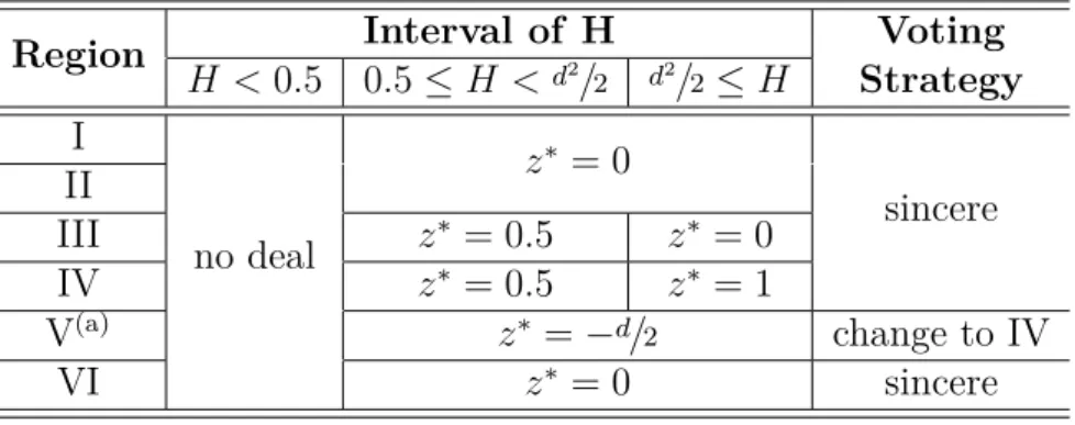
Table 3 Ű Strategy of voters with ideal policy � = 0 for 3⊘d.
Region Interval of H Voting
� <0.5 0.5⊘� <�2/
2 �2/2⊘� Strategy I
no deal
�∗ = 0
sincere II
III �∗ = 0.5 �∗ = 0
IV �∗ = 0.5 �∗ = 1
V(a) �∗ =
⊗�/2 change to IV
VI �∗ = 0 sincere
(a) In the specific case where�= 0.5, the optimum government policy will be�∗=−d/√2. However, the voting strategy is
still to move to region IV.
Table 4 Ű Strategy of voters with ideal policy� = 0 for 2<d<3.
Region Interval of H Voting
� <0.5 0.5⊘� <�2/
2 �2/2⊘� Strategy I
no deal
�∗ = 0
sincere II
III �∗ = 0.5 �∗ = 0
IV �∗ = 0.5 �∗ =(�−1)/2
V(a) �∗ =⊗�/2 change to IV
VI �∗ = 0 sincere
(a) In the specific case where�= 0.5, the optimum government policy will be�∗=−d/√
2. However, the voting strategy is
still to move to region IV.
1
The cases where 1> dare analogous, one would only need to exchange regions I and II, III and VI,
Table 5 Ű Strategy of voters with ideal policy � = 0 for √2<d ⊘2.
Region Interval of H Voting
� <0.5 0.5⊘� <�2/
2 �2/2⊘� Strategy I
no deal
�∗ = 0
sincere II
III �∗ = 0.5 �∗ = 0
IV �∗ = 0.5
V(a) �∗ =
⊗�/2 change to IV
VI �∗ = 0 sincere
(a) In the specific case where�= 0.5, the optimum government policy will be�∗=−d/√2. However, the voting strategy is
still to move to region IV.
Table 6 Ű Strategy of voters with ideal policy� = 0 for 1⊘d⊘√2.
Region Interval of H Voting
� <0.5 0.5⊘� <�2/
2 �2/2⊘� Strategy I
no deal
�∗ = 0
sincere II
III �∗ = 0.5 �∗ = 0
IV �∗ = 0.5
V �∗ =⊗�/2 change to IV
VI �∗ = 0 sincere
The votersŠ strategies are deĄned by choosing the region in which the government
policy is the closest to their ideal, given the set of possible choices and considering this
group of votersŠ utility,�� =⊗�⊗(�⊗��)2. Applying a variable transformation, we
can rewrite this utility as: �M/(�R)2 =� =⊗�⊗�2.
The main conclusions of this stage are:
1. If voters with the ideal policy � = 0 have the greatest presence in the population (region I or II), this group will vote sincerely. In this case, the party that represents
their ideology has enough bargaining power to support its ideal policy as the
government policy.
for the distance settings considered for the tables above), this group will also prefer
a sincere behavior in the elections. In spite of the coalition being formed between the
two extreme parties, the party that represents their ideology � = 0 at the legislature will have a great impact on the optimum proposal. Due to its advantage of being the
second proposer and the greatest party having an extreme ideology, more distant
from the other parties, the party with ideal policy � = 0 can lead the equilibrium to
its ideal.
3. If voters with ideal policy � = 0 have the second greatest presence in the population and the largest group is ideologically closer to them (region III for the distance
settings considered for the tables above), they will have the same advantage described
in the previous item. However, it is important to highlight that a decrease in the
bargaining resources � can lead to a government policy more distant from their ideal policy, since the bargaining power of the party that represents them will also
decrease. The greater the distance from the lowest party to the other two, the greater
the magnitude of � that is needed to ensure the advantage of their party.
4. Suppose now that voters with ideal policy � = 0 have the lowest presence in
population. They will always choose a strategy that increases the participation of the
ideologically closest party at the legislature and give them the greatest participation
in the house. Hence, they can lead the optimum proposal to a government policy
that is closer to their ideal policy.
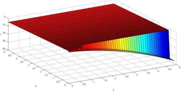
Figure 3 Ű Utility function over regions I, II and VI of the distribution of ideologies within the population.
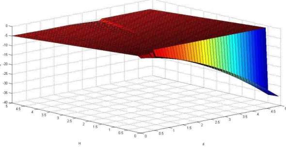
Figure 5 Ű Utility function over regions IV and V of the distribution of ideologies within the population.
We can identify in these Ągures the intervals of� and ideological distance ration
� and their efect on the utility of voters with intermediate ideology. An increase in �
can improve this groupŠs utility since it increases the bargaining power of the party that
represents their ideal policy in the legislature and then the government policy can get
closer to their ideal point. However, when this group has the lowest presence in society
(Figure 5), there is an interval for �∈[2,3] in which the magnitude of � that supports the optimum government policy depends on�. For this interval of the ideological distance ratio, we note that the lower �, the lower the magnitude of � necessary to support that government policy.
Notice that for �∈(0,1] the magnitude of � that supports an agreement between parties will depends on the relative distance between ideologies regardless the distribution
of ideology on the population. Therefore, the magnitude of � decrease as the relative distance of the left ideology � get smaller.
5 Social Welfare
In this chapter, we perform a welfare analysis for each region of the ideological
distribution of voters. Previously, we observed diferent efects of the magnitude of resources
present in the legislature (�) on the behavior of parties in the coalition formation process and on the utility of voters that behave strategically by anticipating post-election results.
The magnitude of legislative resources directly favors the party with the largest
participation in the house. However, it also increases the bargaining power of the other
parties present in the house, since all upcoming optimum proposals are anticipated by the
proposer.
Regarding the votersŠ behavior, it is considered that they are able to anticipate the
government policy from the legislative stage equilibrium. However, the strategic behavior
of voters with ideal policy � = 0 increases their utility only in cases where this group represents a minority of voters. The magnitude of � does not afect the electoral behavior of the strategic group, but interferes with their utility by its efect on the equilibrium
government policy.
Considering the aggregate of utilities of all voters, the social welfare function is
deĄned as:
� = (à�)
︁
⊗�⊗(�)2⎡+ (à�)
︁
⊗�⊗(�+�)2⎡+ (1⊗à� ⊗à�)
︁
⊗�⊗(�⊗1)2⎡
where à� eà� are the proportions of voters with ideology� and �in the population.
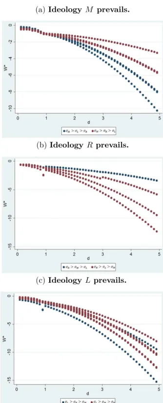
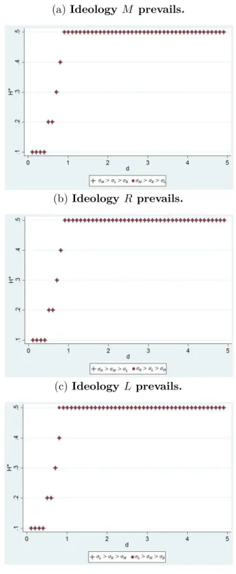
Figure 6 shows the optimum social welfare obtained for diferent ideological distance
Figure 6 Ű Optimum Social Welfare (�∗) depending on ideological distance (�),
considering diferent ideological distribution of voters
(a) Ideology M prevails.
(b)Ideology R prevails.
(c) Ideology L prevails.
We can observe from this Ągure a intuitive result. A higher relative distance between
the two most dominant ideologies in population gives a lower social welfare in cases that
presence in population, this result will depend on its proportion.
Regarding now the value of � that leads to those optimum social welfare, it will
depend on the ideological distance setting. This result is indicated at the Figure 7 below.
The pattern of maker also indicates which ideology is prevalent in population.
We can see that the optimal legislative resources �* is the same for all ideological distribution in population. It thus depends only on the relative distance of votersŠ ideology.
However, in all cases, it is only necessary to set a minimum value of� that supports an agreement between parties. When the relative distance between partiesŠ ideologies decreases,
i.e. parties get closer in terms of ideology, the magnitude of� necessary to support an agreement between these parties is smaller, regardless of the ideological distribution of
voters. These results are summarized in terms of the original variables at the following
proposition.
Proposition 2. Setting a value of �� to 1, the optimal legislative resources �∗ will not
depend on the ideology distribution in population. It will be depends only on the magnitude
of ��, such that:
1. for 0< ��<1, �∗ =(�L)2/2; and
2. for 1<=��, �∗ is limited by 0.5.
Therefore, the optimal legislative resources will be positively related to the ideological
Figure 7 Ű Optimum Financial Funding (�∗) depending on ideological distance (�),
considering diferent ideological distribution of voters
(a) Ideology M prevails.
(b)Ideology R prevails.
6 Conclusion
Our main conclusions can be classiĄed in three categories. We summarize the
impact of a resource restriction on the legislative outcome:
1. When the party with intermediate ideology is the largest in the house, it will be able
to form, together with the smallest party, a coalition that supports its ideal policy as
the government policy. The magnitude of the resources of the legislature will impact
only the conditions in which the agreement will be possible. Thus, there will be an
amount necessary for the coalition formation. If this amount is not achieved, no
agreement will be set.
2. When the party with intermediate ideology is the second largest, the largest in
the legislature will prefer to make a coalition with the smallest one, regardless of
the ideological distances between them. A decrease in the magnitude of legislative
resources can lead to a government policy closer to the largest partyŠs ideology. It
can beneĄt this group, but the impact on social welfare is ambiguous. Actually, it
may depend on the ideological distances setting.
3. When the party with intermediate ideology is the smallest, a decrease in the
mag-nitude of resources can sometimes improve the utility of the majority of voters by
leading to a government policy closer to their ideal policy. However, this impact
of the legislative resources on the government policy depends on the ideological
distances.
Regarding the votersŠ behavior, strategical voting is adopted only for cases in which
the group of voters with intermediate ideology has the lowest presence in the population.
We have also identiĄed how magnitude of resources in proportion to the ideological distance
setting afect the utility of the strategical voters.
An increase in legislative resources proportion can improve this groupŠs utility since