DEPARTAMENTO DE ENGENHARIA DE TELEINFORM ´ATICA
PROGRAMA DE P ´OS-GRADUAC¸ ˜AO EM ENGENHARIA DE TELEINFORM ´ATICA
ANA FL ´AVIA PAIVA RODRIGUES
DEFORMED EXPONENTIALS AND FINANCIAL MARKETS: APPLICATIONS TO PORTFOLIO SELECTION AND ASSET PRICING
DEFORMED EXPONENTIALS AND FINANCIAL MARKETS:
APPLICATIONS TO PORTFOLIO SELECTION AND ASSET PRICING
Tese apresentada ao Programa de P´os-Gradua¸c˜ao em Engenharia de Telein-form´atica do Departamento de Engenharia de Teleinform´atica da Universidade Fede-ral do Cear´a, como parte dos requisitos necess´arios para a obten¸c˜ao do t´ıtulo de Doutor em Engenharia de Teleinform´atica.
´
Area de concentra¸c˜ao: Sinais e Sistemas.
Orientador: Prof. Dr. Charles Casimiro Ca-valcante
FORTALEZA
Gerada automaticamente pelo módulo Catalog, mediante os dados fornecidos pelo(a) autor(a)
R611d Rodrigues, Ana Flávia Paiva.
Deformed exponentials and financial markets : Applications to portfolio selection and asset pricing / Ana Flávia Paiva Rodrigues. – 2018.
116 f. : il. color.
Tese (doutorado) – Universidade Federal do Ceará, Centro de Tecnologia, Programa de Pós-Graduação em Engenharia de Teleinformática, Fortaleza, 2018.
Orientação: Prof. Dr. Charles Casimiro Cavalcante.
1. Seleção de carteiras. 2. Modelos de fator único. 3. Exponenciais deformadas. 4. Divergências estatísticas. 5. Curvas principais. I. Título.
DEFORMED EXPONENTIALS AND FINANCIAL MARKETS:
APPLICATIONS TO PORTFOLIO SELECTION AND ASSET PRICING
Thesis presented to the Graduate Program in Teleinformatics Engineering of the Depart-ment of Teleinformatics Engineering of the Federal University of Cear´a in partial fulfill-ment of the requirefulfill-ments for the degree of Doctor of Philosophy in Teleinformatics En-gineering. Research area: Signals and Sys-tems.
Approved in: 28/03/2018.
THESIS COMMITTEE
Prof. Dr. Charles Casimiro Cavalcante (Advisor) Federal University of Cear´a (UFC)
Prof. Dr. Guilherme de Alencar Barreto Federal University of Cear´a (UFC)
Prof. Dr. Paulo Rog´erio Faustino Matos Federal University of Cear´a (UFC)
Prof. Dr. Aline de Oliveira Neves Panazio Federal University of ABC (UFABC)
First and foremost, I would like to thank God and St. Francis of Assisi, to whom I am devoted, for the enlightenment and blessings in this long and winding road.
To my husband, Jorge Lira, for his support and encouragement. To my son, Tom´as Paiva de Lira, a wonderful gift in my life! To my mother, Francisca Paiva, for her unconditional love everyday in my life. To my father, in memoriam, Manoel Ribeiro Rodrigues, for his admirable efforts in a life history dedicated to his family.
To my advisor, Charles Casimiro Cavalcante, for his guidance and confidence in this project. To my professors and colleagues in the Graduate Programs of Economics and Teleinformatics Engineering, for the uncountable learning opportunities. To professor Davi M´aximo, advisor in the split site doctoral program in Stanford University, for the opening of new opportunities.
To the members of the thesis committee, professors Guilherme Barreto, Paulo Matos, Aline Panazio and Renato Lopes, for the valuable suggestions and questions that considerably improved this work.
Propomos, neste trabalho, modelo de sele¸c˜ao de carteiras de ativos financeiros via um crit´erio de m´edia-divergˆencia, adaptado a retornos com distribui¸c˜oes dadas por exponen-ciais deformadas. Fixado o retorno esperado desejado, trata-se de minimizar o prˆemio de risco definido em termos de uma divergˆencia estat´ıstica. No caso de retornos gaus-sianos, a abordagem proposta reduz-se ao cl´assico modelo de m´edia-variˆancia concebido por H. Markowitz. Na sequˆencia, reformulamos o m´etodo de apre¸camento por proje¸c˜oes ortogonais desenvolvido por Luenberger para o contexto de m´ınima divergˆencia, o que nos permite propor modelos de fator ´unico, dentre os quais uma variante do CAPM com betas dependendo de uma matriz de covariˆancia generalizada. Os valores principais dessa matriz nos permitem, por fim, definir e aplicar uma no¸c˜ao estendida de curvas principais, o que adapta os conceitos desenvolvidos por Hastie e Stuetzle ao caso de exponenciais deformadas e divergˆencias de Bregman.
In this work, we propose a portfolio selection model based on a mean-divergence crite-ria, adapted to financial returns distributed according deformed exponential probability densities. Fixed a desired expected return, the method reduces to the minimization of a risk premium defined in terms of a statistical divergence, In the particular case of Gaus-sian returns, we recover the classical mean-divergence model by H. Markowitz. Next, we reformulate the projection pricing theory by Luenberger in the context of divergences as risk measures. This allowed us to define single factor models, including a variant of the CAPM whose beta coefficients depend on a Fisher metric that plays the role of a gene-ralized covariance matrix. The eigenvalues of this matrix are used to define an extended notion of principal curves that adapts the work by Hastie and Stuetzle to the case of deformed exponentials and their correspondent Bregman divergences.
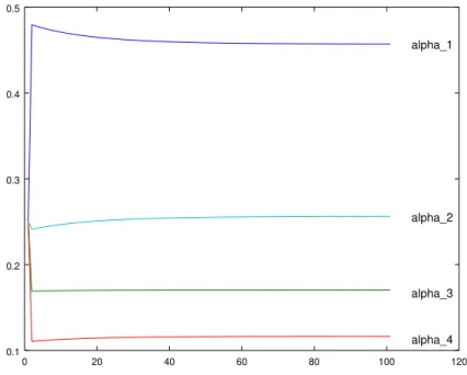
Figure 1 – Temporal evolution of weightsα1, . . . , α4 for the q-portfolio method. . . . 74 Figure 2 – Cumulated returns for proposed method (q-portfolio) and Markowitz’s
1 INTRODUCTION . . . 10
2 MODERN FINANCE THEORY: A SHORT REVIEW . . . 14
2.1 Utility and equilibrium . . . 19
2.2 Optimal portfolios . . . 28
2.3 Mean-variance analysis . . . 32
2.4 Projection pricing . . . 35
2.5 Beta models and Capital Asset Pricing Model . . . 38
3 FUNDAMENTALS OF INFORMATION THEORY . . . 41
3.1 Statistical divergences and Fisher metric . . . 45
3.2 Deformed exponentials . . . 48
3.3 Some technical computations . . . 51
4 MEAN-DIVERGENCE PORTFOLIO SELECTION . . . 64
4.1 Generalized HARA utility functions . . . 64
4.2 Generalized mean-divergence model . . . 65
4.3 Generalized Markowitz portfolio selection . . . 67
4.4 A natural gradient search . . . 71
4.5 Numerical examples and analysis . . . 73
4.6 A technical appendix . . . 77
5 SOME GENERALIZATIONS OF CAPM . . . 79
5.1 The space of financial assets . . . 79
5.2 Deformed exponentials and optimal φ-portfolios . . . 80
5.3 Notation and main results . . . 82
5.4 Geometry of statistical divergences . . . 85
5.5 Minimum divergence portfolio . . . 92
6 PRINCIPAL CURVES AND PORTFOLIOS . . . 99
6.1 Statistical divergences and principal curves . . . 99
6.2 The space of financial assets . . . 102
6.3 Generalized beta pricing models and CAPM . . . 107
6.4 Generalized PCA and applications to Finance . . . 109
7 CONCLUSION AND DEVELOPMENTS . . . 112
1 INTRODUCTION
The formulation of a non-extensive Statistical Physics by C. Tsallis (35), (36) and collaborators has been developed along the last two decades in a wide range of applications to complex systems, particularly in Finance (37), (38), (7), (40). In this work, we propose a model of portfolio selection of financial assets that explores the non-additivity and non-normality aspects of Tsallis’ Thermostatistics.
As highlighted by J. Naudts, deformed exponentials play a central role in the foundations of that Generalized Thermostatistics. Indeed, Naudts’ work established deep and fruitful connections between Statistical Physics and Information Geometry, (24), (25), (26), (27). For instance, both R´enyi’s and Tsallis’ entropies are described by Naudts in terms of statistical divergences in the family ofq-exponential distributions that includes
q-Gaussian distributions, defined in details by A. Plastino and C. Vignat (32), (33), (27), (28), (29). The analytic and geometric features of deformed exponentials suggest that they are well suited to model non-normally distributed returns of financial assets. In this direction, for instance, a non-Gaussian option pricing theory has been successfully proposed in terms of diffusion processes associated to q-Gaussian distributions (7), (8), (9), (40), (22). Other related developments are summarized in (38), (39).
Up to our knowledge, however, a systematic theory of portfolio optimization in the context of deformed exponentials has not yet been fully formalized. One of the cor-nerstones of the modern Finance Theory, the classical Markowitz’s mean-variance model of portfolio selection relies on the assumptions that the returns of assets are normally dis-tributed and that the investor preferences are described by constant risk aversion utility functions, see Section 2.1.
The traditional criticism to the normality assumption in Markowitz’s theory raises the need of alternative models for dealing with non-Gaussian distributions. This question has been addressed since the earlier developments of the Quantitative Finance under different methods. In (30), (31), R. Nock et al. extended the Markowitz’s mo-del to the wider family of exponential distributions, replacing the mean-variance by a mean-divergence model. Bregman divergences replace the variance as risk measures for non-Gaussian distributions, eventually encompassing information from higher order mo-menta. On the other hand, since statistical divergences define geometric measures on the statistical manifold of exponential distributions, their method has a geometric interpre-tation in terms of a steepest descent by the natural gradient of the risk premium (1), (3).
presentation of the Classical Portfolio Selection Theory, needed to guarantee a precise statement of our results. In Chapter 4 we extend the mean-divergence model in (30), (31) to deformed exponentials families. This part of the thesis is structured as follows. Earlier in Section 3.2 we recall basic notions and facts on the statistical manifold of deformed exponentials. We refer the reader to (1) for a comprehensive mathematical description of these manifolds. We also briefly describe in Section 4.1 a generalized family of hyperbolic risk aversion (HARA) functions as the natural choice of utility functions associated to returns with deformed exponential distributions. The mean-divergence model is presented in Section 4.2 as an extension of both Markowitz and R. Nock el al. models. Theorem 4.1 in Section 4.3 states that the optimal portfolio for the generalized mean-divergence model is given by a closed expression involving the information metric, that is, the Hessian of the cumulant function of the deformed exponential family. In the particular case of
q-Gaussian distributions, the optimal portfolio is explicitly given by
α= Σ
−1
q 1 1⊤Σ−1
q 1
,
where Σq stands for theq-Gaussian variance, which corresponds to the variance-covariance matrix in the Gaussian case. This theorem motivates the steepest descent algorithm by the natural (Riemannian) gradient of the risk premium in Section 4.4. Our method differs from the one in (30), (31) in some relevant aspects. For instance, the iterations in the search algorithm are indeed defined in terms of the projection of the natural gradient on the simplex of admissible portfolios. Moreover, we stress the fact that this machine learning procedure stems naturally from the generalized Markowitz’s formula in Theorem 4.1 what provides an analytical justification that was not entirely evident in (30), (31). Some empirical support to the proposed method is discussed in Section 4.5. There we compare the cumulated returns and the evolution of the divergence for optimal portfolios according to the mean-divergence model and the classical one by Markowitz. Chapter 4 finishes with a brief discussion of prospective empirical tests and theoretical developments. Chapter 5 is a natural sequel of Chapter 4 in the sense that we propose a generalization of beta pricing models adapted to a mean-divergence portfolio selection (34), (17), (23). In particular, we present an extension of Capital Asset Pricing Model (CAPM) flexible enough to be applied for financial returns with deformed exponential distributions. Our method relies on a geometric approach to the classical mean-variance analysis developed by S. LeRoy and J. Werner (16) and D. Luenberger (19), see also (13). We refer the reader to (6) to a precise and comprehensive exposition of the classical CAPM model.
This chapter begins with the definition in sections 5.1 and 5.2 of the geometric setting of the space of contingent claims M and the subspace of traded financial assets
-deformed exponentials. Some geometric features of that manifold are summarized in Section 5.4. Following (16), we define expectation and price kernels in terms of a Bregman statistical divergence in M. These two distinguished assets span the mean-divergence efficient frontier inM′. As in (30), (31) and (10), the underlying idea is that the divergence
defined a novel risk measure that replaces the variance in the case of normal distributions. Taking this into account, we deduce in Section 5.5 an expression of a minimum divergence portfolio in the efficient frontier. Roughly speaking, the efficient frontier is the set of tradable assets with the minimum risk among those with the same expected return. As in the classical beta pricing models, the proportions of market portfolio and risk-free assets in this optimal portfolio are dictated by a linear regression coefficient
β =− g(Rq−Re, Re)
g(Rq−Re, Rq−Re)
, (1)
where Rq and Re correspond to the market return and risk-free return in the standard
beta pricing equation. Here, g stands for the Riemannian metric in M′ given by the
Hessian of the cumulant function K of the deformed exponential probability density. In the classical case of Gaussian distributions, we have a flat metric given by the variance. In our general approach, the Riemann curvature of M′ encodes third and fourth order
moments of the distribution as follows from equation (300). Using this machinery, one can obtain further developments for applications of the theoretical model deduced in this work. Some prospective directions are related to estimation techniques of the generalized beta factors, specially useful for valuation models in Corporate Finance.
Now, we briefly discuss the contents of Chapter 6. In their seminal paper (14), T. Hastie and W. Stuetzle proposed a notion of principal curves as an elegant and geometric non-linear generalization of factor models as the principal component analysis. A principal curve has the property of self-consistence in the sense that it pass through the middle of the data set representing a sample of some random variable. More precisely, any point of the curve coincides with the expected value of the data projected on it. This is a direct consequence of the fact that a principal curve f is critical for the variance of the Euclidean distance between the data and any locally defined perturbation of f. In particular, a straight line is a principal curve if and only if its direction is an eigenvector of the covariance matrix of z.
is, the variance used in the original definition.
Considering statistical divergences as Kullback-Leibler or Bregman divergence allows us to deal with random variables whose probabilities are given by exponencial and deformed exponential distributions. In the context of exponential andφ-exponential statistical families, straight lines are replaced by affine geodesics and the Hessian of the cumulant function plays the role of a generalized covariance.
2 MODERN FINANCE THEORY: A SHORT REVIEW
Financial assets, more precisely their payoffs at a fixed time, say t = 1, are represented by random variables of the form
z=z(s),
wheres are the states of the world with probability distribution specified by some density
p(s;ϑ). Here, ϑ is the distribution parameter of a family of probability distributions whose densities define an-dimensional statistical manifold
S ={p(s,ϑ) :ϑ ∈U ⊂Rn},
withϑ = (ϑ1, . . . , ϑn) taking values in some open subsetU of then-dimensional Euclidean space Rn. Given a time series of payoffs {z(i)(s)}T
i=0 one defines the returns of the asset
as the percentual ratio
r(i+1)(s) = z
(i+1)(s)−z(i)(s)
z(i)(s) (2)
fori= 0, . . . , T −1.
Example 2.1 It is an usual however possibly unrealistic assumption that the returns of a financial asset are (log)-normally distributed. This means that the random variable r(s) has a Gaussian distribution whose density is of the form
p(s, µ, σ) = 1 (2π)12σ
exp
− 12(r−µ)2 1
σ2
,
where µ ∈ R and σ2 ∈ R+ are, respectively, the mean and variance of the distribution.
If one considers N financial assets, then it is commonly supposed that their returns are distributed according to a multivariate Gaussian distribution with density given by
p(s,ϑ) =p(s, µ,Σ) = 1 (2π)N2|Σ|12
exp
− 1
2(r−µ)
TΣ−1(r−µ)
.
Note that in those examples the parameters ϑ = (ϑ,Θ) ∈ RN ×M(N,R) are explicitly
given by
ϑ= Σ−1µ∈RN
and
Θ = 1 2Σ
−1
∈M(N,R),
where µ∈RN and Σ∈M(N,R) are, respectively, the mean and the covariance matrix of the distribution.
determine a subset of a larger family of probability distributions, namely an exponential family.
We refer the reader to (6) and (12) as comprehensive and formal presentations of the main aspects of Finance Theory.
One of the fundamental principles in Modern Finance Theory is the No Ar-bitrage Theorem whose far reaching consequences encompass the whole theory of asset pricing. As a simpler version of the No Arbitrage Theorem, we restrict ourselves to con-sider a risky asset with payoffz(s), an option c(s) whose underlying asset payoff isz and a risk-free asset 1. This last notation indicates that this asset yields the same risk-free return, say r, in every state of the world, that is, under any circumstances. On the con-trary, both z(s) and c(s) are by definition sensitive to the effect of distinct states of the world. Supposing by the sake of simplicity that there are two different states of the world, we can arrange all the possible payoffs in a matrix as
D=
1 +r 1 +r z(1)(down) z(1)(up) c(1)(down) c(1)(up)
LetQ be the vector of current market values (at time t= 0) of these securities, that is,
Q=
1
z(0) c(0)
The possible returns ofz are given by
r(down) = z
(1)(down)−z(0)
z(0) and r(up) =
z(1)(up)−z(0)
z(0) ·
We distinguish between these two scenarios declaring that
r(down)< r(up).
Suppose that
r < r(down)< r(up). (3)
In this case, an investor could get a long position in the assetz buying shares of it with money borrowed at a risk-free rate r, a sort of financial leverage. Even in the worst scenario, (3) implies that the investor would obtain positive returns at time t= 1. Now, under the assumption that
r(down)< r(up) < r, (4)
is, selling shares of z and investing in the risk-free security. We conclude that if either (3) or (4) are valid, then there are arbitrage possibilities in the market: in both cases, it is characterized the existence of a portfolio composed by the risky asset and the risk-free security that costs nothing to the investor and, in spite of that, yields positive returns.
Those arbitrage opportunities are ruled out by imposing that
r(down)< r < r(up). (5)
This condition has important implications on the pricing of the risky assets as we will see in the sequel. We would like to prove the existence of a state-price vector π = (π(down), π(up)), that is, a vector with positive components for which it holds that
Q=D π,
that is,
1
z(0) c(0)
=
1 +r 1 +r z(1)(down) z(1)(up) c(1)(down) c(1)(up)
"
π(down)
π(up) #
.
Then we would like to guarantee the existence of positive solutions to the system of linear equations
(1 +r)π(down) + (1 +r)π(up) = 1
z(1)(down)π(down) +z(1)(up)π(up) =z(0), (6)
or, equivalently,
(1 +r)π(down) + (1 +r)π(up) = 1
(1 +r(down))π(down) + (1 +r(up))π(up) = 1, (7)
with π(down)>0, π(up)>0. Subtracting the first equation from the second, we have
(r(down)−r)π(down) + (r(up)−r)π(up) = 0
Hence, in order to get positive solutions, a sufficient and necessary condition is
r(down)< r < r(up),
Note that the first equation in 6 implies that the components
b
π(down) = (1 +r)π(down), πb(up) = (1 +r)π(up) (8)
can be interpreted as set of probabilities, referred to as therisk-neutral probabilities. The second equation in 6 may be written in terms of this notation as
z(0) = 1 1 +r z
(1)(down)
b
π(down) +z(1)(up)bπ(up),
that is,
z(0) =Eπb
1 1 +rz
(1)
. (9)
This last equation asserts that the current market value of a risky asset is given, in the absence of arbitrage opportunities, as the expected value of the payoffs of this asset, discounted at a risk-free return data, where the expectation is calculated with respect to risk-neutral probabilitiesπb.
Note that, intuitively, z(s) does not behave as in (9) if one considers actual subjective probabilities since the expected return of a risky asset must exceed the risk-free return, that is,
z(0) <E
1 1 +rz
(1)
if the expectation is computed with respect to some set of subjective probabilities. This last inequality means that the discounted (with respect to a risk-free rate r) expected subjetive return of a risky asset must be positive in order to motivate an investment decision.
We have ignored so far the consequence of the existence of a state-price vector
π on the option pricing. It follows from our earlier considerations that c(s) also satisfies the condition
c(0) =Eπb
1 1 +rc
(1)
. (10)
This is the starting point of the binomial method of option pricing proposed by Cox, Ross and Rubinstein. In the limit, that binomial process restores the celebrated Black-Scholes-Merton formula for option pricing in the context of time continuous stochastic processes.
Now we state the No Arbitrage Theorem in a more general setting. We par-tially follow here the terms and notations in (12). In the general case of N securities
z1(s), . . . , zN(s), a portfolio is defined by an allocation vector
α= (α1, . . . , αN)∈RN (11)
say) on the asset zi. Supposing that we have only a finite set of states of the world Ω ={s1, . . . , sK}, we denote the payoff N ×K matrix by
D=
z1(s1) . . . z1(sK) ... . .. ...
zN(s1) . . . zN(sK)
The payoff portfolio is given by the random variable
αD=h α1z1(s1) +. . .+αNzN(s1) . . . α1z1(sK) +. . .+αNzN(sK), i
where the possible payoffs correspond to the time 1. The set of payoffs available via trades in security markets is the linear span of a basis of traded assetsz1, . . . , zN, that is,
M={z ∈RK :z =αD}. (12)
A market is said to be complete ifM=RK, that is, every possible payoffz ∈RK can be
replicated by a traded portfolio. This is equivalent to the condition that the rank ofD is exactlyK. In particular, N ≥K.
If the rank ofDisN (in particularN ≤K), there are no redundant portfolios: if there exist two portfolios inM with the same payoff, they are equal. Indeed, given α
and α′ such that
αD=α′D
then
(α−α′)D= 0.
Since the rank ofD is N, it defines an injective linear map and then
α=α′.
Given the current value market, that is, the price vector of all the traded assets
Q=
z(0)1
...
z(0)N
the price of a portfolio αis
hQ,αi= N X
i=1
zi(0)αi.
Definition 2.1 An arbitrage portfolio α∈RN satisfies by definition one of the following
i. hQ,αi ≤0 and αD(s)>0 for every s∈Ω. ii. hQ,αi<0 and αD(s)≥0 for every s∈Ω.
According to this definition, the arbitrage portfolioαcan be purchased without (respectively, negative) costs and guarantees some positive (respectively, nonnegative) return in all states of the world.
Theorem 2.1 (Fundamental Theorem of Finance Theory) There is no arbitrage if and only if there is a state-price vector π(s)>0 such that
Q=D π. (13)
For a proof of this theorem, we refer the reader to (12), p. 10.
As above we define risk-neutral probabilities from the state-price vector: de-note
π0 =π1+. . . .+πN
and set
b
π = 1
π0 π
in such a way thatbπi >0 and b
π1+. . .+bπN = 1.
Hence
Qi = N X
j=1
πjDij = 1
π0
N X
j=1
b
πjDij =Ebπ
1
π0Di
,
recovering the fact that, using risk-neutral probabilities, the current price of an asset zi is given by the expected payoff, discounted at a risk-free rateπ0. Indeed, if there exists a risk-less asset 1 with same payoff in every state of the world s∈Ω, then
1·π1+. . .+ 1·πN = expected future value of 1= 1 +r,
wherer is the rate of return of the risk-less asset. Hence,
π0 = 1 +r.
2.1 Utility and equilibrium
An agent is characterized by an endowmente∈RK
+ and a differentiable strictly increasing
utility function
u:RK
+ →R
where
RK
Note thatcis a random variable depending on theK states of the world and representing the investor’s consumption choices. More generally, one may consider a utility function depending on the investor’s choices (consumption plans) at two distinct times, say t= 0 andt= 1. In other terms, we consider an utility function defined inR+×RK
+ of the form
u(c(0), c(1)).
Herec(0)≥0 andc(1) ≥0 are, respectively, the consumption plans of the investor at times t = 0 and t = 1. Both e and c are modelled as random variables e = e(s) and c =c(s) depending on the states of the world s ∈ Ω. We refer the reader to (6), (16), (18) for further details on the notions and fundamental results in this section.
Given consumption plans c, c− and c+ one has by assumption that
u(c(0)− , c(1))< u(c(0)+ , c(1))
if c(0)− < c(0)+ and
u(c(0), c(1)− )< u(c(0), c(1)+ )
if c(1)− < c(1)+ . The partial order for vectors (consumption bundles) in RK+ is defined here
by
c−< c+ if and only if c−i < c+i,
for everyi= 1, . . . , K. We then consider the following constrained optimization problem
max c,α u(c
(0), c(1)) (14)
subject to the constraints
c(0) ≤e(0)− hQ,αi (15)
c(1) ≤e(1)+αD (16)
Theorem 2.2 If there is no arbitrage, then the problem (14), (15)-(16) has a solution, that is, there exists an optimal consumption plan and optimal portfolio.
Proof. Without loss of generality, we may assume that there are no redundant portfolios. Indeed redundant portfoliosα and α′ have the same payoffs, that is,
αD=α′D.
Since there are no arbitrage portfolios, we conclude that α and α′ also have the same prices:
Then the maximization problem does not distinguish between redundant portfolios and then we may take only a representative of possible redundant portfolios. In technical terms, this means that we may consider the quotient space of the feasible set by kerD.
Sinceu is a continuous function, the optimization problem can be solved once we prove that the constraints define a closed and bounded subset inRK
+. Given admissible
sequences{cn}and {αn}of consumption plans and portfolio allocations, respectively, we have
c(0)n ≤e(0)− hQ,αni (17)
c(1)n ≤e(1)+αnD (18)
Ifcn→cand αn →αthen {c,α} lies in the feasible set, that is,
c(0) ≤e(0)− hQ,αi (19)
c(1) ≤e(1)+αD (20)
Therefore, the feasible set is closed. In order to prove that it is also bounded, suppose by contradiction that there exists anunbounded sequence {cn,αn} in the feasible set. This implies that the sequence of portfolios {αn} is unbounded. Otherwise, the constraint inequalities
c(0)n ≤e(0)− hQ,αni (21)
c(1)n ≤e(1)+αnD (22)
would imply that {cn} would be bounded too. Hence, {αn} is unbounded in the sense that
|αn|= (α21+. . .+αn2)1/2 →+∞
asn →+∞. On the other hand, since the consumption plans are non-negative, that is,
c(0)n ≥0 and c(1)n ≥0, we have
hQ,αni ≤e(0) (23)
−αnD≤e(1) (24)
Therefore, dividing both sides of the constraint inequalities by |αn| yields
D
Q, αn
|αn|
E
≤ 1
|αn|e
(0) (25)
− αn
|αn|
D≤ 1
|αn|
However a subsequence of
αn
|αn|
converges to some non-zero portfolio α∈RN. Taking limits on both sides of the
inequa-lities 25-26 above, one concludes that
hQ,αi ≤0 (27)
−αD≤0 (28)
Sinceα6= 0 and due to the fact that only the trivial portfolio has zero payoff, we conclude that
αD >0
with hQ,αi ≤ 0 what means thatα is an arbitrage portfolio. This contradiction proves that the feasible set is closed and bounded. This is enough to ensure the existence of an
optimal solution, finishing the proof.
Theorem 2.3 If there exist an optimal consumption plan and optimal portfolio for the problem (14), (15)-(16), then there is no arbitrage portfolio.
Proof. Suppose by contradiction that there exists an arbitrage portfolio α0. Then, given
any feasible consumption plan and portfolio {c,α}one has
hQ,α0i ≤0
(respectively,hQ,α0i<0) and
α0D >0
(respectively,α0D≥0.) In both arbitrage cases, one gets
c(0) ≤e(0)− hQ,α+α0i (29)
c(1) ≤e(1)+ (α+α0)D, (30)
that is,
c(0)+hQ,α0i ≤e(0)− hQ,αi (31)
c(1)−α0D≤e(1)+αD, (32)
Sinceuis strictly increasing and at least one of the inequalities above is strict, we conclude that the consumption plan (c(0)− hQ,α
0i, c(1)−α0D) is strictly preferred to the optimal
consumption plan (c(0), c(1)). This contradiction proves that there is no arbitrage portfolio,
finishing the proof.
of an optimal consumption plan and portfolio for investors whose utility functions are strictly increasing with respect to both present and future consumption plans.
The constrained maximization problem 14, 15-16 may be formulated in terms of the Lagrangian
L=u(c(0), c(1)) +λ(c(0)−e(0)+hQ,αi) +µ(c(1)−e(1)−αD) (33)
It follows that the first-order conditions (at a regular maximum point) are given by
∂c(0)u+λ= 0, (34)
∂c(1)u+µ= 0, (35)
λQ−µD= 0. (36)
Combining these equations gives
Q=D∂c(1)u ∂c(0)u
(37)
We conclude that the state-price vector π is given by the marginal rate of substitution, that is,
π = ∂c(1)u
∂c(0)u·
(38)
Equations 34-36 are also sufficient conditions to the optimality of some feasible {c,α}
in the case when the utility function is differentiable and concave, see (12), p. 13. The concavity assumption is also useful to guarantee the existence of a general equilibrium in securities market, see Theorem 1.8.1 in (16).
Theorem 2.4 If each agent’s admissible consumption plans are restricted to be non-negative, her utility function is strictly increasing and concave, her initial endowment is strictly positive, and there exists a portfolio with strictly positive payoff, then there exists an equilibrium in security markets.
An equilibrium in a market composed by M investors (u(ℓ),eℓ), ℓ= 1, . . . , M, andN assets with payoffs Dis by definition a state-price vectorπ and individual optimal allocationsαℓ,ℓ = 1, . . . , M, for (14), (15)-(16) such that
M X
ℓ=1
αℓ = 0 (39)
Expected utility
In this section, we restrict ourselves to the case of expected utility functions, a central concept in von Neumann and Morgenstern theory of choice under uncertainty. A detailed account of this theory and criticism may be found in (21) and (6). The theoretical appa-ratus of von Neumann and Morgenstern relies on a list of axioms, the most controversial being the independence axiom that states that consumption plans, represented by random variables of the form
c= (c1, . . . , cK)∈RK,
satisfy the preferences ordering relations
(c1, . . . , ci−1, x, ci+1, . . . , cK)%(c′1, . . . ,cˆ′i−1, x,ˆc′i+1, . . . , c′K)
if
(c1, . . . , ci−1, ci, ci+1, . . . , cK)%(c′1, . . . ,cˆ′i−1, c′i,ˆc′i+1, . . . , c′K)
for all c, c′ ∈ RK and x ∈ R. Here, A % B is a preference ordering that means that
“A is preferred to B”. Besides that, one of the main hypothesis in this theory is that expectations are calculated with respect to givenobjectiveprobabilities. Hence, a portfolio is described in terms of a “gamble”
(c1, p1), . . . ,(cK, pK)
,
that is, a given list of possible payoffs of the consumption plan and their respective probabilities.
It follows from that axiomatic approach that rational optimization under un-certainty could be modeled in terms of a particular form of the utility function that we are going to use in the sequel. Indeed, we consider in what follows the case of an expected utility function defined in terms of a set of probabilities{p1, . . . , pK} by
u(c(0), c(1)) =u0(c(0)) +E[u1(c(1))] = u0(c(0)) +
K X
j=1
pju1(c(1)(sj)). (40)
This means thatuis separated into two components, u0 and u1 that depend respectively on the consumption plans at times t = 0 and t = 1. Note that the function u1 does not depend on the parameter j, that is, does not depend on the states of the world sj ∈ Ω. In this case, condition 37 reads as
Q= 1
∂c(0)u0 K X
j=1
what implies that
Q= 1
∂c(0)u0
E[Du′
1(c(1))]. (41)
For the sake of simplicity we will assume for a while that u0 ≡ 1. An agent is said to berisk-averse if she prefers the expectation of any consumption plan to the consumption plan itself, that is,
E[u1(c(1))]≤u1(E[c(1)]), (42)
for every consumption plan c. Intuitively, the right-hand side u1(E[c(1)]) is the utility of
the expected value of the lottery represented by the random variable c(1). This is the
risk-less position to the investor. The left-hand side E[u1(c(1))] is the expected utility of
the lottery. The inequality means that, in order to move from the risk-less position to a riskier one, the risk-averse investor demands a positive risk premium that we are going to define shortly afterwards. For risk neutral agents instead, we have
E[u1(c(1))] =u1(E[c(1)]), (43)
for every consumption plan c. It turns out that an agent is risk averse (respectively, risk neutral) if and only if her von Neumann-Morgenstern utility function u1 is concave
(respectively, linear). This follows from Jensen’s inequality for concave functions. Indeed, if u1 is concave we have
p1u1(c(1)(s1)) +. . .+pKu1(c(1)(sK))≤u1(p1c(1)(s1) +. . .+pKu(1)(sK)),
that is,
E[u1(c(1))]≤u1(E[c(1)]).
The Jensen’s gap
J =u1(E[c(1)])−E[u1(c(1))]
increases with the concavity of the graph ofu1. This indicates that the second derivative of u1 encodes some information about the investor’s aversion to risk. Indeed, one of the commonly used risk measures is the Arrow-Prattabsolute risk aversion coefficient defined by
a=−u′′1(c
(1)) u′
1(c(1))
· (44)
We now define the risk premium, a notion that is closely related to Jensen’s gap. Let ¯c(1) be the mean of the random variable c(1), that is,
¯
Setting
c(1) = ¯c(1)+ε,
whereε is a random variable with zero mean, we define the risk premium Π by
E[u1(¯c(1)+ε)] = u1(¯c(1)−Π) (45)
The certainty equivalent is by definition
C = ¯c(1)−Π. (46)
The risk premium Π can be regarded as the maximum amount the investor renounce in order to avoid the “gamble” represented by the random factorε. We have for an arbitrary von Neumann-Morgenstern utility function the following approximation
u1(¯c(1)+ε) =u1(¯c(1)) +u′1(c(1))ε+ 1 2u
′′
1(c(1))ε2+O(ε3) (47)
and since E[ε] = 0 one gets
E[u1(¯c(1)+ε)]∼u1(¯c(1)) + 1
2u
′′(c(1))E[ε2].
up toO(ε3) remainder. Recall that the variance of ε is given by
var[ε] =E[ε2]−(E[ε])2 =E[ε2].
Therefore
E[u1(¯c(1)+ε)]∼u1(¯c(1)) + 1
2u
′′(c(1))var[ε].
On the other hand
u1(¯c(1)−Π)∼u1(¯c(1))−u′(¯c(1))Π
up to second order terms in Π. Then, we obtain the approximation
Π ∼ −1 2
u′′(¯c(1))
u′(¯c(1))var[ε] (48)
or, in terms of the risk aversion coefficient
Π∼ −1
2avar[ε] (49)
One deduces from (49) that i. Ifu′′
1(c(1))>0 thenC > u(c(1)) and the investor prefers a greater certainty equivalent
ii. Ifu′′
1(c(1))<0 thenC < u(c(1)) and the investor prefers a lower certainty equivalent
on an uncertain investiment than its expected value. iii. If u′′
1(c(1)) = 0 then C=u(c(1)) and the investor has a certainty equivalent equal to
the expected return.
In the special case of a CARA (constant absolute risk aversion) utility function one has
u′′ 1(¯c(1)) u′
1(¯c(1))
=−a
for some constanta. Hence u can be taken as
u1(¯c(1)) =−exp(−a¯c(1)). (50)
In this case we have
u1(¯c(1)−Π) =−exp(−ac¯(1)+aΠ) =−exp(−a¯c(1)) exp(aΠ).
We obtain in a similar way that
u1(¯c(1)+ε) =−exp(−a¯c(1)) exp(−aε)
from what follows that
E[u1(¯c(1)+ε)] = −exp(−ac¯(1))E[exp(−aε)]
Comparing both expressions, one obtains
exp(aΠ) =E[exp(−aε)].
At this point, suppose that the random deviationsε are normally distributed with mean
µand covariance matrix Σ. Using that E[ε] = 0 and denotingσ2 = var[ε] one has
E[exp(−aε)] = 1
(2π)12σ Z
exp
−aε− 1
2 1
σ2ε 2
dε
= 1
(2π)12σ Z exp − 1 2 1
σε+aσ
2
exp
1 2a
2σ2
dε
= 1
(2π)12σ Z exp − 1 2t 2 exp 1 2a
2σ2
σdt
= exp
1 2a
2σ2
1 (2π)12
Z exp −1 2t 2
dt = exp
1 2a
2σ2
incre-ments ε, we have exactly
Π = 1
2avar[ε]. (51)
The certainty equivalent in this case is given by
C=µ−1
2aσ
2, (52)
where
µ=E[c(1)].
2.2 Optimal portfolios
We refer the reader to (6), (16), (18) for further details on the notions and fundamental results in this section.
Suppose that c(0) = 0. We recast the optimization problem 14, 15-16 in the
context of expected utility function as
max
α′
E[u1(c(1))] (53)
subject to
e(0) =hQ,α′i, (54)
c(1) =e(1)+α′D. (55)
Suppose that the endowment at time t= 1 lies in the asset spanM. Then there exists a portfolio α0 such that
e(1) =α0D.
and the price of this portfolio generatinge(1) is given by
hQ,α0i.
Denoting
α′ =α−α0
we write 54 and 55 respectively as
e(0)+hQ,α0i=hQ,αi
and
In this case, we define the wealth of the investor by
w(0)=e(0)+hQ,α0i (56)
and recast the problem 53, 54-55 as
max
α
E[u1(αD)] (57)
subject to
w(0) =hQ,αi. (58)
According to this formulation of the problem, we can regard the portfolio payoff αD as the investor’s wealth at timet= 1, that is,
w(1) =αD. (59)
The Lagrangian associated to 57-58 is of the form
L=E[u1(αD)]−λ(hQ,αi −w(0)).
The first-order condition may be formally written as
E[u′
1(w(1))Di] =λQi (60)
for all i. Since
Di−Qi
Qi
=ri =:Ri−1
after dividing both sides by λQi one gets
E
1
λu ′
1(w(1))Ri
= 1 (61)
for all i. Therefore, given two assets with returnsRi and Rj we have
0 =E
1
λu ′
1(w(1))Ri
−E
1
λu ′
1(w(1))Rj
=E
1
λu ′
1(w(1))(Ri−Rj)
.
It follows that
E
1
λu ′
1(w(1))(Ri−Rj)
= 0.
Choosing one of the assets to be risk-free, say setting Rj =Rf, the risk-free return rate,
and obtain
E
1
λu ′
1(w(1))(Ri−Rf)
The random variable Ri−Rf is the excess return of the asset zi compared with the risk-free return. Applying 60 to a risk-risk-free asset with return Rf (that is, setting Ri = Rf in
60) one has
RfE
u′1(w(1))=Eu′
1(w(1))Rf
=λ
This determines λ in 60. Hence, considering again the expression 60 for an arbitrary Ri gives
E
1
λu ′
1(w(1))D
=Q (63)
is a stochastic version of the price law
D π =Q.
Then we refer to
m:= 1
λu ′
1(w(1)) =
1
Rf
u′ 1(w(1)) Eu′
1(w(1))
as astochastic discount factor playing a role similar to the state-price vectorπ. It follows from 61 that
E[mRi] = 1. (64)
On the other hand
E[mRi] =E[m]E[Ri] + cov[m, Ri]. (65)
Applying 64 to Ri =Rf one has
E[m]Rf = 1,
that is,
E[m] = 1 Rf·
This determines E[m] in terms of Rf. Replacing this expression in 65 yields
1
Rf
E[Ri] + cov[m, Ri] = 1.
Rearranging terms, one obtains
E[Ri]−Rf =−Rfcov[m, Ri] (66)
In order to fix ideas, we are going to perform some explicit calculation in the case of CARA utility function and normally distributed returns. We have in this particular setting that
u1(c(1)) =u1(w(1)) = −exp(−aαD).
variance respectively byµ and σ2. Then
µ=E[αD] =αD¯ and σ2 =αΣα⊤,
where ¯Dand Σ are, respectively, the mean vector and the covariance matrix of the payoffs
D. DenotingαD=z one has as above
E[u1(w(1))] = E[−exp(−aαD)]
=− 1
(2π)12σ Z
exp(−az) exp
− 1
2 1
σ2(z−µ) 2
dz
=− 1
(2π)12σ Z exp − 1 2
z−µ
σ +aσ
2
exp
1 2a
2σ2−aµ
dz
=− 1
(2π)12σ Z exp − 1 2t 2 exp 1 2a
2σ2
−aµ
σdt
=−exp
1 2a
2σ2
−aµ
1 (2π)12
Z exp
−12t2
dt =−exp
1 2a
2σ2
−aµ
=−exp
−a
µ− 1
2aσ
2
=u1
µ− 1
2aσ
2
.
We conclude that the certainty equivalent of the random wealthw(1) is given by
C=µ−1
2aσ
2, (67)
that is,
C =αD¯ − 1
2aαΣα
⊤, (68)
where Σ is the covariance matrix of the payoffs of the basic assets z1, . . . , zN. Hence the risk premium is completely determined by the variance of the portfolio and the absolute risk aversion coefficient:
Π = 1
2aαΣα
⊤. (69)
More importantly, we deduce that maximizing the CARA expected utility is equivalent to maximizing the utility of the certainty equivalent, which amounts to be equivalent to maximizing C itself. The corresponding first order condition is
¯
D−aαΣ = 0.
Therefore, the optimal portfolio is given by
α= 1
aΣ
2.3 Mean-variance analysis
The earlier computations motivate the problem of maximizing the certainty equivalent. As we have seen, under the assumption of CARA utility function and normally distributed returns this problem reduces to the mean-variance criterion for the choice of optimal portfolios:
max
α
αD¯ − 1
2aαΣα
⊤
(71)
Then we consider the mean-variance problem formulated by Harry Markowitz (20):
min
α αΣα
⊤ (72)
subject to
hα, Di=µ∗ (73)
hα,1i= 1, α≥0, (74)
whereµ∗ is the desired expected return for the portfolio. Note that here we are represen-ting D as a N-dimensional random vector (depending on K states of the world instead of aN ×K matrix. The second constraint implies that
α∈ SN−1 ⊂RN
whereSN−1 is the (N −1)-dimensional simplex defined by
SN−1 =
α= (α1, . . . , αN)∈RN : 0≤αi ≤1 and N X
i=1
αi = 1
First, we consider the Lagrangian
Lµ = 1 2αΣα
⊤−λ(hα, Di −µ
∗) (75)
subject to the restriction
hα,1i= N X
i=1
αi = 1. (76)
The first order condition is
αi =λ(DΣ−1)i =:λψi.
Then, considering the restriction 76 one has
λ
N X
i=1 ψi =
N X
i=1
Therefore
λ= PN1 i=1ψi
·
We conclude that the optimal portfolio is given by
αµ=
DΣ−1
hDΣ−1,1i· (77)
Next, we define the Lagrangian
L1 =
1 2αΣα
⊤−ν(hα,1i −1) (78)
subject to the constraint of prescribed expected portfolio return:
hα, Di=µ∗. (79)
Now, the first order condition is
αi =ν(1Σ−1)i =:νφi.
Note that as before
ν
N X
i=1 φi =
X
i=1
αi = 1
from what follows that the optimal portfolio forL1 is
α1 = 1Σ−
1
h1Σ−1,1i· (80)
In view of the restriction 79 one obtains
νhφ, Di=hα, Di=µ∗
what implies that
h1Σ−1, Diν =µ
∗ (81)
Similarly one gets
hDΣ−1, Diλ=µ∗. (82)
It follows that an optimal portfolio for the full Lagrangian
L= 1 2αΣα
⊤−λ(αD−µ
∗)−ν(hα,1i −1)
can be expressed as
that is,
α=eλ DΣ− 1
hDΣ−1,1i +eν
1Σ−1
h1Σ−1,1i (84)
where the coefficientsλeand eν are solutions of the system
e
λ+eν = 1, (85)
e
λhDΣ− 1, Di
hDΣ−1,1i +eν
h1Σ−1, Di
h1Σ−1,1i =µ∗ (86)
Arbitrary choices of eλ and eν determine the mean-variance frontier. For instance, both portfoliosαµ andα1 are in the mean-variance frontier since they correspond to seteλ = 1,
e
ν= 0 and eλ= 0, νe= 1, respectively.
It follows from (83) and (85)-(86) that
e
λ(hαµ, Di − hα1, Di) +hα1, Di=µ∗.
Hence
e
λ= µ∗− hα1, Di
hαµ, Di − hα1, Di·
(87)
Note that the variance ofα is given by
σ2 = αΣα⊤ = (eλα
µ+ναe 1)Σ(eλαµ+eνα1)⊤
= eλ2hDΣ− 1, Di
hDΣ−1,1i2 + 2eλ(1−eλ)
hD,1Σ−1i
hDΣ−1,1ih1Σ−1,1i + (1−eλ
2) 1
h1Σ−1,1i
Denoting
A=hDΣ−1, Di, B =h1Σ−1, Di, C =h1Σ−1,1i (88)
one has
σ2 = A−2Bµ∗+Cµ
2 ∗
AC−B2 .
Therefore, the mean-variance frontier is parameterized in terms of eλ as the geometric locus
µ∗, σ2 = A−2Bµ∗+Cµ
2 ∗ AC−B2
.
Fixed a desired expected returnµ∗, the minimum variance efficient portfolio is determined differentiating the expression above forσ2 with respect toeλ. We obtain
µ∗ = B
C =
h1Σ−1, Di
what means thateλ= 0 and that the minimum variance efficient portfolio is indeed
α1 = 1Σ
−1
h1Σ−1,1i (89)
with returnµ∗, the optimal return rate in Markowitz’s portfolio selection theory.
2.4 Projection pricing
We refer the reader to (6), (12), (16), (18), (19) for further details on the notions and fundamental results in this section. The formalism below relies on orthogonal projections in a vector space and provides a geometric setting to the pricing theory of financial assets. Let Z =Z(s) be an arbitrary contingent claim, depending on s ∈ Ω but not necessarily contained in the asset span M. We may define the orthogonal projection
z=z(s) of Z onto Musing the L2-inner product
(Z, Z′) = E[ZZ′],
which is well-defined for any random variablesZ, Z′ with finite variance, that is, whenever
E[Z2]<+∞, E[Z′2]<+∞.
Sincez ∈ M there exists α∈RN such that
z =αD=
N X
i=1 αizi.
Hence,
(Z −αD, zj) = 0
for every j = 1, . . . , N, what implies that
αi = N X
j=1
g−ij1(Z, Zj),
where the matrix g is given by
gij = (zi, zj) = E[zizj]
and it is suppose to be invertible. Hence,
z = N X
j=1
and
Z =z+ε,
where
(ε, zj) = E[εzj] = 0,
for everyj = 1, . . . , N. We may verify that z is the solution of the least squares problem
min
z∈M(Z−z, Z−z) = minz∈M
E[(Z−z)2].
We now consider the particular case when Z = m, a stochastic discount factor. Recall that this means that the price of an arbitrary assetZ is given by
Q(z) =E[mZ] = (m, Z).
In this case,
(m, zi) =Qi
is the price of the basic asset zi and the projection of m onto the asset span is given by
kq=
N X
j=1
g−ij1Qizj (91)
We obviously have
Q(z) = E[kqz] = (kq, z), (92)
for everyz ∈ M. We refer to kq as a pricing kernel. In mathematical terms, this means
that kq is the vector in M correspondent to the price functional Q(z) through the inner
productg.
Now, we determine the projection ke onto M of a risk-free asset 1. We have
for any contingent claimZ that
E[Z] =E[Z1] = (Z,1)
and
var[Z] =E[(Z−E[Z])2] = (Z−(Z,1)1, Z−(Z,1)1).
We conclude that the variance of Z is the squared norm of the projection of Z onto the subspace orthogonal to1whereas the component ofZ in the direction of1is the expected value ofZ. Since
we have
ke=
N X
j=1
gij−1E[zi]zj
and
E[z] =E[kez], (93)
for every z ∈ M. In what follows we refer to ke as the expectation kernel.
The theorem below highlights the importance of both pricing and expectation returns.
Definition 2.2 A traded asset z ∈ M is in the mean-variance frontier if there exists no
z′ ∈ M such that
E[z] =E[z′], Q(z) = Q(z′) (94)
and
var[z]>var[z′]. (95)
Theorem 2.5 The mean-variance frontier payoff is spanned by the expectation and pri-cing kernels.
Proof. Let E be the (one or two-dimensional) linear space spanned by the expectation kernelke and pricing kernel kq. Given z ∈ M, we have the orthogonal decomposition
z =zE+ε,
wherezE is a linear combination of the kernels{k
e, kq} and
0 = (ke, ε) =E[keε] =E[ε]
0 = (kq, ε) =E[kqε] =Q(ε)
This implies that
E[z] =E[zE], Q(z) = Q(zE).
Moreover,
E[z2] = (z, z) = (zE +ε, zE +ε) = (zE, zE) + (ε, ε) = E[(zE)2] + (ε, ε)
and
(E[z])2 = (E[zE])2.
Therefore
what implies that
var[z] = var[(zE)2] + (ε, ε), (96)
with equality if and only ifε= 0, that is, if and only if z ∈ E.
Note that the price and return of the pricing kernel are respectively given by
Q(kq) =E[kqkq] =E[kq2] (97)
and
Rq=
kq
Q(kq)
= kq
E[k2
q]
, (98)
whereas the price and returns of the expectation kernel are given by
Q(ke) = E[kqke] =E[kekq] =E[kq]
and
Re=
ke
E[kq],
respectively.
2.5 Beta models and Capital Asset Pricing Model
In what follows, we propose a version of the Capital Asset Pricing Model adapted to non-Gaussian distributions. The model described below relies essentially on a geometric definition of generalized beta coefficients. These betas are related to the Fisher metric defined by the Hessian of the cumulant function that plays the role of the variance in the case of non-Gaussian returns.
We refer the reader to (6), (12), (16), (18), (19) for introductory expositions of the classical Capital Asset Pricing Model (CAPM).
We have proved thet E = span{kq, ke} is the mean-variance frontier in M.
Suppose thatE is indeed a two-dimensional linear space. Now we address the problem of minimizing the variance among points inz ∈ E, that is,
min
z∈E var[z], (99)
Any pointz ∈ E is of the form
z =akq+bke,
for somea, b∈R. The price of this portfolio is
Fixing the constraint that the price of the portfolio is Q(z) = 1, we denote
β =aQ(kq)
and therefore
1−β =bQ(ke).
Therefore the portfolios with unit price are parameterized by
z=β kq Q(kq)
+ (1−β) ke
Q(ke)
=βRq+ (1−β)Re=Re+β(Rq−Re) (101)
withβ ∈R. HereRqand Re are the returns ofkq andke, respectively. We conclude from
(99) that the optimal portfolio with unit price is determined by
β0 :=− (Rq−Re)⊤ΣRe
(Rq−Re)⊤Σ(Rq−Re)
(102)
Note that the expected return of this portfolio is
E[z0] =E[Re] +β0E[Rq−Re] (103)
We have in the case when the risk-free asset1with riskless return Rf is an element inM
that
ke =1
and Re=Rf. We have in this case
E[z0] =Rf +β0(E[Rq]−Rf). (104)
In that way, we recover the classical beta pricing equation.
Generalized beta pricing
Recall that we are assuming that E has dimension two. It is then convenient to restate the results above using two linearly independent assets other thankeand kq. We fix such
assets, say kλ and kν, with respective returns
rλ =Re+λ(Rq−Re)
and
rν =Re+µ(Rq−Re)
in such a way that
Hence, ν is given by
ν =− cov(Re, Re) +λcov(Rq−Re, Re)
cov(Rq−Re, Re) +λcov(Rq−Re, Rq−Re)
(106)
Note thatνis well-defined if and only if λ6=β0 in (102), that is, ifkλ is not the minimum variance portfolio inE.
Given an asset z ∈ M with unit price we have the decomposition
z =zE +ε
where
zE =akλ+bkν
with ε⊥ E and ke(ε) = E[ε] = 0. It follows that
E[z] = aE[kλ] +bE[kµ] =aq(kλ)E[rλ] +bq(kν)E[rν]
=: E[rν] +β(E[rλ]−E[rν])
with β=aq(kλ). Denoting by r the return of z one obtains
r =z =aq(kλ)rλ+bq(kν)rν+ε=rν +β(rλ−rν) +ε
from what follows that
cov(r, rλ) = cov(rµ, rλ) +βcov(rλ−rν, rλ) + cov (ε, rλ)
= cov(rµ, rλ) +βcov(rλ−rν, rλ)
= βcov (rλ−rν, rλ).
We conclude that
β= cov(r, rλ) cov(rλ−rν, rλ)
= cov(r, rλ) cov(rλ, rλ)
.
In sum, we have obtained a generalized beta pricing equation
E[z] =E[rν] +β(E[rλ]−E[rν]) (107)
for assets in z ∈ M. If the risk-free asset 1 with return Rf lies in the asset span M, we
fixrν =Rf. With this choice, (107) reduces to
E[z] =Rf+β(E[rλ]−Rf), (108)
kernelkq as in (104).
In a market of M investors, the market payoff is by definition the projection of the aggregate endowment at timet= 1
e:= M X
ℓ=1
e(1)ℓ
and the market return rm is the market payoff divided by the equilibrium price of the
market portfolio (that is, the portfolio that replicates in Mthe projection of e.)
An agent has mean-variance preferences if his utility functionu1(c1) is strictly
increasing and has the representation
u1(c(1)) = v(E[c(1)],var[c(1)]) (109)
wherev is strictly increasing and concave with respect to the the second variable, that is, with respect to variance.
As a consequence of the existence of a market equilibrium (for mean-variance preferences), we have the central theorem of the Capital Asset Pricing Model (CAPM), that defines themarket security line
Theorem 2.6 The equilibrium prices for efficient assets z with returns r in a market with agents’ preferences described by an utility function of the form (109) are given by
E[r]−E[rν] =βm(E[rm]−E[rν]), (110)
where rm is the return of the market portfolio and
βm =
cov(r, rm)
cov(rm, rm)·
(111)
The coefficient β measures the asset return’s sensitivity to fluctuations in the market return: it is a measure of the systematic risk of the asset, that risk component that cannot be suppressed by diversification.
3 FUNDAMENTALS OF INFORMATION THEORY
The entropy, more precisely, Shannon’s entropy, of a probability distribution P with densityp(s,ϑ) is defined by
H(P) =−
Z
Ω
p(s) logp(s,ϑ) ds=E[−logp] (112)
where ds is some fixed measure in the sample space Ω of states of the world. Here, ϑ
discrete probability function defined by
P(si) =pi
for every i= 1, . . . , K, then the entropy reduces to
H(P) =−
K X
i=1
log(pi)pi =E[−logp]
Note thatH(P)≥0 in both cases.
Intuitively, Shannon’s entropy is a measure of average uncertainty in a random variabler with probability distributionP, represented in the discrete case as the number of bits needed to describe it.
In order to fix ideas, we will discuss a couple of examples. For instance, given an uniform distribution supported in C= [a1, b1]×. . .×[aK, bK] we have
p(s) =
1
|C|1, if s ∈C,
0, otherwise,
where
|C|= volumeC = (b1−a1)·. . .·(bK−aK).
Then
H(P) =− Z
C 1
|C|log
1
|C|
ds =−|C|
|C|log
1
|C|
=−log 1
|C|
= log|C|.
In the discrete case, one easily verifies that the uniform distribution has the greatest entropy among discrete probability distributions in a finite sample space. We also have
H(P)≤log|Ω|= logK
with the upper bound attained for the uniform distribution.
Now, given a multivariate normal distribution with density
p(r, µ,Σ) = 1 (2π)N2|Σ|
1 2
exp
−1
2(r−µ)Σ
−1(r
−µ)⊤
one has
logp=−N
2 log(2π)− 1
2log|Σ| − 1
2(r−µ)Σ
Setting Σ−1 =AA⊤ and denoting w=r−µone computes
H(P) = Z
−plogpdr=
N
2 log(2π) + 1
2log|Σ| Z
pdr
+ 1
(2π)N2|Σ| 1 2
Z 1
2(r−µ)Σ
−1(r
−µ)⊤exp
1
2(r−µ)Σ
−1(r
−µ)⊤
dr
= N
2 log(2π) + 1
2log|Σ|+ 1 (2π)N2|Σ|
1 2
Z 1
2wAA
⊤w⊤exp
1 2wAA
⊤w⊤
dw
= N
2 log(2π) + 1
2log|Σ|+ 1 (2π)N2|Σ|
1 2
Z 1
2wAA
⊤w⊤exp
1 2wAA
⊤w⊤
dw.
Now, considering the change of variablesz=wA one gets
H(P) = N
2 log(2π) + 1
2log|Σ|+ 1 (2π)N2
Z 1
2|z|
2exp
1 2|z|
2
dz
= N
2 log(2π) + 1
2log|Σ|+ 1
2 var[z] +E[z]
2
= N
2 log(2π) + 1
2log|Σ|+ 1
2var[z] =
N
2 log(2π) + 1
2log|Σ|+
N
2·
Hence, we conclude that the entropy of a multivariate Gaussian distribution depends on its covariance matrix:
H(P) = N
2(1 + log(2π)) + 1
2log|Σ|. (113)
Moreover, it holds that the Gaussian distribution has the greatest entropy among the distributions with zero mean and covariance Σ, see (24).
Given a random variable r with distribution probability P, we refer to H(P) also as the entropy of the random variable itself and denote
H(r) = H(P)
is a slight abuse of notation. Hence, given two random variables (r,r′) whose joint
distri-bution has densityp, we define the joint entropy by
H(r,r′) =−
Z Z
p(s, s′) logp(s, s′) dsds′. (114)
In its discrete version, this expression reads as
H(r,r′) = −
K X i=1 K X j=1
p(si, s′j) logp(si, s′j).