Abstract
A broad class of engineering systems can be satisfactory modeled under the assumptions of small deformations and linear material properties. However, many mechanical systems used in modern applications, like structural elements typical of aerospace and petroleum industries, have been characterized by increased slen-derness and high static and dynamic loads. In such situations, it becomes indispensable to consider the nonlinear geometric effects and/or material nonlinear behavior. At the same time, in many cases involving dynamic loads, there comes the need for attenua-tion of vibraattenua-tion levels. In this context, this paper describes the development and validation of numerical models of viscoelastic slender beam-like structures undergoing large displacements. The numerical approach is based on the combination of the nonlinear Cosserat beam theory and a viscoelastic model based on Fraction-al Derivatives. Such combination enables to derive nonlinear equa-tions of motion that, upon finite element discretization, can be used for predicting the dynamic behavior of the structure in the time domain, accounting for geometric nonlinearity and viscoelas-tic damping. The modeling methodology is illustrated and validat-ed by numerical simulations, the results of which are comparvalidat-ed to others available in the literature.
Keywords
Cosserat Theory, Finite Element Method, Viscoelasticity, Frac-tional Derivatives.
Time Domain Modeling and Simulation of Nonlinear
Slender Viscoelastic Beams Associating Cosserat
Theory and a Fractional Derivative Model
Adailton S. Borges a Adriano S. Borges b Albert. W. Faria c Domingos. A. Rade d Thiago. P. Sales e
a Federal University Technologic of
Pa-raná, Department of Mechanical Engi-neering, Cornélio Procópio, PR, [email protected]
b Federal University Technologic of
Pa-raná, Department of Mechanical Engi-neering, Cornélio Procópio, PR, Brazil. [email protected]
c Federal University of Triângulo
Minei-ro, Institute of Technology and Exact Sciences, Uberaba, MG, Brazil. [email protected]
d Technological Institute of Aeronautics,
São José dos Campos, SP, Brazil. [email protected]
e School of Mechanical Engineering,
Federal University of Uberlândia, Uberlândia, MG, Brazil.
http://dx.doi.org/10.1590/1679-78252928
1 INTRODUCTION
Highly flexible structural components such as slender beams and cables can be frequently found in several modern engineering systems, such as electrical energy transmission lines, cable-stayed towers and bridges, and subsea oil risers. Most often, slender structural members are distinguished by large aspect ratios, defined as the ratio between the length and a characteristic dimension of cross-sections, and are prone to undergo large displacements and rotations, under static or dynamic loads. These features have led to the need for developing adequate modeling procedures accounting for geometric nonlinearities. Moreover, in the cases where the materials do no present Hookean behav-ior, physical nonlinearity must also be accounted for.
The so-called Cosserat theory, intended for the modeling of slender unidimensional continua, has attracted the interest of many researchers lately. This theory was originally developed by the French brothers Eugene and François Cosserat in the beginning of the 20th century, and remained overlooked for many years, most probably due to the insufficiency of computational resources re-quired for its practical implementation. More recently, the increasing need for the accurate modeling of nonlinear structural systems of practical interest, combined with the advances achieved in com-puter processing capacity, has stimulated the rediscovery of Cosserat Theory, allowing its applica-tion to numerous problems in different fields of knowledge.
After the seminal work of the Cosserat brothers in 1909, some of the more prominent contribu-tions to the development and application of their theory should be mentioned. Antman (1995a, 1995b) presents an application of the Cosserat theory to describe the behavior of rods. This author states that the Cosserat theory presents several advantages with respect to others used in structural mechanics, as it is not based on specific geometrical approximations or mechanical assumptions. The Cosserat theory has been extensively employed for the modeling of different kinds of physical systems, including vertical columns of oil wells (Tucker and Wang, 1999), cables for surgical appli-cations (Pai, 2002), Micro Electro Mechanical Systems (MEMS) (Liu et al., 2004), DNA chains (Maddocks, 2004), blood flow in veins (Carapau, 2006). More recently, it was used to describe the three-dimensional dynamic behavior of oil drills (Alamo and Weber, 2006) and subsea oil risers ac-counting for fluid-structure interactions (Borges et al., 2010).
In most of the previous studies, energy dissipation (damping) has been disregarded or consid-ered in excessively simplified manners. On the other hand, the accurate estimation of structural damping is of primary importance in numerous situations, such as in the design against fatigue fail-ure of offshore umbilical cables or risers subjected to Vortex Induced Vibrations (VIV).
Damping can be associated with the inherent characteristics of the structural systems, such as material hysteresis and friction between solid parts. Also, when needed, damping can be introduced or increased voluntarily by employing dissipative materials, among which viscoelastic materials have been frequently used, given their operational and cost effectiveness. Moreover, the maturity achieved in the use of those materials has led to their availability as commercial products, which can be purchased “off the shelf” or customized according to specific needs (Rao, 2003).
load history, which means that those materials exhibit memory effect. Additionally, their response is lagged behind under the action of cyclic loads, leading to a stress-strain hysteresis loops, the di-mensions of which determine the energy dissipated in each cycle. This behavior is the rationale for using viscoelastic materials as a means of increasing damping in structures, which can be done ei-ther by means of discrete devices (mounts and joints), or surface treatments (free or constrained layers) (Nashif et al., 1985; Mead, 1998).
Although the use of viscoelastic materials in engineering systems has achieved considerable ma-turity, there are still a number of issues involved in the modeling of the dynamic behavior of com-plex viscoelastic structures. Indeed, it is widely known that the dynamic behavior of viscoelastic materials depends heavily on a number of environmental and operational factors, mainly the vibra-tion frequency and temperature (Christensen, 1982). This dependency can be accounted for by em-ploying the concept of complex modulus in combination with the Frequency-Temperature Superpo-sition Principle (FTSP). The former, intended for the characterization of the viscoelastic behavior in the frequency domain, consists in ascribing complex-valued, frequency-dependent moduli to the viscoelastic material, while the FTSP establishes the equivalence between the effects of the excita-tion frequency and the temperature on the material moduli, for the so-called thermoreologically simple materials.
The complex modulus approach, combined with the FTSP, enables the modeling of the dynam-ic behavior of rather complex structures containing viscoelastdynam-ic materials in the frequency domain, provided that the dependency of the moduli on frequency and temperature is adequately handled within efficient numerical procedures, such as finite element discretization. Frequency domain re-sponse predictions is quite straightforward, although much research effort has been devoted to im-portant aspects such as model reduction procedures aiming at reducing the computation cost in-volved in the resolution of large scale problems, and the modeling of uncertainty propagation. Such an approach has been addressed in a number of previous studies (De Lima et al., 2010a; De Lima et al., 2010b; Johnson et al., 1981; Cazenove et al., 2012; Moita et al., 2013).
However, the numerical prediction of time domain responses of viscoelastic systems can be pref-erable or indispensable in a number of situations, such as problems involving transient loads or nonlinear behavior. As compared to frequency domain modeling, the prediction of time domain responses involves higher computational costs, since the computation of time domain responses in-volves the resolution of convolution integrals for the appropriate consideration of the memory effect of viscoelastic materials.
recog-nized that the major shortcomings of the ADF model is the increase of the number of degrees-of-freedom and the necessity of separating structural vibration modes from those associated to the internal variables.
Another approach is the Golla-Hughes-McTavish (GHM) model (Golla and Hughes, 1985). Ac-cording to this model, the complex modulus of the viscoelastic material is expanded in the Laplace domain as the sum of
n
G rational transfer functions. The time-domain equations of motion can be derived after using the inverse Laplace transform, where internal dissipative coordinates can be defined and related to their elastic counterparts. The GHM model generates a set ofn n
(
G+
1
)
lin-ear second-order differential equations of motion, and their resolution involve the same difficulties as those already described for the ADF model.The use of viscoelastic models based on the notion of fractional derivatives, pioneered by Bagley and Torvik (1983, 1985), is another promising modeling strategy. In a first phase, these models were used to predict frequency domain responses. Subsequently, time domain computations associated with finite element models began receiving greater attention. Schmidt and Gaul (2001) developed a three-dimensional finite element model incorporating a five-parameter fractional derivative constitu-tive equation, solved by means of the Grünwald-Letnikov discretization approach. Schmidt and Gaul (2006) improved the efficiency of this model through a novel discretization scheme for the fractional derivative operator. Galucio et al. (2004) implemented a viscoelastic sandwich beam finite element based on a four-parameter fractional constitutive model solved by the Grünwald-Letnikov discretization scheme.
The association of viscoelastic models based on fractional derivatives and finite element discreti-zation is considered to be an efficient strategy for the simulation of time domains responses of visco-elastic systems. Certainly, it does not avoid the computation of convolution integrals but, making use of appropriate time integration schemes, can render computations satisfactorily affordable and accurate.
The study reported in this paper is motivated by the existence of a number of practical prob-lems involving large amplitude vibrations of slender one-dimensional structures, to which viscoelas-tic behavior can be introduced, either through the basic constituent materials or devices applied to the original structure, aiming at increasing damping levels and, as a consequence, decreasing vibra-tion amplitudes.
In the next sections, the foundations of the Cosserat theory is reviewed and the incorporation of the fractional derivative viscoelastic model into the discretized nonlinear equations of motion is described. Numerical simulations are described for the purpose of demonstrating the main features of the modeling strategy and evaluating the effectiveness of the viscoelastic behavior in attenuating vibrations of the particular types of structures considered herein.
2 COSSERAT BEAM THEORY
2.1 Basic Definitions and Kinematic Assumptions
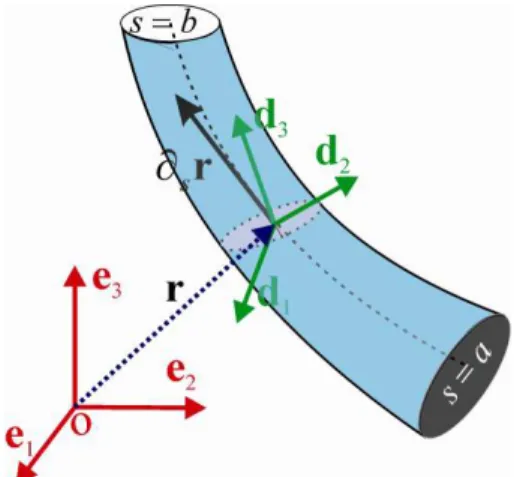
the position vector
r
( )
s t
,
expressed in terms of a fixed Cartesian basis of unit vec-torsF
=
{
e e e
1, ,
2 3}
and a set of orthogonal unity vectors attached to the moving cross section, forming the basisS
=
{
d
1( ) ( ) ( )
s t ,
,
d
2s t ,
,
d
3s t
,
}
. The variables
is the curvilinear coordinate that indicates the position of the cross section along the centroid curve, and t indicates time.Figure 1:Schematic of a Cosserat beam element.
For convenience,
d
1( )
s t
,
andd
2( )
s t
,
are assumed to be placed on the plane of the cross-section, andd
3( )
s t
,
is perpendicular to this plane. This definition implies that in the condition of pure bending, at each point of the centroid curve the direction ofd
3( )
s t
,
is coincident with the directionof the tangent to this curve, determined by
( )
s t
,
s
r
. However, when shear is accounted for, this
coincidence no longer occurs. However, it is widely accepted that, for slender beams, the shear effect can be neglected, so that the cross-sections remain perpendicular to the tangents to the centroid line (Wang et al., 2004). This assumption is adopted herein.
The motion of the centroid line
r
( )
s t
,
can be described in the inertial basis as:( )
s t
,
=
x s t
( )
,
1+
y s t
( )
,
2+
z s t
( )
,
3r
e
e
e
(1)The characterization of the motion involves both the velocity of the centroids
r
( )
s t
,
t
( )
,
( )
( )
,
,
i
i
s t
s t
s t
t
=
´
d
w
d
, i=1,2,3 (2)According to the Cosserat theory, the strains are classified in two groups: linear strains,
v
( )
s t
,
, and angular strains,u
( )
s t
,
. The components of the linear strains,v s t
1( )
,
andv s t
2( )
,
, are the shear strains, andv s t
3( )
,
is the normal strain. On the other hand, the components of angular strains,u s t
1( )
,
andu s t
2( )
,
are the bending strains, andu s t
3( )
,
is the torsion strain.The linear strain vector is given by (Wang et al., 2004):
( )
s t
,
( )
s t
,
s
=
r
v
(3)and the angular strain vector is defined in such a way that:
( )
,
( )
( )
,
,
i
i
s t
s t
s t
s
=
´
d
u
d
, i =1,2,3. (4)From Eq. (2), it follows that:
( )
1
( )
( )
,
,
,
2
i i
s t
s t
s t
t
=
´
d
w
d
(5)Similarly, from Eq. (4) one gets:
( )
1
( )
( )
,
,
,
2
i i
s t
s t
s t
s
=
´
d
u
d
(6)As stated previously, since the effect of shear is neglected, each cross-sections of the beam re-mains perpendicular to the direction defined by the tangent to the centroid curve, which enables to write:
( )
( )
( ) ( )
3,
,
,
s t
s t
,
s t
s t
s
s
=
=
r
r
v
d
(7)In this case, one has:
( )
( )
( )
( )
( )
( )
3 1 1 2 2 3 3
,
,
,
,
,
,
s t
s
s t
v s t
v s t
v s t
s t
s
=
=
+
+
r
d
e
e
e
r
(8)( )
( )
( )
1,
,
,
x s t
s
v s t
s t
s
=
r
;
( )
( )
( )
2,
,
,
y s t
s
v s t
s t
s
=
r
;
( )
( )
( )
3,
,
,
z s t
s
v s t
s t
s
=
r
(9)( )
( )
( )
2 2 2
1
,
2,
3,
1
v s t
+
v s t
+
v s t
=
(10)The cross-section rotations must be related to the linear strains in order to completely describe the kinematics of the Cosserat beam, and this can be done by using rotation parameters such as Euler angles, rotational vector (Euler vector), quaternion parameters and Cayley transformation (Dongsheng et al., 2007; Cao et al., 2008; Rubin and Brand, 2007).
In the work reported here, Euler vector and Euler angles are jointly used. First, for the parame-terization based on Euler vector, the torsion angle of the cross-section,
j
( )
s t
,
, and the linear strain vector,v
( )
s t
,
, are used as parameters. Accordingly, the following relations relating the two vector bases shown in Fig. 1 are obtained:(
)
(
)
(
)
(
)
(
)
2 2 2 2
2 3 1 3 1 2 3 1 2 1 3 2
1 2 2 2 2 1 2 2 2 2 2
1 2 1 2 1 2 1 2
1 2 3
cos
1
sin
1
cos
sin
cos
sin
v
v v
v
v v
v
v v
v
v v
v
v
v
v
v
v
v
v
v
v
j
j
j
j
j
j
é
+
-
ù
é
-
+
ù
ê
ú
ê
ú
=
ê
+
ú
+
ê
+
ú
+
ê
+
+
ú
ê
+
+
ú
ê
ú
ê
ú
ë
û
ë
û
-
-d
e
e
e
(11.a)
(
)
(
)
(
)
(
)
(
)
2 2 2 2
2 3 1 1 3 2
3 1 2 3 1 2
2 2 2 2 2 1 2 2 2 2 2
1 2 1 2 1 2 1 2
1 2 3
sin
cos
1
cos
1
sin
sin
cos
v
v v
v
v v
v
v v
v
v v
v
v
v
v
v
v
v
v
v
v
j
j
j
j
j
j
é
-
+
ù
é
+
-
ù
ê
ú
ê
ú
=
ê
-
ú
+
ê
-
ú
+
ê
+
+
ú
ê
+
+
ú
ê
ú
ê
ú
ë
û
ë
û
+
-d
e
e
e
(11.b)
3
=
v
1 1+
v
2 2+
v
3 3d
e
e
e
(11.c)Expanding Eqs. (11.a)-(11.c) in Taylor series up to the third order in terms of
v
1,v
2,j
and eliminating the termv
3with the aid of Eq. (11.c), the following relations are obtained (for simplifi-cation, time and space dependences are omitted):2 2 2 3 2
1 1 1 2 1 1 2 2 2 1 2 1 3
1
1
1
1
1
1
1
1
2
j
2
v
2
v v
j
j
2
v v
2
v
j
6
j
v
v
j
2
v
j
æ
ö
÷
æ
ö
÷
æ
ö
÷
ç
÷
ç
÷
ç
÷
» -
ç
ç
ç
-
-
÷
÷
+ -
ç
ç
ç
-
-
÷
÷
+ - -
ç
ç
ç
+
÷
÷
è
ø
è
ø
è
ø
d
e
e
e
(12.a)2 3 2 2 2
2 1 2 1 1 2 1 2 2 2 1 2 3
1
1
1
1
1
1
1
1
2
v v
2
v
6
2
2
v
2
v v
v
v
2
v
j
j
j
j
j
j
j
æ
ö
÷
æ
ö
÷
æ
ö
÷
ç
÷
ç
÷
ç
÷
» - -
ç
ç
ç
+
+
÷
÷
+ -
ç
ç
ç
-
+
÷
÷
+ - +
ç
ç
ç
+
÷
÷
è
ø
è
ø
è
ø
d
e
e
e
(12.b)( )
( )
2 23 1 1 2 2 1 2 3
1
1
1
2
2
v
v
æ
ç
v
v
ö÷
÷
»
+
+ -
ç
ç
-
÷
÷
çè
ø
After obtaining the relationship between the moving basis and the inertial basis using Euler vector, in order to relate the linear strains with angles of rotation of the cross-section, one makes use of Euler angles. Accordingly, the orientation of the moving axes is obtained by performing three successive rotations of the inertial axes. The angles of rotation about the axes
e e
1,
2and
e
3 aredefined as
f f
x,
ye
f
z, respectively.Expanding the trigonometric relations of the transformation matrix obtained through the Euler angles in third order Taylor series, and equating the resulting expression to Eqs. (12.a)-(12.c), the following relations are obtained (Cao et al., 2006):
( )
( )
2 2 21
,
1
1
( , )
( , )
( , ) ( , )
( , )
( , )
( , )
( , )
2
6
,
y x z x y z yx s t
v s t
s t
s t
s t
s t
s t
s t
s t
s t
f
f
f
f
f
f
f
¢
é
ù
=
=
+
-
ê
ë
+
+
ú
û
¢
r
(13.a)( )
( )
2 2 22
,
1
1
( , )
( , )
( , ) ( , )
( , )
( , )
( , )
( , )
2
6
,
x y z x y z xy s t
v s t
s t
s t
s t
s t
s t
s t
s t
s t
f
f
f
f
f
f
f
¢
é
ù
=
= -
+
+
ê
ë
+
+
ú
û
¢
r
(13.b)2 2
1
( , )
( , )
( , )
( , )
( , )
12
z x y z
s t
s t
s t
s t
s t
j
=
f
+
é
ê
ë
f
+
f
ù
ú
û
f
(13.c)2.2 Equations of Motion
According to Antman (1995a), from the application of the Newton-Euler equations, the local dy-namic behavior of a differential element of Cosserat beam with mass density
r
( )
s
and cross-section areA s
( )
is described by the following partial differential equations:( )
,
( )
,
( ) ( ) ( )
,
,
,
s t
s t
s t
s t
s t
t
s
=
+
´
+
h
m
v
n
l
(14.a)( ) ( ) ( )
2 2( ) ( )
,
,
,
s t
s t
s A s
s t
s
t
r
=
+
r
n
f
(14.b)where
n
( )
s t
,
,m
( )
s t
,
,h
( )
s t
,
are, respectively, the vectors of internal forces (normal and shear), internal torques (flexural and torsional) and angular momentum per unit length;f
( )
s t
,
andl
( )
s t
,
are the external force and external torque per unit length, respectively.
In order to obtain the equations of motion in terms of displacements
x s t
( )
,
,y s t
( )
,
and( )
,
z s t
, and anglesf
x( , )
s t
,f
y( , )
s t
andf
z( , )
s t
, one makes use of the relationship between the vector of angular deformationu
( )
s t
,
, and the derivatives of the directors vectorsd
1( )
s t
,
,( )
2
s t
,
d
andd
3( )
s t
,
, with respect to the spatial variables
, as expressed in Eq.(4), and the rela-tionship between the vector of angular velocityw
( )
s t
,
and the derivatives of the vectorsd
1( )
s t
,
,( )
2
s t
,
d
andd
3( )
s t
,
with respect to time, as given by Eq. (2).Thus, the derivative of the vector of internal forces with respect to s is developed as follows:
( )
3 3
1 1
1 2 3
2 3 3 2 1 3 1 1 3 2 1 2 2 1 3
i i i
i i i
i i
n
n
n
s
s
s
n
n
n
n u
n u
n u
n u
n u
n u
s
s
s
= =
é
ù
=
=
ê
+
´
ú
=
ê
ú
ê
ë
ú
û
æ
ö
÷
æ
ö
÷
æ
ö
÷
ç
÷
ç
÷
ç
÷
ç
-
+
÷
+
ç
-
+
÷
+
ç
-
+
÷
ç
÷
÷
ç
÷
÷
ç
÷
÷
ç
ç
ç
è
ø
è
ø
è
ø
å
d
å
n
d
u
d
d
d
d
(15)
Similarly, the derivatives of the vector of internal moments and angular momenta are devel-oped, respectively, as:
(
)
3 3
1 1
1 2 3
2 3 3 2 1 3 1 1 3 2 1 2 2 1 3
i i i
i i i
i i
m
m
m
s
s
s
m
m
m
m u
m u
m u
m u
m u
m u
s
s
s
= =
é
ù
ê
ú
=
=
ê
+
´
ú
=
ê
ë
ú
û
æ
ö
÷
æ
ö
÷
æ
ö
÷
ç
÷
ç
÷
ç
÷
ç
-
+
÷
+
ç
-
+
÷
+
ç
-
+
÷
ç
÷
÷
ç
÷
÷
ç
÷
÷
ç
ç
ç
è
ø
è
ø
è
ø
å
d
å
m
d
u
d
d
d
d
(16)
( )
3 3
1 1
1 2 3
2 3 3 2 1 3 1 1 3 2 1 2 2 1 3
i i i
i i i
i i
h
h
h
t
t
t
h
h
h
h
h
h
h
h
h
t
w
w
t
w
w
t
w
w
= =
é
ù
=
=
ê
+ w ´
ú
=
ê
ú
ê
ë
ú
û
æ
ö
÷
æ
ö
÷
æ
ö
÷
ç
÷
ç
÷
ç
÷
ç
-
+
÷
+
ç
-
+
÷
+
ç
-
+
÷
ç
÷
÷
ç
÷
÷
ç
÷
÷
ç
ç
ç
è
ø
è
ø
è
ø
å
d
å
h
d
d
d
d
d
(17)
Moreover, the second term on the right side of Equation (14.a) is developed as follows:
(
)
(
)
(
)
3 3
2 3 3 2 1 3 1 1 3 2 1 2 2 1 3
1 1
i i j j
i j
v
n
v n
v n
v n
v n
v n
v n
= =
æ
ö
æ
ö
÷ ç
÷
ç
÷
÷
´ =
ç
ç
÷ ç
÷
´
ç
÷
÷
=
-
+
-
+
-ç
ç
è
å
ø è
å
ø
v n
d
d
d
d
d
(18)Based on these hypotheses, the following expressions are obtained for the elements of the main diagonals of matrices
K
( )
s
andJ
( )
s
, representing the mechanical stiffness of the structure:( )
( )
( )
( )
( )
( )
11 11
,
22 22,
33 33,
J
s
= ¡
E
s
J
s
= ¡
E
s
J
s
= ¡
G
s
(19)( )
( )
( )
( )
( )
( )
11
,
22,
33K
s
=
G A s
K
s
=
G A s
K
s
=
E A s
(20)where
¡
ii( )
s
(i
=
1, 2, 3
) are the principal second moments of area of cross-section,J
11and22
J
represent the flexural rigidity,J
33 represents the torsional rigidity. The componentsK
11 and22
K
represent shear stiffness whileK
33 is the axial stiffness.Using Kirchhoff’s constitutive relations, the contact forces and moments are expressed in terms of linear and angular deformations, respectively, as follows (Cao et al., 2006):
( )
( )
( )
( )
( )
( )
( )
1 11 1
11
22 2 22 2
33 3 33 3
,
0
0
0
0
,
0
0
,
1
1
v s t
K v s
K
s
K
v s t
K v s
K
v s t
K
v s
ì
ü
ì
ü
ï
ï
é
ù ï
ï
ï
ï
ï
ï
ê
ú
ï
ï
ï
ï
ï
ï
ï
ï
ê
ú ï
ï
ï
ï
=
ê
ú ï
í
ý
ï
=
í
ï
ý
ï
ê
ú ï
ï
-
ï
ï
ï
ï
é
-
ù
ï
ï
ê
ú ï
ï
ï
ê
ú
ï
ë
û ï
î
ï
þ
ï
î
ë
û
ï
þ
n
(21)( )
( )
( )
( )
( )
( )
( )
1 11 1
11
22 2 22 2
33 3 33 3
,
,
0
0
0
0
,
,
0
0
,
,
u s t
J u s t
J
s
J
u s t
J u s t
J
u s t
J u s t
ì
ü
ì
ü
é
ù ï
ï
ï
ï
ï
ï
ï
ï
ê
ú ï
ï
ï
ï
ï
ï
ï
ï
ê
ú ï
ï
ï
ï
=
ê
ú ï
í
ý
ï
=
í
ï
ý
ï
ê
ú ï
ï
ï
ï
ï
ï
ï
ï
ê
ú ï
ï
ï
ï
ë
û ï
î
ï
þ
ï
î
ï
þ
m
(22)2.3 Finite Element Discretization
Lagrange equations are used to derive the differential equations of motion for a general Cosserat beam finite element. For this purpose, the kinetic and potential energy, as well as the virtual work of the nonconservative forces must be formulated, after performing interpolation of the displace-ment field within the eledisplace-ment.
As suggested by Cao et al. (2008), for this interpolation, non-linear shape functions obtained from the resolution of the equilibrium equations corresponding to the associated static problem are used.
This problem is represented by the following particularization of Eqs. (14.a) and (14.b):
( )
( ) ( )
0
d
s
s
s
ds
+
´
=
m
v
n
(23.a)( )
0
d
s
ds
=
n
Accounting for Eq. (18), the development of Eqs. (23.a) and (23.b) leads to the following non-linear differential equations:
( )
( ) ( )
( ) ( )
( ) ( )
( )
( ) ( )
( ) ( )
( ) ( )
( )
( ) ( )
( ) ( )
1 3 2 2 3 3 2
2 3 1 1 3 3 1
3 2 1 1 2
0
0
0
m s
u s m s
u s m s
v s n s
m s
u s m s
u s m s
v s n s
m s
u s m s
u s m s
¢
-
+
-
=
¢
+
-
+
=
¢
-
+
=
(24.a)
( )
( ) ( )
( ) ( )
( )
( ) ( )
( ) ( )
( )
( ) ( )
( ) ( )
1 3 2 2 3
2 3 1 1 2
3 2 1 1 2
0
0
0
n s
u s n s
u s n s
n s
u s n s
u s n s
n s
u s n s
u s n s
¢
-
+
=
¢
+
-
=
¢
-
+
=
(24.b)
The ordinary differential equations of static equilibrium are solved by using a perturbation technique. While the literature offers several methods, the Frobenius method (Arfken et al., 2000) was selected in this paper.
Certainly, the shape functions can be arbitrarily chosen. However, aiming at achieving the nu-merical accuracy required for representing a system undergoing large displacements, at affordable computational cost, in this paper, the shape functions were approximated using terms up to the third order, as follows:
2 3
1 2 3
( )
( )
( )
( )
( )
x s
=
x s L
=
e
x s
+
e
x s
+
e
x s
(25.a)2 3
1 2 3
( )
( )
( )
( )
( )
y s
=
y s L
=
e
y s
+
e
y s
+
e
y s
(25.b)2 3
1 2 3
( )
( )
( )
( )
( )
z s
=
z s L
= +
s
e
z s
+
e
z s
+
e
z s
(25.c)2 3
1 2 3
( )
s
( )
s L
( )
s
( )
s
( )
s
j
=
j
=
ej
+
e j
+
e j
(25.d)More details about the derivation of the shape functions using the method of perturbation can be found in Cao et al. (2008) and Wang et al. (2004).
2.4 Finite Element Dynamic Analysis
The kinetic energy per unit length of the Cosserat beam finite element is expressed as:
( ) ( ) ( )
,
( )
,
( ) ( ) ( )
1
1
,
,
2
2
T
T
s t
s t
T
s A s
s t
s
s t
t
t
r
é
ê
ù
ú
=
ê
ú
+
ê
ú
ë
û
r
r
w
I
w
(26)( ) ( ) ( )
( ) ( ) ( )
1
1
,
,
,
,
2
2
T T
U
=
ë
ê
é
v
s t
û
ú
ù
K
s
v
s t
+
ë
é
ê
u
s t
ù
ú
û
J
s
u
s t
(27)where
K
( )
s
andJ
( )
s
are defined in Eqs. (19) and (20).At the element of a single finite element, the Lagrangian function can thus be expressed in terms of a set of generalized coordinates and velocities associated to the nodal degrees of freedom,
( )e
q
andq
( )e , as follows (from now on, superscripts (e) are used to indicate quantities defined at element level):( ) ( )
(
)
( )
( )( )
( )0
,
,
,
L
e e e e
L
=
é
ê
T s
-
U s
ù
ú
ds
ê
ú
ë
û
ò
q
q
q
q
(28)while the expression of the virtual work of non-conservative forces is:
(
)
( ) ( )1 1
n N
e e
F NC
NC i i j j
i j
W
Q
q
d
d
d
= =
=
å
F
⋅
r
=
å
(29)in which NC
F
represents the resulting non-conservative forces andQ
j( )e are the generalized forces. It should be further clarified that the forces acting on the element are composed of three addi-tive parts: the first comes from the interaction between neighboring elements, i e( )f
; the second is due to the action of external concentrated forces applied at the nodes,f
c e( ); and the third is associ-ated to the loads forces distributed along the element,f
d e( ). As a result, the total virtual work done by the nonconservative forces is given by:( ) ( ) ( )
(
)
T ( )i e c e d e e F
NC
W
d
=
f
+
f
+
f
⋅
d
q
(30)Substituting Eqs. (28), (29) and (30) into the Lagrange equations, the equations of motion at element level are obtained as follows. It should be mentioned that, owing to the complexity of the algebraic manipulations involved, they have been conducted with the aid of specialized computer programs intended for symbolic manipulation:
( ) ( ) ( ) ( )
( )
( ) ( )( )
( )( )
( )( )
( )( )
( )
( )
( )
,
e e e e e i e c e d e e
e
t
+
t
+
t
=
t
+
t
+
t
M q
K q
g
q
f
f
f
q
(31)In the equation above,
M
( )e is the matrix of inertia,K
( )e is the linear stiffness matrix, and( )e
( )
( )eg
q
is the nonlinear vector containing the cubic and quadratic terms inq
( )e .global equations of motion for the system. Also, geometrical boundary conditions must be enforced by a proper modification of the global equations of motion (Bathe, 1996).
3 VISCOELASTIC FRACTIONAL DERIVATIVE MODEL
In the study reported herein, a model based on fractional derivatives was adopted for modeling of the viscoelasticity behavior in the time domain, in association with finite element discretization, according to the procedure suggested by Galucio et al. (2004).
According to the model adopted, the one-dimensional viscoelastic constitutive equation is ex-pressed as follows:
0
( )
t
aD
ta[ ( )]
t
E
( )
t
aE D
ta[ ( )],
t
s
+
t
s
=
e
+
t
¥e
(32)where
s
( )
t
is the stress,e
( )
t
is the strain,t
is the relaxation time, andE
0 andE
¥ are, respec-tively, the low-frequency and high-frequency elastic modulus. Also, in Eq. (32),D
taé ù
ê ú
⋅
ë û
indicates theRiemann-Liouville fractional derivative operator, defined as:
0
1
[ ( )]
(
)
( )d
(1
)
t td
D f t
t
f
dt
a
x
ax x
a
-=
-G -
ò
(33)where
0
< <
a
1
is the fraction derivative order andG ⋅
( )
designates the Gamma function. The fractional derivative operator is approximated by using the Grünwald-Letnikov backward-differentiation approximation, as follows:(
)
1 0
[ ( )]
(
)
,
t
N
t j
j
D f t
at
-aA
+f t
j t
=
» D
å
- D
(34)whereDt is the constant-time step used for discretization,
N
tis the number of time intervals such thatt
=
N
tD
t
, andA
j+1 are the so-called Grünwald coefficients, which are expressed as:1 1
(
)
1
,
: 1,
(
) (
1)
j
j
j
A
A
j
j
a
a
a
+
G -
-=
=
=
G - G +
(35)and satisfy the following recurrence formula:
1
1
.
j j
j
A
A
j
a
+
-=
Introducing the internal variable
( )
( )
1( )
t
t
E
t
e
e
-s
¥
which is interpreted as an anelastic strain, using the Grünwald-Letnikov approximation given in Eq. (35), and recalling that
A
1=
1,
one obtains:(
)
1 0 1 1
1 1
1
t
N
n n n j
j j
E
E
c
c
A
E
e
+ ¥e
+e
+-+ = ¥
-=
-
-
å
(37)where
c
t
a a at
t
=
D +
and the notation(
)
n
f n t
D =
f
has been introduced.Associating Eqs. (32) and (37), the following discretized form of the constitutive equation is ob-tained:
1 0 1 1
0 1 1 0 0
1
t Nn n n j
j j
E
E
E
E
c
c
A
E
E
s
+ ¥e
+ ¥e
+-+ =
æ
-
ö
÷
ç
÷
ç
=
ç
+
÷
÷÷
+
çè
ø
å
(38)The discrete-time constitutive equation applicable to multiaxial stress/strain states can be ob-tained by replacing the scalar stress, strain and material moduli by the respective equivalent vectors and matrices, as follows:
1 0 1 1
0 1 1 0 0
1
t Nn n n j
j j
E
E
E
E
c
c
A
E
E
+ ¥ + ¥ +
-+ =
æ
-
ö
÷
ç
÷
ç
=
ç
+
÷
+
÷÷
çè
ø
å
(39)In the derivation of Eq. (39), it has been assumed that:
(
0)
(
)
0
;
2 1
2 1
E
E
G
G
n
n
¥ ¥=
=
+
+
(40)in such a way that the material coefficient matrices can be expressed as:
0
=
E
0
;
¥=
E
¥
E
E E
E
(41)where matrix
E
depends only on the Poisson ratio .One way to include the viscoelastic behavior into the finite element model is by formulating the virtual work done by the non-conservative internal forces developed within a viscoelastic material. For this purpose, one resumes the development presented in the previous section, writing:
( )
( ) ( ) T ( ) ( )
[
( , )]
( , )d
e
e e e e
i V
W
s t
s t
V
d
= -
ò
s
d
e
(42)Considering the viscoelastic fractional derivative model, ( )e
( , )
s t
s
may be obtained from Eq. (39)in the following form:
σ
( ) 1ε
( ) 1 ( )ε
( )0 0 0 0 1 1 0
( , )
[1
(
)]
( , )
NP( ,
),
e e e e
j j
s t
c E
-E
¥E
s t
c E E
- ¥A
+a
s t
j t
=
and the virtual work of the internal forces is obtained as follows:
( )
( ) ( ) T ( ) ( )
T
1 ( ) ( ) 1 ( ) ( ) ( )
0 0 COS 0 1 1 COS
[
( , )]
( , )d
[1
(
)]
(
)
(
)
( ),
e
P
e e e e
i V
N
e e e e e
j t j t j
W
s t
s t V
cE
E
E
cE E
A
t
d
d
a
d
-
-¥ ¥ = + - D
=-
s
e
é
ù
=- +
ê
-
+
ú
ë
û
ò
å
F
q
F
q
q
(44)where:
( ) ( ) ( ) ( ) ( ) ( )
COS
(
)
(
)
[
(
)]
e e e e e e
t j t- D
=
t
- D +
j t
t
- D
j t
F
q
K q
g
q
(45)and,
( ) 1 ( ) ( )
0 1 1
( )
(1
)
(
)
( )
NP(
).
e e e
j j
t
c E
¥-E
¥E
t
c
A
+a
t
j t
=
= -
-
-
å
- D
q
q
q
(46)Noting that the inclusion of the viscoelastic behavior does not affect the kinetic energy, upon using the Lagrange Equations, the following nonlinear differential equations of motion for a Cosse-rat viscoelastic beam at elementary level are obtained:
( ) ( ) 1 ( ) ( ) ( ) ( )
0 0
( ) ( ) ( ) ( ) 1 ( ) ( )
0 1 1 COS
( )
[1
(
) ]
( )
(
)
( )
( )
( ,
)
P(
).
e e e e e e
N
i e c e d e e e e
j t j t j
t
c E
E
E
t
t
t
t
cE E
A
a
-¥
-¥ = + - D
é
ù
+ +
-
ê
ë
+
ú
û
=
=
+
+
-
å
M
q
K q
g
q
f
f
f
q
F
q
(47)
Regarding the numerical resolution of the global equations of motion, a composite, implicit time integration scheme, previously proposed by Bathe and Baig (2005), has been chosen, since it has been found to provide accurate results with a constant time step. This latter is a constraint imposed by the Grünwald-Letnikov scheme adopted for the discretization fractional derivatives. Therefore, the numerical algorithm implemented consists in computing an intermediate response between time instants
t
andt
+ D
t
based on the trapezoidal rule, and using backward-differentiation formulae to evaluate the response att
+ D
t
, from the response calculated at instantt
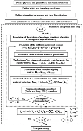
and the intermediate response. Clearly, since the method is implicit, a method intended for solving nonlinear algebraic equations, such as Newton-Raphson, has also been used.The flowchart presented in Fig. 2 illustrates the main operations involved in the computation of time domain responses associating Cosserat beam theory and fractional derivative model.
4 NUMERICAL SIMULATIONS
Figure 2: Procedural flowchart for the computation of time domain responses associating Cosserat beam theory and fractional derivative model.
Figure 3: Structures considered in the numerical simulations: (a) clamped-free beam subjected to axial load; and (b) clamped-free beam subjected to transversal load,
(c) Time variation of the external loads applied to cases (a) and (b).
b h
F(t) L
x y
z (a)
F(t) h
L b
x y
z (b)
F
(
t
) [N]
t [s] F0
4.1 Axial Loading
For the axial loading case, the dimensions of the beam illustrated in Fig.3(a), are as follows: L=500 mm, b=50 mm, h=50 mm. This example was considered by Galucio et al. (2004). Although it does not involve transverse motion, it is considered to be useful for validation of the numerical imple-mentation of the Cosserat theory in association with the viscoelastic model, by comparison with results available in the literature. The properties adopted for the viscoelastic material are: r=1000 kg/m3,
E
0= 7 MPa,E
¥= 10 MPa,t
= 20 ms anda
= 0.5. The external load is applied at the free-end of the clamped beam, acting along the positive direction of the longitudinal x axis, as illus-trated in Fig. 3(a). According to Fig. 3(c) this load is given byF t
( )
=
F H t
0( )
, withF
0=
1 N, beingH t
( )
the unit-step function (Heaviside function).Spatial discretization is done with 10 finite elements, leading to a mesh with 11 nodes and 66 degrees of freedom before the enforcement of the boundary conditions. Total simulation time has been chosen as 400 ms, and integration was performed with a time increment of 1 ms.
Figure 4 shows the normalized axial displacement of the tip of the viscoelastic beam, calculated through the Cosserat/fractional derivative modeling approach, as compared to other modeling strategies. These latter are based on a three-layer sandwich beam finite element, containing a visco-elastic core between two visco-elastic faces, developed by Galucio et al. (2004). This model degenerates to a Timoshenko beam element when the outer faces are neglected.
Figure 4: Normalized axial displacement of the tip of the viscoelastic beam shown in Fig. 3(a).
4.2 Transverse Loading
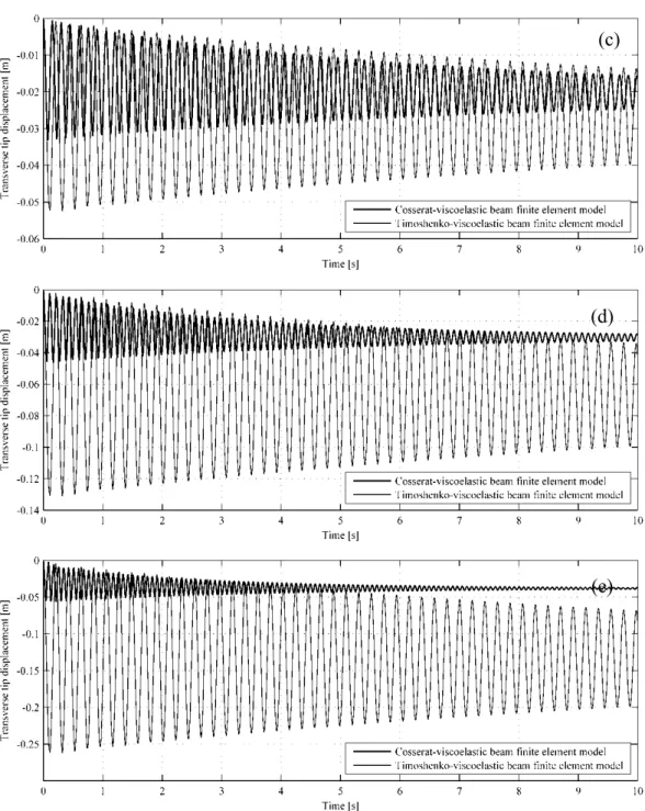
The transverse-loaded slender beam considered in Fig. 3(b) is now addressed. The beam dimensions are L=500 mm, b=50 mm, h=50 mm. The viscoelastic material parameters are: r=1000 kg/m3,
0
E
=2.98 GPa,E
¥=
3.18 GPa,t
= 63.16 ms anda
= 0.35.The transverse load, expressed as
F t
( )
=
F H t
0( )
, is applied at the free-end of the clamped beam, as shown in Fig. 3(b), and takes, successfully, the following values of amplitude: 0.01 N, 0.5 N, 1 N, 2.5 N and 5 N. This pattern has been chosen to demonstrate increasing nonlinear behavior with increasing load. The discretization mesh employed in this case consists of 20 elements, 21 nodes, and 126 degrees of freedom (before enforcing boundary conditions). A simulation time of 10s was adopted, and numerical integration was performed with a time increment of 2 ms.In Fig. 5 the results, in terms of transverse displacement at the free end of the beam, are com-pared to counterparts obtained from a linear viscoelastic beam finite element model based on Timo-shenko beam theory, also implemented by the authors.
It can be clearly seen that as the magnitude of the load increases, thus inducing increasing geo-metric nonlinearities, the response predicted by the linear Timoshenko beam theory and the nonlin-earCosserat beam theory progressively deviate from each other. Differences are observed not only in the vibration frequency and amplitude but also in the damping level.
(a)
Figure 5: Transverse displacement of the free-end of the beam shown in Fig. 4.1(b) for different loading intensities: (a)
F
0= 0.01 N; (b)F
0=0.5 N; (c)F
0=1.0 N; (d)F
0=2.5 N; (e)F
0=5 N.5 CONCLUSIONS
This paper proposed a modeling strategy for viscoelastic slender structures consisting in the associa-tion of the nonlinear Cosserat beam theory with a fracassocia-tional differential viscoelastic model. The