A Work Project, presented as part of the requirements for the Award of a Masters Degree in Finance from the NOVA – School of Business and Economics.
Financial Depth, Stock Markets and Economic Growth in the EU-15 countries
Ana Sofia Falcão Félix de Almeida, nº762
A Project carried out on the Finance course, under the supervision of:
Luciano Amaral
2
Financial Depth, Stock Markets and Economic Growth in the EU-15 countries
Author: Ana Sofia Almeida
Supervisor: Luciano Amaral
7th January 2015
ABSTRACT
The aim of this paper is to assess the impact of financial depth on economic growth in the EU-15 countries from 1970 until 2012, using the two-step System GMM estimator. Even though it might be expected a positive impact, the results show it is negative and sometimes even negative and statistically significant. Among the reasons presented for this, the existence of banking crises seems to better explain these results. In tranquil periods, financial deepening appears to have a positive impact, whereas in banking crises it is persistently negative and statistically significant. Also, after an assessment of the impact of stock markets on economic growth, it appears that more developed countries in the EU-15 have an economy more reliant on this segment of the financial system rather than in bank intermediation.
3 I. Introduction
King and Levine argued in their paper in 1993 that financial depth does not only
influence economies’ efficiency and investment rates, but it also has a crucial role in
fostering economic growth (King and Levine, 1993). The main idea behind this reasoning is that finance can theoretically mitigate the effects of information and transaction costs, solving potential market frictions. Therefore, financial systems may influence investment decisions, technological innovation and saving rates, which in turn can influence long-run growth rates. However, in real conditions, authors seem to struggle to fully comprehend the complex and intricate relationship between the financial system and growth. There have been many hypothesis related to the finance-growth nexus.
4 Although there seems to be a contradiction upon the degree and role of finance in economy, many authors noticed the apparent lack of importance of financial depth in growth, especially when considering the latest years. So, this paper follows some of the most plausible reasons stated by authors in this field and also checks other factors characteristic of the EU-15. In order to perform this analysis, a series of tests were made, using various measures of financial deepening, namely Domestic Credit, Private Credit and Liquid Liabilities as percentage of GDP in the EU-15 countries, covering the period from 1970 until 2012, together with diverse control variables typical of growth regressions. In order to better control for endogeneity and small sample problems the System GMM two-step estimator was used, as first proposed by Arellano and Bover (1995) and later by Blundell and Bond (1998).
5 II. Literature Review
The importance of the financial system has been thoroughly discussed by several economists. Hypothetically, it can have a significant influence mitigating the effects of information and transaction costs, which can influence investment decisions, long-run growth rates, technological innovation and saving rates. However, not every economist agrees upon the degree of impact that the financial system can have on economic growth and the results of empirical studies in this area have been rather inconclusive. Some authors have been able to find strong evidence to support the importance of the financial system for economic growth, but others have only found weak or mixed evidence.
According to King and Levine’s results (1993) the improvement in the rates of capital accumulation and the increase of economies’ efficiency in employing capital can be explained by higher levels of financial development. Thus, they were able to show evidence that finance does not only follow economic activity, as stated by Joan Robinson (1952), but that it is also a critical part of the growth process. Since then, many other authors were able to show the crucial role played by the financial system in fostering economic growth by facilitating resource allocation and fostering productivity growth (e.g. Beck, Levine and Loayza, 2000). Regarding financial markets, Atje and Jovanovic (1993) were able to show a positive impact on economic growth, while
6 Nonetheless, some authors do not think that the positive relationship between finance and growth is clear and that it can be rather complex or even non-existent. Robert Lucas (1988), for example, believes that the role of financial factors is overstated when explaining economic growth. On the other hand, there is evidence showing that financial development has a stronger positive impact in middle-income countries, but it tends to decrease as they become richer (Rioja and Valev, 2004a, 2004b, and Aghion, Howitt and Mayer-Foulkes, 2005). In a more recent study made by Arcand, Berkes and Panizza (2012), the results show evidence of a turning point of approximately 100 percent private credit to GDP, where the finance-growth relationship becomes negative. The reasons given by these authors to explain these results were banking crises, economic volatility and the way through which finance is provided, among others. Furthermore, according to the results from the Rousseau and Watchel’s study (2011), the effect of financial deepening was stronger between the 1960s and 1980s, but tended to disappear throughout the subsequent years. One of the reasons proposed to explain this fact was the instability and the complexity of the finance-growth relationship. Also, the excessive financial deepening and the too rapid credit growth may lead to inflation and the weakening of banking systems, which in turn may lead to financial crises. In these turbulent periods the benefits of financial depth in economic growth would disappear.
7 III. Data and Methodology
In order to analyze the effect of financial depth on economic growth, the dependent variable used was the growth rate of real GDP per capita, retrieved from the World Bank’s World Development Indicators (WDI). As indicators of financial depth, Private Credit by Financial Sector (PC), Domestic Credit by Financial Sector (DC) and Liquid Liquidities (LiqLiab) were used, all in percentage of GDP. The data for these three variables were also retrieved from the World Bank’s WDI. Furthermore, all regressions included, as control variables, the log of initial GDP per capita (GDP initial), the percentage of secondary education attainment (Educ), the sum of exports and imports of goods and services as percentage of GDP (Trade), the ratio of government expenditures to GDP (GovExp) and the inflation rate (Inf). These control variables were retrieved from the WDI database, except for the percentage of the secondary education attainment which came from the Barro and Lee database.1
The panel consists of data from the EU-15 countries, namely Austria, Belgium, Denmark, Finland, France, Germany, Greece, Ireland, Italy, Luxembourg, Netherlands, Portugal, Spain, Sweden and United Kingdom, over the period from 1970 until 2012. The data is averaged in eleven non-overlapping 4-year periods, except for the last period that results from the average of the last three years. This procedure is used to better analyze the medium-term relationship between finance and growth, and control for the instability of the business cycle.2
1 The Barro and Lee’s database covered data in 5-year time-span. For this paper, I estimated the missing
values by admitting a linear relationship between the existing values. Afterwards, they were imputed in averages in 4-year periods.
2 Even though it will result in fewer observations per variable, this procedure was recommended when
8 In this study, the GMM system estimator was used, as proposed by Arellano and Bover (1995) and Blundell and Bond (1997). Also, all regressions will adopt the two-step procedure and obtain robust standard errors using the Windmeijer (2005) finite sample correction, which helps to solve the problem of downward biased standard errors common in the two-step procedure. Thus, it will provide more asymptotic efficient estimates than the one-step procedure.
There are several reasons behind the choice of this dynamic panel regression. First, this method helps to solve endogeneity problems, which are rather frequent in the analysis of economic growth. By using lagged values of the endogenous variables as internal instruments, more accurate conclusions can be drawn. Second, the system GMM is appropriate for small T periods, which in this case are just eleven. Finally, the system estimator is expected to reduce potential biases in finite samples and asymptotic imprecision which is common in the difference GMM estimator.
All regressions included control variables, namely Education, Government Expenditure, Trade, Inflation and the logarithm of initial real GDP per capita. Also, the instruments used were the lags of these same variables, as well as the main explanatory variable and the time fixed effects.3
Section IV will detail an analysis of the results for the System GMM estimations for each measure of finance depth. Afterwards, in Section V there will be a further analysis in order to assess what factors can impact either positively or negatively the finance-growth nexus. Finally, in Section VI, we turn our attention towards the impact
3 The numbers of lags imputed were two in order to avoid the problem of “too many instruments”, since
9 of stock markets in economic growth, using as variables the Market Capitalization as percentage of GDP and the Volume of Stock Traded to GDP. However, in this latter analysis, the data covers only the period from 1989 until 2012 due to lack of data availability. This analysis of the stock market provides an additional perspective to assessing financial depth and the role of the financial system in economic growth.
IV. The impact of financial depth
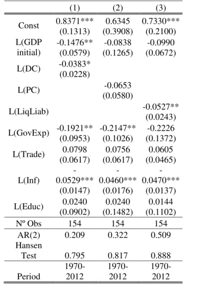
Having established the methodology and procedure used, the first regressions to be made are represented in Table I. Each column corresponds to a regression made for each measure of financial depth. According to the results, the three measures of financial depth do not have a positive and significant impact in economic growth in the EU-15 countries. In fact, they are persistently negative and sometimes even statistically significant.
Starting with Domestic Credit provided by Financial Sector [L(DC)], it shows a negative impact in economic growth of 0.038 with a statistical significance of 10%. Moving on to Private Credit provided by Financial Sector [L(PC)], its coefficient shows that it has a negative impact of 0.065 in economic growth. Finally, Liquid Liabilities [L(LiqLiab)] have an impact equal to -0.053 with a statistical significance of 5% in economic growth.
10 V. Discussion of the results
Even though the results from Table I report a lack of positive benefits of financial depth in the economic growth, this same relationship can be complex and other aspects may influence these same results. Thus, a further analysis was performed, adding new control variables that could have a crucial impact and change the results stated in Table I.
V.I. Banking Crisis
First, the most plausible reason why financial depth may display a negative impact in economic growth is the existence of banking crises. As stated by Rousseau and Wachtel (2011), a rapid credit growth can lead to financial and banking crises, thus
provoking the “vanishing effect” in financial depth upon the economic growth.
Therefore, a dummy variable was added representing the existence of banking crisis (BKCR) in this sensitivity analysis. In particular, BKCR is equal to 1 in periods that signal the presence of a banking crisis and 0 in tranquil periods.4 The regressions in column (2) in Table II, III and IV show the coefficient of each measure of financial depth and then the finance variable when interacted with this dummy.5 According to the results, the coefficients of Domestic Credit and Private Credit are larger and became positive in tranquil periods, even though they are not statistically significant. As for Liquid Liabilities in Table IV column (2), the coefficient remains negative but loses its significance. Regarding the interaction between finance and banking crises, this variable
4 Data retrieved from Carmen M. Reinhart and Kenneth S. Rogoff (2010)
5 When multiplying the banking crisis dummy with the financial depth measure, the respective
coefficient given represents the importance of financial deepening in these turbulent periods.
11 shows the difference in the finance effect when a country is in crisis. In every case, the corresponding coefficient is smaller, statistically significant at 1 percent level and approximately equal to -0.011. Thus, when a country is facing a banking crisis, the finance effect is likely to disappear and becomes negative. On the other hand, when facing a tranquil period the finance-growth relationship seems to become positive. However, the positive coefficient of finance in column (2) in Table II and III is not statistically significant, meaning that there could be other possible factors to explain this dynamic between finance and growth.
V.II. Euro and PIIGS
In order to check whether national peculiarities within the European Union can have an impact in the financial depth coefficient, the two variables chosen were the dummies PIIGS and Euro6. The first is used to see the difference when just analyzing the PIIGS countries, namely Portugal, Ireland, Italy, Greece and Spain. These five countries of southern Europe have similar economic environments and have a history of facing high unemployment, economic difficulties and political instability. Due to these difficulties, it is expected that the financial deepening has a higher impact in these countries, since they have to resort to finance in order to overcome them, leaving these countries with their characteristic high debt burden. Afterwards, by analyzing the role of the introduction of the Euro currency, it is expected that, by improving financial integration, it would result in a higher impact on financial depth and therefore in economic growth.
6 Euro dummy is equal to 1 after the introduction of the Euro currency and 0 before that. The PIIGS
12 According to the results from Table II to Table IV in column (3) and (4), when controlling for the dummies PIIGS and Euro, the coefficient that demonstrates the interaction between these variables and finance became higher than the coefficient of the measures of financial depth. In the PIIGS countries financial depth has an impact ranging between -0.002 and -0.014, becoming statistically significant only at 10% level in Liquid Liabilities. Regarding non-PIIGS countries, the impact on finance is even more negative, except from Liquid Liabilities. As for the introduction of the Euro, the impact of finance ranges from -0.006 and -0.008, becoming statistically significant only at 10% level in Domestic Credit. This indicates that financial depth has a higher impact in economic growth in the PIIGS countries and also after the introduction of the Euro. However, it still reports a negative coefficient, so, even though they have a less negative impact, financial deepening still appears not to be a positive factor in economic growth.
V.III. Political Instability and Government Quality
When faced with the uncertainty associated with an unstable political environment, investment tends to decrease, as well as economic development, since
investor’s confidence upon the success of the country is shaken. It might be difficult to analyze this relationship since poor economic growth may cause changes in government and citizens may believe that by changing the government their situation might improve. In order to analyze the role of political instability a dummy variable was introduced, where it is equal to one when the government changes7. The objective is to see if this variable might help explain the negative and significant coefficient of financial depth. According to the results from Table II, III and IV in column (5), the
7 Own elaborations based upon the database of Armingeon, Knöpfel, Weisstanner, Engler, Potolidis and
13 dummy is negative but not statistically significant, ranging from -0.001 to -0.005. Also, by adding this dummy the coefficients of financial depth lose their significance, but still remain negative.
According to Demetriades and Law (2006), financial depth loses its positive impact in economic growth in countries with poor institutions and low quality governments. Therefore, in this study it is added a time-invariant variable “Low
GovQual”, based on a quality government index ranging from 0 to 10, which is equal to 1 if the government quality index is below 7.5, 0.5 if it is between 7.5 and 9.0 and 0 if it is above 9.0.8 The results from Table II in column (6) show that when analyzing the interaction between Domestic Credit and the low government quality, its coefficient is lower, but insignificant, which can entail that poor quality government does indeed translate into a lower impact of finance in economy. However, in Table III and IV in column (6), this same coefficient has a higher coefficient than the finance variable itself. Therefore, Domestic Credit in countries with poor government quality has an even more negative impact in economic growth, but this does not occur on Private Credit and Liquid Liabilities, where poor government seems to have a positive impact in this finance-growth relationship. Even though this might seem strange, the interaction term only has statistical significance when dealing with Liquid Liabilities. Thus, since the results can be rather contradictory and two of them do not have significance, no proper conclusions can be reached upon the influence of poor government quality.
8 Database from QOG Institute of the University of Gothenburg and it results from the mean value of
14 V.IV. Credit Regulation, Stock Market Liberalization and Economic Freedom
In finance, credit regulation can have a crucial role in influencing the economic growth of a country. Even though credit regulation is normally tight in order to prevent crises and limit the amount of systemic risk, this can result on a lower financial development and, therefore, lower growth. In order to analyze the importance of credit constraints, a time-invariant variable will be added “Credit Constraints” based upon an index of Credit Regulation ranging from 0 to 10.9 This variable will be equal to 1 if this index is lower than 5, 0.5 if it is between 5 and 7.5, and 0 if it is above 7.5. The results from Table II, III and IV in column (7) show that the coefficient of the interaction between credit constraints and finance is higher than the variable of finance itself. This may be due to the efficiency in which credit is regulated, since there is a similarity in regulation of credit amongst the EU-15, especially after the introduction of Basel II. However, the interaction term is not statistically significant and it is still negative, so no concrete conclusions can be obtained.
The disappearance of the finance effect in growth can also be explained by the rapid liberalization of stock markets in the latter period, since stock markets may have acted as a substitute for credit market financing. However, it might be difficult to study the importance of liberalization in the finance-growth relationship, since liberalization
itself can be a great contributor to economic growth. The dummy variable “SMLib”
introduced in the regressions in Table II through IV in column (8) will be equal to 1
9 Data based upon the Economic Freedom of the World Index. The index is based upon the extent to
15 when the country began to have a fully liberalized equity market.10 According to the results, the coefficient that demonstrates the interaction between finance and liberalization of equity market is always positive and statistically significant when it comes to Domestic Credit and Liquid Liabilities. Thus, the finance effect is in fact stronger after liberalization of stock markets. However, as stated before it can be difficult to ascertain exactly what the impact of this dummy can be on the finance-growth relationship and most of the more developed countries already had a fully liberalized stock market since 1970. So, the effect before and after this equity market opening can’t be properly analyzed, but it indicates that the liberalization of equity markets may not have the negative impact in the finance-growth nexus that it might have been expected.
Finally, the time-invariant variable “EFW” was added in order to assess whether the overall freedom of a country could influence the finance-growth nexus and also if other factors, rather than stock market liberalization and credit regulation, may have an impact. This variable was derived from the Economic Freedom of the World index ranging from 0 to 10, assuming the value 0 if the index is below 5, 0.5 if it is between 5 and 7.5, and 1 if it is above 7.5. According to the results from Table II, III and IV in column (9), this variable presents always a positive coefficient, but not statistically significant. Also, the coefficient of Liquid Liabilities remains negative and statistically significant by 10% level. Concerning Domestic Credit, it remains negative but loses its significance, whereas the Private Credit remains negative but now is statistically significant at 10% level. Thus, the overall economic freedom does not appear to a have a significant impact on economic growth.
16 VI. Stock Markets
As countries become more developed it is expected that they rely more on the development of stock market and use it as a substitute for credit market financing. Therefore, since all EU-15 countries are developed and have a fully liberalized equity market for a relatively large period of time, an analysis was made in order to assess whether this specific segment of the financial system can have a more significant contribution to growth than bank intermediation. Thus, the variables Stocks Traded as percentage of GDP and the Market Capitalization as percentage of GDP will be used to test this hypothesis.11
According to the results presented in Table V in column (1) the market capitalization shows a positive impact on economic growth of 0.061 with a statistically significance of 1% level. On the other hand, the coefficient of stocks traded in column (4) show a positive value of 0.016 but do not have any significance. By analyzing both variables considering the interaction term with the Stock Market Crisis dummy variable, the coefficient of the main variables remain the same, but in this case the market capitalization has only 5% significance level.12 Also, the interaction term shows that, in periods of crises, the impact of stock market in economic growth is negative, even though it is not statistically significant.
Finally, the interaction between equity markets and the PIIGS countries is analyzed in columns (3) and (6) in Table V. According to the results, the volume of Stocks Traded has a more significant impact in growth in non-PIIGS countries, being
11 The data covers the period from 1989 until 2012 and is averaged in six non-overlapping 4-year
periods. The method used will still be the system GMM estimator with the two-step procedure with robust standard errors using the Windmeijer (2005) finite sample correction. The data of Market Capitalization and Volume of Stocks Traded was retrieved from the WDI database.
17 equal to 0.024 with a statistical significance of 1% level. Meanwhile in Portugal, Ireland, Italy, Greece and Spain, the volume of Stocks Traded is -0.016 with a significance level of 5%. Also, the coefficient of Market Capitalization in PIIGS countries is -0.016, but is not statistically significant. Regarding the Market Capitalization in non-PIIGS countries, its coefficient remains positive with a significance level of 5% and equal to 0.065. Therefore, in PIIGS countries the stock market may not be as well developed as in other countries in the EU-15. Also, since in these countries the effect of finance is slightly larger, maybe they have not made the complete transition towards a more developed economic model, more reliant on stock markets.
VII. Conclusion
This paper examines the impact of financial depth on economic growth in EU-15 by using the dynamic panel techniques proposed by Arellano and Bover (1995), and Blundell and Bond (1997). As stated in previous sections, financial deepening does not appear to have a positive impact in economic growth in these fifteen countries. Alternatively, possible reasons for this apparently negative relationship were examined.
Firstly, the most plausible reason is the existence of banking crises during the time period from 1970 until 2012. It seems that financial depth has a positive impact on economic growth in tranquil periods, but it disappears as countries face a crisis. This same conclusion was also reached by Rousseau and Watchel (2011), who also defend that excessive deepening may actually be responsible for banking and financial crises.
18 even though less developed countries seem to rely more upon the financial development, this is still not positive and significant. The same happens with the introduction of the Euro. So, these two factors did not have a great influence on the negative finance-growth relationship.
Thirdly, government changes do not appear to change the results stated in Table I and do not have a significant negative impact on economic growth. On the other hand, poor quality governments may have an effect on finance, but just when analyzing Domestic Credit. It would seem that in poor quality governments the impact of Domestic Credit on economic growth is even more negative. However, these same results do not stand for Private Credit and Liquid Liabilities. Finally, credit regulation, stock market liberalization and economic freedom still do not change the negative correlation between finance and growth. However, there might be other possible reasons and factors, namely bank efficiency, which could have a positive and significant influence in economic growth and, as banks become more efficient, the financial deepening has a greater and more effective impact upon economic growth.
19 References
Aghion, Philippe, Peter Howitt, and David Mayer-Foulkes. 2005. "The Effect of Financial Development on Convergence: Theory and Evidence," The Quarterly Journal of Economics, MIT Press, vol. 120(1): 173-222.
Arcand, Jean-Louis, Enrico Berkes, and Ugo Panizza. 2012. “Too Much Finance?” IMF Working Papers 12/161, International Monetary Fund.
Arellano, Manuel, and Olympia Bover. 1995. “Another look at the instrumental variables estimation of error-components models.” Journal of Econometrics, 68(1): 29-51.
Armingeon, Klaus, Laura Knöpfel, David Weisstanner, Sarah Engler, Panajotis Potolidis, and Marlène Gerber. 2013. “Comparative Political Data Set I 1960-2011.” Bern: Institute of Political Science, University of Bern.
Atje, Raymond, and Boyan Jovanovic. 1993. “Stock Market and Development.”
European Economic Review, 37: 632-640.
Baum, Christopher F., Schaffer, Mark E., and Stillman, Steven. 2003. “Intrumental Variables and GMM: Estimation and Testing”. The Stata Journal, 3: 1-31.
Beck, Thorsten, Ross Levine, and Norman Loayza. 2000. “Finance and the Sources of
Growth.” Journal of Financial Economics, 58: 261-300.
Bekaert, Geert, Campbell R. Harvey, and Christian Lundblad. 2005. “Does Financial Liberalization Spur Growth?” Journal of Financial Economics, 77: 3-55.
Blundell, Richard, and Stephen Bond. 1998. “Initial conditions and moment restrictions
in dynamic panel data models.” Journal of Econometrics. 87(1): 115-143.
Demetriades, Panicos O., and Siong Hook Law, (2006). "Finance, institutions and economic development." International Journal of Finance and Economics, 11(3): 245-260.
King, Robert G., and Ross Levine. 1993. “Finance and Growth: Schumpeter Might Be
20 Levine, Ross, and Sara Zervos. 1998. “Stock Markets, Banks and Economic Growth.”
American Economic Review, 88: 537-558.
Lucas, Robert. 1988. “On the Mechanics of Economic Development.” Journal of Monetary Economics, 22(1): 3-42.
Rajan, Raghuram, and Luigi Zingales. 1998. “Financial Dependence and Growth.”
American Economic Review, 88: 559-586.
Reinhart, Camen M. and Kenneth S. Rogoff. 2010. “From Financial Crash to Debt Crisis.” American Economic Review, 101(5): 1676-1706.
Rioja, Felix, and Neven Valev. 2004a. “Finance and Sources of Growth at Various
Stages of Economic Development.” Economic Inquiry, 42: 127-140.
Rioja, Felix, and Neven Valev. 2004b. “Does One Size Fit All? A Reexamination of the
Finance and Growth Relationship.” Journal of Development Economics, 74: 429-447.
Robinson, Joan. 1952. “The Generalization of the General Theory.” The rate of interest, and other essays. London: Macmillan: 67-142.
Roodman, David. 2006. “How to do xtabond2: An Introduction to “Difference” and “System” GMM in Stata”. Center for Global Development: 1-44.
Rousseau, Peter, and Paul Watchel. 2011. “What is Happening to the Impact of Financial Deepening on Economic Growth?” Economic Inquiry, 49: 276-288.
21 Appendix
Table I – System GMM estimations for Domestic Credit (DC), Private Credit (PC) and Liquid Liabilities (LiqLiab)
System GMM estimations of 4-year non-overlapping growth spells from 1970 until 2012, using as instruments the lags of financial depth measures, Initial GDP, Trade, Government Expenditure (GovExp), Inflation (Inf) and Education (Educ) in form of logarithms, as well as time fixed effects. The control variables used were: log of Initial GDP, log of Education, log of Trade, log of Government Expenditure and log of Inflation.
(1) (2) (3)
Const 0.8371*** 0.6345 0.7330*** (0.1313) (0.3908) (0.2100) L(GDP
initial)
-0.1476** -0.0838 -0.0990 (0.0579) (0.1265) (0.0672) L(DC) -0.0383*
(0.0228)
L(PC) -0.0653
(0.0580)
L(LiqLiab) -0.0527**
(0.0243) L(GovExp) -0.1921** -0.2147** -0.2226
(0.0953) (0.1026) (0.1372) L(Trade) 0.0798 0.0756 0.0605
(0.0617) (0.0617) (0.0465) L(Inf) -0.0529*** -0.0460*** -0.0470*** (0.0147) (0.0176) (0.0137) L(Educ) 0.0240 0.0240 0.0144
(0.0902) (0.1482) (0.1102)
Nº Obs 154 154 154
AR(2) 0.209 0.322 0.509
Hansen
Test 0.795 0.817 0.888
Period 1970-2012 1970-2012 1970-2012
22 Table II – Sensitivity Analysis of Domestic Credit
System GMM estimations of 4-year non-overlapping growth spells from 1970 until 2012, using as instruments the lags of Domestic Credit (DC), Initial GDP, Trade, Government Expenditure (GovExp), Inflation (Inf) and Education (Educ) in form of logarithms, as well as time fixed effects. The control variables (log of Initial GDP, log of Education, log of Trade, log of Government Expenditure and log of Inflation) were omitted due to a matter of space. The remaining control variables are reported in this Table and are added one by one.
(1) (2) (3) (4) (5) (6) (7) (8) (9)
L(DC) -0.038* 0.038 -0.065 -0.065** -0.060 -0.041 -0.047 -0.056 -0.044 (0.023) (0.031) (0.032) (0.037) (0.052) (0.067) (0.034) (0.037) (0.043)
BKCR*L(DC) -0.011***
(0.006)
PIIGS*L(DC) -0.008
(0.019)
Euro*L(DC) -0.008*
(0.010)
Changes in Gov -0.005
(0.015) Low
GovQual*L(DC)
-0.072 (0.173) Credit
Constraints* L(DC)
-0.012
(0.011) SMLib
*L(DC)
0.014* (0.008)
EFW 0.042
(0.067)
Nº Obs 154 154 154 154 154 154 154 154 154
AR(2) 0.209 0.276 0.324 0.106 0.252 0.192 0.765 0.160 0.083
Hansen Test 0.795 0.991 0.934 0.767 0.865 0.818 0.720 0.792 0.878
23 Table III – Sensitivity Analysis of Private Credit
System GMM estimations of 4-year non-overlapping growth spells from 1970 until 2012, using as instruments the lags of Private Credit, Initial GDP, Trade, Government Expenditure, Inflation and Education in form of logarithms, as well as time fixed effects. The control variables (log of Initial GDP, log of Education, log of Trade, log of Government Expenditure and log of Inflation) were omitted due to a matter of space. The remaining control variables are reported in this Table and are added one by one.
(1) (2) (3) (4) (5) (6) (7) (8) (9)
L(PC) -0.065 0.027 -0.094* -0.066 -0.056 -0.065 -0.068 -0.068 -0.068* (0.058) (0.040) (0.053) (0.067) (0.058) (0.047) (0.045) (0.059) (0.040)
BKCR*L(PC) -0.011***
(0.005)
PIIGS*L(PC) -0.002
(0.013)
Euro*L(PC) -0.006
(0.010) Changes in
Gov
-0.001 (0.014) Low
GovQual* L(PC)
-0.006
(0.010)
Credit Constraints
*L(PC)
-0.006
(0.016)
SMLib
*L(PC) 0.011
(0.010)
EFW 0.046
(0.052)
Nº Obs 154 154 154 154 154 154 154 154 154
AR(2) 0.322 0.655 0.323 0.259 0.370 0.347 0.663 0.405 0.170
Hansen Test 0.817 0.996 0.877 0.782 0.783 0.855 0.765 0.694 0.938
24 Table IV – Sensitivity Analysis for Liquid Liabilities
System GMM estimations of 4-year non-overlapping growth spells from 1970 until 2012, using as instruments the lags of Liquid Liabilities, Initial GDP, Trade, Government Expenditure, Inflation and Education in form of logarithms, as well as time fixed effects. The control variables (log of Initial GDP, log of Education, log of Trade, log of Government Expenditure and log of Inflation) were omitted due to a matter of space. The remaining control variables are reported in this Table and are added one by one.
(1) (2) (3) (4) (5) (6) (7) (8) (9)
L(LiqL) -0.053** -0.014 -0.048** -0.052 -0.036 -0.025 -0.090*** -0.060* -0.067* (0.024) (0.046) (0.020) (0.041) (0.048) (0.025) (0.027) (0.036) (0.037)
BKCR* L(LiqL) -0.010*** (0.005) PIIGS* L(LiqL) -0.014* (0.008) Euro* L(LiqL) -0.006 (0.006) Changes in Gov -0.001 (0.014) Low GovQual *L(LiqL) -0.015*** (0.005) Credit Constr *L(LiqL) -0.006 (0.010) SMLib *L(LiqL) 0.013* (0.007)
EFW 0.050
(0.033)
Nº Obs 154 154 154 154 154 154 154 154 154
AR(2) 0.509 0.139 0.457 0.453 0.559 0.423 0.824 0.585 0.614
Hansen
Test 0.888 0.983 0.851 0.783 0.898 0.837 0.874 0.763 0.984
25 Table V – Panel Estimations for Market Capitalization and Stocks Traded
System GMM estimations of 4-year non-overlapping growth spells from 1989 until 2012, using as instruments the lags of Market Capitalization or Stocks Traded, Initial GDP, Trade, Government Expenditure, Inflation and Education in form of logarithms, as well as time fixed effects. Besides the control variables used in all regressions, a dummy variable for Stock Market Crisis (SMCrisis) and for PIIGS (Portugal, Ireland, Italy, Greece and Spain) was used.
(1) (2) (3) (4) (5) (6)
Const 0.596** 0.586 0.864*** 0.752** 0.753** 1.034**
(0.290) (0.508) (0.291) (0.331) (0.310) (0.510)
L(GDP initial)
-0.083 -0.097 -0.103* -0.038 -0.056 -0.121
(0.053) (0.037) (0.059) (0.107) (0.160) (0.129)
L(MktCap) 0.061*** 0.073** 0.065**
(0.020) (0.037) (0.029)
L(Stocks) 0.016 0.015 0.024***
(0.011) (0.011) (0.009)
L(GovExp) -0.171 -0.157 -0.314** -0.259 -0.241 -0.295**
(0.143) (0.227) (0.140) (0.178) (0.180) (0.136)
L(Trade) 0.042 0.020 0.030 0.052 0.069 0.094
(0.039) (0.116) (0.056) (0.057) (0.090) (0.082)
L(Inf) 0.022 0.034 0.019 -0.010 -0.009 -0.012
(0.031) (0.037) (0.028) (0.015) (0.017) (0.050)
L(Educ) -0.102 -0.056 -0.083 -0.200 -0.186 -0.166
(0.144) (0.162) (0.108) (0.160) (0.180) (0.153)
SMCR *StockMarket
Variable
-0.006 -0.001
(0.010) (0.007)
PIIGS *StockMarket
Variable
-0.016 -0.016**
(0.010) (0.008)
Nº Obs 83 83 83 83 83 83
AR(2) 0.850 0.879 0.193 0.933 0.907 0.678
Hansen Test 0.520 0.473 0.540 0.491 0.520 0.519
Period 1989-2012 1989-2012 1989-2012 1989-2012 1989-2012 1989-2012