A R T I C L E
When is statistical signiicance not signiicant?
Dalson Britto Figueiredo Filho
Political Science Department, Federal University of Pernambuco (UFPE), Brazil
Ranulfo Paranhos
Social Science Institute, Federal University of Alagoas (UFAL), Brazil
Enivaldo C. da Rocha
Political Science Department, Federal University of Pernambuco (UFPE), Brazil
Mariana Batista
Ph.D candidate in Political Science, Federal University of Pernambuco (UFPE),
Brazil
José Alexandre da Silva Jr.
Social Science School, Federal University of Goiás (UFG), Brazil
Manoel L. Wanderley D. Santos
Department of Political Science, Federal University of Minas Gerais (UFMG),
Brazil
Jacira Guiro Marino
Carlos Drummond de Andrade School (FCDA), Brazil
The article provides a non-technical introduction to the p value statistics. Its main purpose is to help researchers make sense of the appropriate role of the p value statistics in empirical political science research. On methodological grounds, we use replication, simulations and observational data to show when statistical significance is not significant. We argue that: (1) scholars must always graphically analyze their data before interpreting the p value; (2) it is pointless to estimate the p value for non-random samples; (3) the p value is highly affected by the sample size, and (4) it is pointless to estimate the p value when dealing with data on population.
The basic problem with the null hypothesis significance test in political science is that it often does not tell political scientists what they think it is telling them. (J. Gill)
The statistical difficulties arise more generally with findings that are sug-gestive but not statistically significant. (A. Gelman and D. Weakliem)
The research methodology literature in recent years has included a full frontal assault on statistical significance testing. (J. E. McLean and J. M. Ernest)
Statistical significance testing has involved more fantasy than fact. (R. Carver)
Introduction
1W
hat is the fate of a research paper that does not find statistically significant results? According to Gerber, Green and Nickerson (2001: 01), “articles that do not reject the null hypothesis tend to go unpublished” Likewise, Sigelman (1999: 201) argues that “statistically significant results are achieved more frequently in published than unpublished studies. Such publication bias is generally seen as the consequence of a wide-spread prejudice against non significant results”2. Conversely, Henkel (1976: 07) argues that significance tests “are of little or no value in basic social science research, where basic research is identified as that which is directed toward the development and validation of theory”. Similarly, McLean and Ernest (1998: 15) point out that significance tests provide no information about the practical significance of an event, or about whether or not the result is replicable. More directly, Carver (1978; 1993) argues that all forms of significance test should be abandoned3. Considering this controversy, what is the appropriate role of the p value statistic in empirical political science research? This is our research question.before interpreting the p value; (2) it is pointless to estimate the p value for non-random samples; (3) the p value is highly affected by the sample size, and (4) it is pointless to es-timate the p value when dealing with data from population5.
The remainder of the paper consists of three sections. Firstly, we outline the under-lying logic of null hypothesis significance tests, and we define what p value is and how it should be properly interpreted. Next, we replicate Anscombe (1973), Cohen (1988) and Hair et al., (2006) data, using basic simulation and analyze observational data to explain our view regarding the proper role of the p value statistic. We close with a few concluding remarks on statistical inference in political science.
What the p value is, what it means and what it does not
Statistical inference is based on the idea that it is possible to generalize results from a sample to the population6. How can we assure that relations observed in a sample are not simply due to chance? Significance tests are designed to offer an objective measure to inform decisions about the validity of the generalization. For example, one can find a negative relationship in a sample between education and corruption, but additional in-formation is necessary to show that the result is not simply due to chance, but that it is “statistically significant”. According to Henkel (1976), hypothesis testing is:
Employed to test some assumption (hypothesis) we have about the popula-tion against a sample from the populapopula-tion (…) the result of a significance test is a probability which we attach to a descriptive statistic calculated from a sample. This probability reflects how likely it is that the statistic could have come from a sample drawn from the population specified in the hypothesis (Henkel, 1976: 09)7.
In the standard approach to significance testing, one has a null hypothesis (Ho) and an alternative hypothesis (Ha), which describe opposite and mutually exclusive patterns regarding some phenomena8. Usually while the null hypothesis (H
o) denies the existence of a relationship between X and Y, the alternative hypothesis (Ha) supports that X and Y are associated. For example, in a study about the determinants of corruption, while the null hypothesis (Ho) states that there is no correlation between education and corruption, the alternative hypothesis (Ha) states that these variables are correlated, or more specif-ically indicates the direction of the relationship; that education and corruption are nega-tively associated9.
(2001), there is a publication bias that favors papers that successfully reject the null hy-pothesis. Therefore, scholars have both substantial and practical incentives to prefer sta-tistically significant results.
McLean and Ernest (1998: 16) argue that “a null hypothesis (Ho) and an alternative hypothesis (Ha) are stated, and if the value of the test statistic falls in the rejection region the null hypothesis is rejected in favor of the alternative hypothesis. Otherwise the null hy-pothesis is retained on the basis that there is insufficient evidence to reject it”. In essence, the main purpose of hypothesis test is to help the researcher to make a decision about two competing views of the reality. According to Henkel (1976),
Significance testing is assumed to offer an advantage over subjective eval-uations of closeness in contexts such as that illustrated above where there are no specific criteria for what constitutes enough agreement (between our expecta-tions and our observaexpecta-tions) to allow us to continue to believe our hypothesis, or constitutes great enough divergence to lead us to suspect that our hypothesis is false. In a general sense, tests of significance, as one approach to assessing our beliefs or assumptions about reality, differ from the common sense approach only in the degree to which the criterion for closeness of, or correspondence between, observed and expected results are formalized, that is, specific and standardized across tests. Significance testing allows us to evaluate differences between what we expect on the basis of our hypothesis, and what we observe, but only in terms of one criterion, the probability that these differences could have occurred by ‘chance’ (Henkel, 1976: 10).
In theory, the p value is a continuous measure of evidence, but in practice it is typi-cally trichotomized approximately into highly significant, marginally significant, and not statistically significant at conventional levels, with cutoffs at p≤0.01, p≤0.05 and p>0.10 (Gelman, 2012: 2). According to Cramer and Howitt (2004),
The level at which the null hypothesis is rejected is usually set as 5 or fewer times out of 100. This means that such a difference or relationship is likely to oc-cur by chance 5 or fewer times out of 100. This level is generally described as the proportion 0.05 and sometimes as the percentage 5%. The 0.05 probability level was historically an arbitrary choice but has been acceptable as a reasonable choice in most circumstances. If there is a reason to vary this level, it is acceptable to do so. So in circumstances where there might be very serious adverse consequences if the wrong decision were made about the hypothesis, then the significance level could be made more stringent at, say, 1% (Cramer and Howitt, 2004: 151).
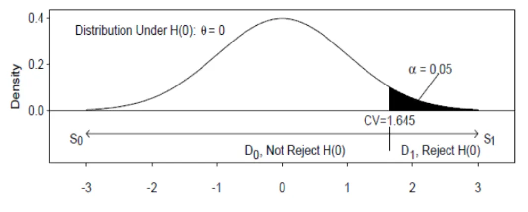
Figure 1. Null Hypothesis Significance Testing illustrated
Source:Gill (1999)10
We know that the area under the curve equates to 1 and can be represented by a probability density function. As we standardize the variable to a standard normal, we have a mean of zero and the spread is described by the standard deviation. Importantly, given that this curve’s standard deviation equals 1, we know that 68.26% of all observations are between -1 and +1 standard deviation, 95.44% of all observations will fall between -2 and +2 standard deviation and 99.14% of all cases are between -3 and +3 standard deviation. The shaded area represents the probability of observing a result from a sample as extreme as we observed, assuming the null hypothesis in population is true. For example, in a re-gression of Y on X the first step is to state the competing hypotheses:
Ho: bx = 0 Ha: bx ≠ 0
Where represents the observed value, μ0 represents the value under the null, represents the variance of the distribution and n represents the sample size (number of ob-servations). When the difference between the observed value and the value under the null increases, all other things constant, higher is the Z. Similarly, when the sample size gets bigger, all other things constant, the variance is lower and the Z is higher. The Z score is higher, and the p value statistic is lower. Therefore, the p value depends not only upon the effect magnitude but is, by definition, determined by the sample size.
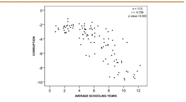
To make the estimation of the p value statistic more practical to political science scholars, we use observational data from the Quality of Government Institute11. The first step is to state both the null hypothesis and the alternative hypothesis.
Ho: r≥0 Ha: r<0
Theoretically, we expect a negative correlation between schooling years and corrup-tion (r< 0). Alternatively, the Ho (null hypothesis) states that the correlation between schooling years and corruption will be higher or equal to zero (r≥0). The p value statistic will inform the probability that the observed value is due to chance, assuming that the null hypothesis is true. We know from basic statistics classes the rule that “when the p value is low, the null hypothesis must go”. In other words, the lower the p value, the higher our confidence in rejecting the null hypothesis in favor of the alternative hypothesis. Figure 2 summarizes our empirical results.
The results suggest a strong negative (-0.799) correlation between average schooling years and corruption. The relationship is statistically significant (p value<0,000) with a sample of 113 country-cases. Following the 0.05 criteria, we should reject the null hypothe-sis of no or positive association between the variables. Then, we should conclude that there is a negative relationship between average schooling years and the level of corruption.
Most statistics handbooks present a rule of thumb of 0.1, 0.05 and 0.01 significance levels. It is important to stress that these are highly arbitrary cutoffs, and that the scholar should choose between them, preferably before analyzing the data. Fisher (1923) argues that:
If one in twenty does not seem high enough, we may, if we prefer it, draw the line at one in fifty (2 per cent point), or one in one hundred (the 1 per cent point). Personally, the writer prefers to set a low standard of significance at the 5 per cent point, and ignore entirely all results which fail to reach this level. A sci-entific fact should be regarded as experimentally established only if a properly de-signed experiment rarely fails to give this level of significance (Fisher, 1923: 85).
Through analyzing the relationship between schooling years and corruption, we es-tablished a 0.05 cutoff. Our p value is less than 0.000. To be sure, the p value is never exactly zero, but it is usual to report only three digits, therefore we interpret it as less than 0.01. So, given the null hypothesis that the correlation between schooling years and cor-ruption is higher or equal to zero, the p value of less than 0.000 means that the probability of finding a correlation as extreme as -0.799 is less than 0.000. Therefore we should reject the null hypothesis in favor of the alternative hypothesis.
After defining what the p value means, it is important to stress what is does not. It does not mean that the likelihood that the observed results are due to chance is less than 1%. Similarly, a p value of .01 does not mean that there is a 99% chance that your results are true, and a p value of .01 does not mean that there is a 1% chance that the null hy-pothesis is true. Additionally, you cannot interpret it as 99% evidence that the alternative hypothesis is true12. Lets follow Fisher’s classic definition: the p value is the probability, under the assumption of no effect (the null hypothesis H0), of obtaining a result equal to or more extreme than what was actually observed (Fisher, 1925).
Four Warnings on Signiicance Testing
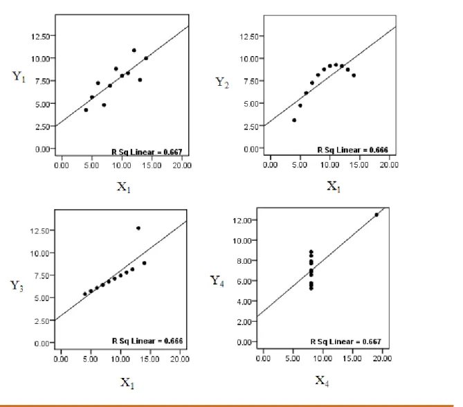
Anscombe (1973) demonstrated the importance of exploring data graphically before drawing inferences from it. He showed that different relationships between X and Y can be
summarized by the same statistics (F, standard error, b, beta etc). Figure 3 replicates his data, presenting four different relationships between variables with the same significant
p value.
Figure 3. Replication of Anscombe’s (1973) data
All graphs in Figure 3 gave the same p value statistic of 0.002. However, the graph-ical analysis shows that the nature of the relationship between the variables is markedly
different. For example, the upper-right graph shows a non-linear relationship. As long the scholar only examines the p value he would never get this information. Therefore, if
arguing that the relationship found using sample data could be generalized to the popula-tion. In addition, the researcher may fail to reject the null hypothesis after finding signifi-cant coefficient estimates, but this could be due an outlier effect (for example the bottom right graph in Figure 3). Basic statistics handbooks teach us that outliers can influence the probability of making Type I and Type II errors13. Thus, our first warning is that before interpreting the p value statistic, scholars must graphically analyze their data. To make our case more explicitly, we examine the correlation between the Human Development Index (HDI) and corruption.
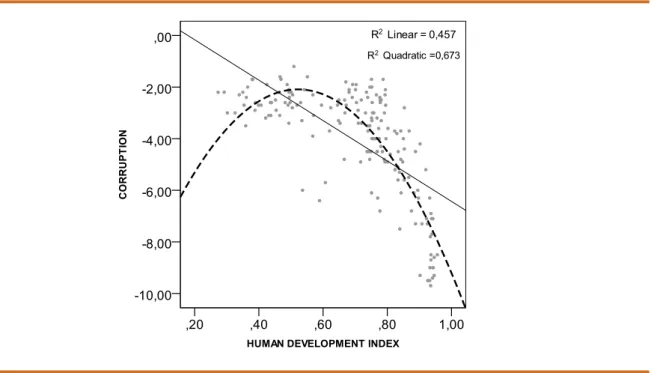
Figure 4. Correlation between Human Development Index and Corruption
In both cases the correlation is statistically significant (p value<0.000). However, when the researcher examines only the p value he would fail to acknowledge that the relationship between the variables is best described by a quadratic function (r2 =0.673) rather than by a linear function (r2 =0.457). The practical consequence of functional form misspecification 14in this case is the underestimation of the magnitude of relationship between the variables. Functional form misspecification can also lead to Type I and Type II errors.
To summarize, the careful graphical depiction of data is an essential step in empirical research. Scholars must avoid interpreting the p value statistic without graphically analyz-ing their data first. Breakanalyz-ing this important rule can lead to incorrect conclusions about political phenomena.
size n consists of n individuals from the population chosen in such a way that every set of n individuals has an equal chance to be the sample actually selected”. There are different sampling methods, considering the complexity of the population and the representative-ness of different characteristics. However, regardless of the method, if the sample is not random, the underlying assumptions of both the normal distribution and central limit the-orem16do not hold. Thus, sample statistics are no longer unbiased and efficient estimates of population parameters17. According to Smith (1983: 394), “the arguments for random-ization are twofold. The first, and most important for science, is that randomrandom-ization elimi-nates personal choice and hence elimielimi-nates the possibility of subjective selection bias. The second is that the randomization distribution provides a basis for statistical inference”.
Henkel (1976: 23) argues that “the manner in which we select samples from our populations is critical to significance testing, since the sampling procedure determines the manner in which chance factors affect the statistic(s) we are concerned with, and consequently affect the sampling distribution of the statistic”18. If the sample is random, the data is subject to the laws of probability and the behavior of estimated statistics as de-scribed by the sampling distribution. According to Moore and McCabe (2006), when you use systematic random samples to collect your data, the values of the estimated statistic neither consistently overestimate nor consistently underestimate the value of the popula-tion parameters.
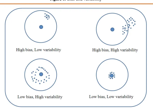
While randomization minimizes bias, the larger sample size reduces variability; the researcher is interested in producing estimates that are both unbiased and efficient (low variability) (see bottom right example).
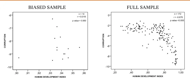
To make this claim more practical, we intentionally selected a biased sample and then we estimated the relationship between Human Development Index (HDI) and corrup-tion19. Figure 6 summarizes this information.
Figure 6. Correlation between Human Development Index and Corruption
BIASED SAMPLE FULL SAMPLE
Figure 7. Correlation between Human Development Index and corruption (random sample)
When dealing with a random sample of the same size (n=14), we observe a negative (-0.760) and statistically significant (p value = 0.002) correlation between the variables. In this case, when working with the random sample the scholar would reach the same conclusion based on population data.
Another potential problem is the use of a biased sample to reject the null hypothesis when it should not be rejected (type I error). Figure 8 illustrates this problem.
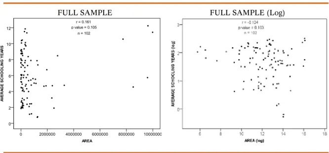
Figure 8. Correlation between Area and Average schooling years
FULL SAMPLE FULL SAMPLE (Log)
(logarithmic). In both cases, the correlation is not statistically significant. In other words, we cannot reject the null hypothesis that the estimated coefficient is equal to zero. So, we should conclude that geographical area and education are statistically independent. The following figure replicates this correlation with an income biased sample.
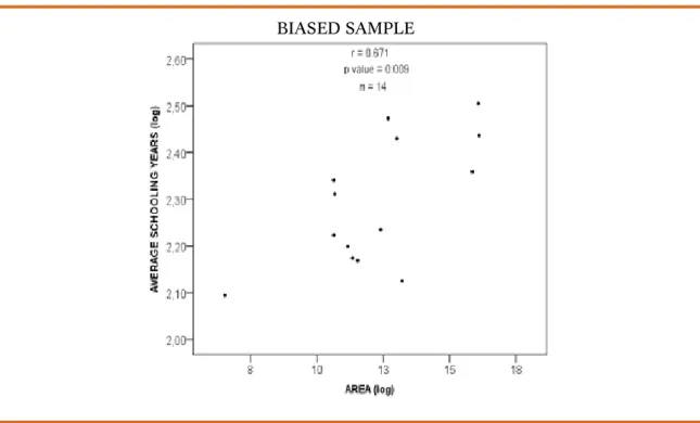
Figure 8a. Correlation between Area and Average schooling years
BIASED SAMPLE
The result is markedly different. When dealing with the income biased sample (n=14), we observe a positive (0.671) and statistically significant (p value = 0.009) correlation between the variables. In this case, we would wrongly reject the null hypothesis (type I error). Therefore, we would conclude that geographical area and schooling years are pos-itively associated.
Regardless of the sampling method design, we should meet the assumption of equiprobability, i.e. that each element in the population has the same chance of being selected. Non probabilistic samples cannot be used to make reliable statistical inferences. Therefore, we argue that it is pointless to interpret the p value of non-random samples.
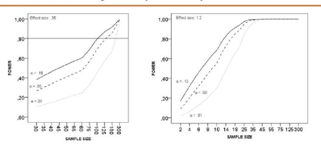
(1) Researchers should always design the study to achieve a power level of .80 at the desired significance level;
(2) More severe significance levels require larger samples to achieve the desired pow-er level;
(3) Conversely, power can be increased by choosing a less severe alpha. 4. Smaller effects sizes always require large sample sizes to achieve the desired power, and 5. Any increase in power is most likely achieved by increasing sample size.
To make our case, we partially replicate the experiment developed by The Institute for Digital Research and Education from the University of California21. We want to compare the means of two groups on a standardized mathematic test. Computationally, we used the Stata program function fpower to do the power analysis22. To do so, we had to define (1) the number of groups, (2) the effect size (delta)23and (3) the alpha level. We compared two groups with two different effect sizes (0.35 and 1.2), and we varied the alpha level in the three traditional cutoffs (0.1; 0.05 and 0.01). Figure 9 summarizes this information.
Figure 9. Test power and sample size
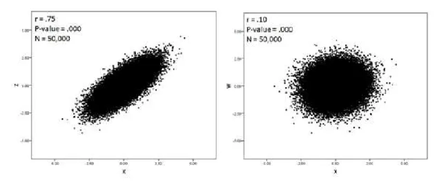
Figure 10. Different relationships, the same p value
According to Hair et al., (2006: 11), “by increasing sample size, smaller and smaller effects will be found to be statistically significant, until at very large samples sizes almost any effect is significant”. What is the meaning of a minute difference that is statistically significant? The relationship between X and W is statistically significant (p-value<0,000) but there is no substantive meaning on it. As stated by Gill (1999: 658), “political scien-tists are more interested in the relative magnitude of effects (…) and making only binary decisions about the existence of an effect is not particularly important”. Similarly, Luskin, (1991: 1044) points out that “to know that a parameter is almost certainly nonzero is to know very little. We care much more about its magnitude. But on this score the numbers do not speak for themselves”. Rather than focusing only on the p value, scholars should be looking at the magnitude of their estimates, the difference between group means, etc. The main conclusion is that when the sample is large enough (n>300), even marginal effects/ differences tend to be statistically significant. Scholars should be aware of this fact before claiming too much about their empirical findings.
In summary, whether we maintain the effect size constant and vary the sample size (figure 9), and whether we hold the number of cases constant and vary the magnitude of the observed relationship between the variables (figure 10), these procedures have a great effect on the size of the p value statistic. In either case, scholars should be cautions before extracting too much information from it, at the risk to reach wrong substantive conclusions.
entire population makes statistical inference unnecessary, because any differences or re-lationship, however small, is true and does exist” (Hair et al. (2006: 09). Introductory statistics handbooks teach us that we should use samples because they are faster and cheaper. If they are properly collected, they are also reliable. Keeping in mind that the role of inferential statistics is to draw inferences about the population from sample data, if the population is contained in all observations, estimation24is not needed. There is no reason to test the hypothesis since you already know your parameters.
Figure 11. Population, sample and statistical inference
In our view, if the sample size is equal to the size of the population, we cannot expect any error in estimating the true population parameter. Imagine a census of the population where men are shown to have an average income of X and women an average income of X+1. The mean difference between the groups is just one unit. As long we have informa-tion about all cases (the populainforma-tion), there is no room for estimating the expected value of the population parameter, since we already know it. The important issue is the magnitude of the difference, which is in this case very small. Our general position is that scholars should focus on the size of the expected effects, instead of worrying about the significance of the difference, especially in the situations we have defined here.
significance, 95% intervals, and all the rest, and just come to a more fundamental ac-ceptance of uncertainty” (Gelman, 2012a, n.p.). Regarding the sample-population debate, Bayesian scholars also tend to believe that we should always consider the population as a sample produced by an underlying generative process. The rationale is the following; the population you examined can be seen as a result of a more complex and dynamic process that can always generate a different population in some other moment in time. However, if you ask the same question to a frequentist researcher, he will likely answer that there is no meaning in the interpretation of the p value when the sample equals the population, since we already know the true parameter value.
As long as our main purpose is to introduce the logic of the p value statistic and is based on the frequentist position, we do not examine this debate more deeply. We encour-age readers to follow the references to obtain more information about this issue. Addition-ally, we advise students to adopt the following guidelines; (1) define your own position on the role of the p value statistic when the sample size equals the population; (2) once you pick one, you should be consistent with it, and (3) regardless of your technical position, you should always report not only the p value but also all the estimates in order to facil-itate other people’s assessment of your work. As a rule, you should always report all the information since your reader may not share the same opinions as you.
Conclusion
And if my estimated coefficient is not statistically significant? God help you! Unfor-tunately, many scholars still share this opinion. The evidence of this claim can be found in publication bias phenomena in various fields of knowledge. Gill (1999: 669) argues that “from the current presentation of null hypothesis significance testing in published work it is very easy to confuse statistical significance with theoretical or substantive importance”. In other words, political science students should be aware of the difference between statis-tical significance and pracstatis-tical significance. The p value cannot inform us about the magni-tude of the effect of X on Y. Similarly, the p value cannot help us to choose which variable explains the most. The p value cannot be compared across samples of different sizes. The p value cannot, by itself, answer the questions scholars are interested in. As noted by Moore and McCabe (2006), critical thinking about the use of significance tests is a sign of statis-tical maturity, however, scholars cannot make this decision when they do not fully under-stand the role of significance tests. Through this essay, we hope to help political science students make sense of the appropriate role of the p value statistic in empirical research.
References
ANSCOMBE, F. J. (1973), Graphs in Statistical Analysis, The American Statistician, vol. 27, nº 1, pp. 17-21.
BARRO, Robert J., and LEE, Jong-Wha. (2000), International Data on Educational Attainment: Updates and Implications, Center for International Development (CID) -Working Paper nº 42, Harvard University, <http://www.hks.harvard.edu/centers/cid/publications/faculty-working-papers/cid-working-paper-no.-42>.
BEGG, Collin B. and BERLIN, Jesse A. (1988), Publication Bias: A Problem in Interpreting Medical Data, Journal of the Royal Statistical Society – Series A, vol. 151, nº 3, pp. 419-463.
CARVER, Ronald P. (1978), The case against statistical significance testing, Harvard Educational Review, vol. 48, nº 3, pp. 378-399.
CARVER, Ronald P. (1993), The Case Against Statistical Significance Testing, Revisited, The Journal of Experimental Education, vol. 61, nº4, pp. 287-292.
COHEN, Jacob. (1988), Statistical Power Analysis for the Behavioral Sciences – 2nd Edition. Mahwah, NJ: Lawrence Erlbaum Associates.
COURSOUL, Allan and WAGNER, Edwin E. (1986), Effect of Positive Findings on Submission and Acceptance Rates: A Note on Meta-Analysis Bias, Professional Psychology, vol. 17, nº 2, pp. 136-137.
CRAMER, Duncan and HOWITT, Dennis L. (2004), The SAGE Dictionary of Statistics: A Practical Resource for Students in the Social Sciences. SAGE Publications Ltd., London.
DANIEL, Larry G. (1998), Statistical significance testing: A historical overview of misuse and misinterpretation with implications for the editorial policies of educational journals, Research in the Schools, vol. 5, nº 2, pp. 23-32.
DAVIDSON, Julia. (2006), Non-probability (non-random) sampling. The Sage Dictonary of Social Research Methods, <http://srmo.sagepub.com/view/the-sage-dictionary-of-social-research-methods/n130.xml>.
DE LONG, J. Bradford and LANG, Kevin. (1992), Are All Economic Hypotheses False? Journal of Political Economy, vol. 100, nº 6, pp. 1257-1272.
EVERITT, Brian S. (2006), The Cambridge Dictionary of Statistics – 3rd edition. New York: Cambridge University Press.
EVERITT, Brian S. and SKRONDAL, Anders (2010), The Cambridge Dictionary of Statistics.
New York: Cambridge University Press.
FISHER, Ronald A. (1923), Statistical Tests of Agreement Between Observation and Hipothesys,
Economica, nº 8, pp. 139-147.
GELMAN, Andrew, CARLIN, John B., STERN, Hal S. and RUBIN, Donald B. (2003), Bayesian Data Analysis – 2nd edition. New York: Chapman and Hall/CRC Texts in Statistical Science.
GELMAN, Andrew and STERN, Hal. (2006), The Difference Between “Significant” and “Not Significant” is not Itself Statistically Significant, The American Statistician, vol. 60, nº 4, pp. 328-331.
GELMAN, Andrew (2007), Bayesian statistics. Basel Statistical Society, Switzerland.
GELMAN, Andrew and WEAKLIEM, David. (2009), Of Beauty, Sex and Power, American Scientist, vol.97, pp. 310-317.
GELMAN, Andrew. (2012a), The inevitable problems with statistical significance and 95% intervals, Statistical Modeling, Causal Inference, and Social Science, < http://andrewgelman. com/2012/02/02/the-inevitable-problems-with-statistical-significance-and-95-intervals/>.
GELMAN, Andrew. (2012b), What do statistical p-values mean when the sample = the population?,
Statistical Modeling, Causal Inference, and Social Science, <http://andrewgelman.
com/2012/09/what-do-statistical-p-values-mean-when-the-sample-the-population/>.
GERBER, Alan, GREEN, Donald P. and NICKERSON, David. (2001), Testing for Publication Bias in Political Science, Political Analysis, vol. 9, nº 4, pp. 385-392.
GILL, Jeff. (1999), The Insignificance of Null Hypothesis Significance Testing, Political Research Quarterly, vol. 52, nº 3, pp. 647-674.
______ (2007), Bayesian Methods: A Social and Behavioral Sciences Approach – 2nd edition. New York: Chapman and Hall/CRC Statistics in the Social and Behavioral Sciences.
GREENWALD, Anthony G. (1975), Consequences of Prejudice Against the Null Hypothesis,
Psychological Bulletin, vol. 82, nº 1, pp. 1-12.
HAIR, Joseph F., BLACK, William C., BABIN, Barry J., ANDERSON, Rohph E. and TATHAM, Ronald L. (2006), Multivariate Data Analysis – 6ª edition. Upper Saddle River, NJ: Pearson Prentice Hall.
HENKEL, Ramon E. (1976), Tests of significance. Newbury Park, CA: Sage.
HUBERTY, Carl J. (1993), Historical origins of statistical testing practices: The treatment of Fisher versus Neyman-Pearson views in textbooks, The Journal of Experimental Education, vol. 61, nº4, pp. 317-333.
JORDAN, Michael I. (2009), Bayesian or Frequentist, Which are You?, Department of Electrical Engineering and Computer Sciences, University of California - Berkeley, Videolectures.net, <http://videolectures.net/mlss09uk_jordan_bfway/>.
KING, Gary, KEOHANE, Robert and VERBA, Sidney. (1994), Designing Social Inquiry: Scientific Inference in Qualitative Research. Princeton. N.J.: Princeton University Press.
LUSKIN, Robert C. (1991), Abusus Non Tollit Usum: Standardized Coefficients, Correlations, and R2s, American Journal of Political Science, vol. 35, nº 4, pp. 1032-1046.
McLEAN, James E., and ERNEST, James M. (1998), The Role of Statistical Significance Testing in Educational Research, Research in the Schools, vol. 5, nº 2, pp. 15-22.
MOORE, David S. and McCABE, George P. (2006), Introduction to the Practice of Statistics – 5th edition. New York: Freeman.
ROGERS, Tom (n.d), Type I and Type II Errors – Making Mistakes in the Justice System, Amazing Applications of Probability and Statistics, <http://www.intuitor.com/statistics/T1T2Errors. html>.
SAWILOWSKY, Shlomo. (2003), Deconstructing Arguments From The Case Against Hypothesis Testing, Journal of Modern Applied Statistical Methods, vol. 2, nº 2, pp. 467-474.
SCARGLE, Jeffrey D. (2000), Publication Bias: The “File-Drawer Problem” in Scientific Inference,
The Journal of Scientific Exploration, vol. 14, nº 1, pp. 91-106.
SIGELMAN, Lee. (1999), Publication Bias Reconsidered, Political Analysis, vol. 8, nº 2, pp. 201-210.
SIMES, John R. (1986), Publication Bias: The Case for an International Registry of Clinical Trials,
Journal of Clinical Oncology, vol. 4, nº 10, pp. 1529-1541.
SHAVER, J. (1992), What significance testing is, and what it isn’t. Paper presented at the Annual Meeting of the American Educational Research Association, San Francisco, CA.
SMITH, T. M. F. (1983), On the validity of inferences from Non-random Samples, Journal of the Royal Statistical Society – Series A (General), vol. 146, nº 4, pp. 394–403.
THE COCHRANE COLLABORATION. (n.d), What is publication bias? The Cochrane Collaboration open learning material, <http://www.cochrane-net.org/openlearning/html/ mod15-2.htm>.
VAN EVERA, Stephen. (1997), Guide to Methods for Students of Political Science. Ithaca, NY: Cornell University Press.
YOUTUBE. (2010), What the p-value?, <http://www.youtube.com/watch?v=ax0tDcFkPic& feature=related>.
APPENDIX 1
Table 01. Variable Description
Name Description Source QOG Code
Corruption CPI Score relates to perceptions of the degree of corrup-tion as seen by business people, risk analysts and the general public and ranges between 10 (highly clean) and 0 (highly corrupt). The index was inverted so that greater values equal more corruption.
www.transparency.org ti_cpi
Average School-ing Years
Average schooling years in the total population aged 25 and over.
www.cid.harvard.edu/ ciddata.ciddata.html (Barro and Lee, 2000)
bl_asyt25
HDI Composite index that measures the average achieve-ments in a country in three basic dimensions of human development: a long and healthy life, as measured by life expectancy at birth; knowledge, as measured by the adult literacy rate and the combined gross enrolment ratio for primary, secondary and tertiary schools, and a decent standard of living, as measured by GDP per capita in purchasing power parity (PPP) US dollars.
www.hdr.undp.org (UNDP, 2004)
undp_hdi
Area A country’s total area, excluding area under inland water bodies, national claims to continental shelf, and exclusive economic zones. In most cases the definition of inland water bodies includes major rivers and lakes.
Food and Agriculture Organization.
wdi_area
Source: Quality of Government Institute (2011).
Table 02. Descriptive Statistics
Label N min max mean standard deviation
Corruption 181 1.20 9.70 4 2.07
Average schooling years 103 0.76 12.25 6.02 2.90
Human Development Index 175 0.27 0.96 0.70 0.18
Area 190 2 17.098.240 702,337.27 1,937,230.60
Figure 13. Variable Histogram (log)
Notes
debate, since it falls outside of the context of this paper. For an online introduction to the frequentist-bayesian debate, see Jordan (2009). Readers interested in the Bayesian statistics should check Gelman, Carlin, Stern and Rubin (2003), Gill (2007) and Gelman (2007).
2 Publication biasrepresents the trend of both referees and scholars to overestimate the importance of statistical significant findings. According to Scargle (2000: 91), “publication bias arises whenever the probability that a study is published depends on the statistical significance of its results. This bias, often called the file-drawer effect because the unpublished results are imagined to be tucked away in researchers’ file cabinets, is a potentially severe impediment to combining the statistical results of studies collected from the literature”. Similarly, Everitt and Skrondal (2010: 346) define it as “the possible bias in published accounts of, for example, clinical trials, produced by editors of journals being more likely to accept a paper if a statistically significant effect has been demonstrated”. To get more information on publication bias see Greenwald (1975), Mahoney (1977), Coursoul and Wagner (1986), Simes (1986) and Begg and Berlin (1988), De Long and Lang (1992). In political science see Sigelman (1999) and Gerber, Green and Nickerson (2001). To see a simple definition see The cocharane Collaboration (n.d).
3 For a rebuttal of Carver arguments see Sawilowsky (2003).
4 Most data in political science comes from observational research designs rather than from experimental ones. For this reason, we use observational data to show the interpretation of the p value statistic when dealing with real political science research problems. As we know, observational data suffers from all sorts of shortcomings compared to experimental data. Scholars working with observational data face more challenges in making causal claims compared to those working with experiments. In addition, it is easier for a novice to understand examples based on observational data than from basic simulation.
5 A more systematic way of examining the role of the p value statistic in Brazilian political science literature is to survey all empirical papers and analyze how scholars have been interpreting the statistical significance of their empirical findings. The downside of this approach is the potential personal damage of exposing eventual mistakes. To minimize conflict, we prefer to focus on a more pedagogical approach.
6 Everitt (2006: 306) defines population as “any finite or infinite collection of ‘units’, which are often people but may be, for example, institutions, events, etc. Similarly, he defines sample as “a selected subset of a population chosen by some process usually with the objective of investigating particular properties of the parent population”.
7 According to Gill (1999: 648), “the current, nearly omnipresent, approach to hypothesis testing in all of the social sciences is a synthesis of the Fisher test of significance and the Neyman-Pearson hypothesis test”. For a historical overview of statistical significance see Huberty (1993). For an introduction to the statistical significance debate see Carver (1978; 1993), Henkel (1976), Shaver (1992), Daniel (1998), Sawilowsky (2003), Gill (1999), Gelman and Stern (2006) and Gelman and Weakliem (2009).
8 Van Evera (1997: 09) defines a hypothesis as “A conjectured relationship between two phenomena. Like Laws, hypothesis can be of two types: causal (I surmise that A causes B) and noncausal (I surmise that A and B are caused by C; hence A and B are correlated but neither causes the other).”
10 Regarding figure 1, Gill (1999) argues that the test procedure assigns one of two decisions (D0, D1) to all possible values in the sample space of T, which correspond to supporting either Ho or H1 respectively. The p value (associated probability) is equal to the area in the tail (or tails) of the assumed distribution under Ho, which starts at the point designated by the placement of T on the horizontal axis and continues to infinity. If a predetermined a level has been specified, then Ho is rejected for p values less than a, otherwise the p value itself is reported. Thus decision D1 is made if the test statistic is sufficiently atypical given the distribution under the Ho (Gill, 1999).
11 The description of the variables, basic descriptive statistics and distributions are presented in the appendix.
12 Too see this example in a cartoon see Youtube (2010).
13 A Type I error is the rejection of a true null hypothesis. Simply put, it is the chance of the test showing statistical significance when it is not present (false positive). The Type II error is the probability of failing to reject the null hypothesis when you should reject it (false positive) (Hair et al., 2006: 10). A more intuitive way of thinking about type I and type II errors is the following: imagine a man in a courtroom. He is not guilty (Ho). If he is convicted, the jury mistakenly rejected a true null hypothesis (type I error). Contrary, if the man is guilty (Ho) and the jury let him free, it means that they failed to reject a false null hypothesis (type II error). More details about this example can be found at Rogers (n.d).
14 Everitt and Skrondal (2010: 280) define misspecification as “a term applied to describe assumed statistical models which are incorrect for one of a variety of reasons, for example using the wrong probability distribution, omitting important covariates, or using the wrong link function. Such errors can produce inconsistent or inefficient estimates of parameters”.
15 “a probability sample is a sample chosen by chance. We must know what samples are possible and what chance, or probability, each possible sample has (…) the use of chance to select the sample is the essential principle of statistical sampling” (Moore and McCabe, 2006: 250-251).
16 Draw a random sample of size n from any population with mean μ and standard deviation. When n is large, the sampling distribution of the sample mean is approximately normal. Then, all properties of normal distribution apply to drawing inferences about population using sample data. According to Moore and McCabe (2006: 398), “the central limit theorem allows us to use normal probability calculations to answer questions about sample means from many observations even when the population distribution is not normal”.
17 By unbiased we mean that the sampling distribution of the statistic is equal to the true value of the parameter we are interested in. By efficient we mean that the estimated statistic has the lowest variability of all unbiased estimates.
18 The probability distribution of a statistic calculated from a random sample of a particular size. For example, the sampling distribution of the arithmetic mean of samples of size n, taken from a normal distribution with mean μ and standard deviation , is a normal distribution also with mean but with standard deviation (Everitt, 2006: 350).
19 The biased sample is an intentional selection of the 20 countries with the highest Gross Domestic Product (GDP).
that does not give all the individuals in the population an equal chance of being selected. According to Davidson (2006: 15), “forms of sampling that do not adhere to probability methods. Probability methods choose samples using random selection and every member of the population has an equal chance of selection. Some types of nonrandom sampling still aim to achieve a degree of representativeness without using random methods. Several different techniques are associated with this approach, for example accidental or convenience sampling; snowball sampling; volunteer sampling; quota sampling, and theoretical sampling. Convenience samples are also known as accidental or opportunity samples. The problem with all of these types of samples is that there is no evidence that they are representative of the populations to which the researchers wish to generalize”. Simple Random Sampling: A simple random sample (SRS) of size n is produced by a scheme which ensures that each subgroup of the population of size n has an equal probability of being chosen as the sample. Stratified Random Sampling: Divide the population into “strata”. There can be any number of these. Then choose a simple random sample from each stratum. Combine those into the overall sample; this is a stratified random sample. (Example: Church A has 600 women and 400 men as members. One way to get a stratified random sample size of 30 is to take an SRS of 18 women from the 600 women and another SRS of 12 men from the 400 men.) Multi-Stage Sampling: Sometimes the population is too large and scattered for it to be practical to make a list of the entire population from which to draw an SRS. For instance, when a polling organization samples US voters, they do not do an SRS. Since voter lists are compiled by counties, they might first do a sample of the counties and then sample within the selected counties. This illustrates two stages. In some instances, they might use even more stages. At each stage, they might do a stratified random sample on sex, race, income level, or any other useful variable on which they could get information before sampling. See: http://www.ma.utexas.edu/users/parker/sampling/srs. htm. Since sampling procedures design is not the focus of this paper, we restrict ourselves to discussing the role of the p value statistic for probabilistic samples. To get more information about sampling see http://www.sagepub.com/upm-data/40803_5.pdf
21 The full description of the original simulation is available at http://www.ats.ucla.edu/stat/ stata/dae/fpower.htm
22 Power analysis is the name given to the process of determining the sample size for a research study. The technical definition of power is that it is the probability of detecting a “true” effect when it exists.
23 According to Everitt and Skrondal (2010: 148), “most commonly the difference between the control group and experimental group population means of a response variable divided by the assumed common population standard deviation. Estimated by the difference of the sample means in the two groups divided by a pooled estimate of the assumed common standard deviation”.